
 Open Access Article
 This Open Access Article is licensed under a Creative Commons Attribution-Non Commercial 3.0 Unported Licence
A flexible data-free framework for structure-based de novo drug design with reinforcement learning†
Hongyan
Du‡
a,
Dejun
Jiang‡
a,
Odin
Zhang
a,
Zhenxing
Wu
a,
Junbo
Gao
a,
Xujun
Zhang
a,
Xiaorui
Wang
bc,
Yafeng
Deng
b,
Yu
Kang
 a,
Dan
Li
a,
Peichen
Pan
*a,
Chang-Yu
Hsieh
*a and
Tingjun
Hou
*a
a,
Dan
Li
a,
Peichen
Pan
*a,
Chang-Yu
Hsieh
*a and
Tingjun
Hou
*a
aCollege of Pharmaceutical Sciences, Zhejiang University, Hangzhou 310058, Zhejiang, China. E-mail: panpeichen@zju.edu.cn; tingjunhou@zju.edu.cn; kimhsieh@zju.edu.cn
bHangzhou Carbonsilicon AI Technology Co., Ltd, Hangzhou 310018, Zhejiang, China
cDr. Neher's Biophysics Laboratory for Innovative Drug Discovery, State Key Laboratory of Quality Research in Chinese Medicine, Macau Institute for Applied Research in Medicine and Health, Macau University of Science and Technology, Macao, 999078, China
First published on 19th October 2023
Abstract
Contemporary structure-based molecular generative methods have demonstrated their potential to model the geometric and energetic complementarity between ligands and receptors, thereby facilitating the design of molecules with favorable binding affinity and target specificity. Despite the introduction of deep generative models for molecular generation, the atom-wise generation paradigm that partially contradicts chemical intuition limits the validity and synthetic accessibility of the generated molecules. Additionally, the dependence of deep learning models on large-scale structural data has hindered their adaptability across different targets. To overcome these challenges, we present a novel search-based framework, 3D-MCTS, for structure-based de novo drug design. Distinct from prevailing atom-centric methods, 3D-MCTS employs a fragment-based molecular editing strategy. The fragments decomposed from small-molecule drugs are recombined under predefined retrosynthetic rules, offering improved drug-likeness and synthesizability, overcoming the inherent limitations of atom-based approaches. Leveraging multi-threaded parallel simulations combined with a real-time energy constraint-based pruning strategy, 3D-MCTS achieves remarkable efficiency. At a fixed computational cost, it outperforms other state-of-the-art (SOTA) methods by producing molecules with enhanced binding affinity. Furthermore, its fragment-based approach ensures the generation of more dependable binding conformations, exhibiting a success rate 43.6% higher than that of other SOTAs. This advantage becomes even more pronounced when handling targets that significantly deviate from the training dataset. 3D-MCTS is capable of achieving thirty times more hits with high binding affinity than traditional virtual screening methods, which demonstrates the superior ability of 3D-MCTS to explore chemical space. Moreover, the flexibility of our framework makes it easy to incorporate domain knowledge during the process, thereby enabling the generation of molecules with desirable pharmacophores and enhanced binding affinity. The adaptability of 3D-MCTS is further showcased in metalloprotein applications, highlighting its potential across various drug design scenarios.
Introduction
The objective of drug discovery is to identify compounds that have desirable bioactivity, safety, pharmacokinetic properties, and clinical therapeutic effects.1–4 However, the portion of the chemical space occupied by drug-like molecules is substantially scarce compared to the whole chemical space.5–7 As a result, drug discovery is often associated with a long development cycle, massive investment and high risk.8,9 Computer-aided drug design (CADD) provides an efficient and cost-effective way to optimize the process of chemical space sampling.10 Virtual screening (VS) is a widely used CADD method to identify active compounds from chemical libraries11,12 through molecular docking or a quantitative measure of structural similarity to active molecules.13 Nevertheless, the effectiveness of VS is largely constrained by the limited chemical space of compound libraries. Conversely, de novo drug design is unshackled from reliance on pre-existing compound libraries, and is able to explore a more expansive chemical space that affords the creation of more structurally diverse compounds.14,15In recent years, deep generative models have emerged as a promising technique for de novo drug design. However, most molecular generation models represent molecules in one-dimensional (1D) SMILES strings7,16–18 or two-dimensional (2D) molecular graphs,19,20 and generate molecules in a ligand-based paradigm without regard for the three-dimensional (3D) structure of the target binding site. In drug design, the ‘lock and key’ model emphasizes the importance of structural complementarity between the ligand and receptor, like a key fitting into a lock.21 To ensure desired receptor–ligand binding affinity, the ligand must have a 3D conformation that can form both favorable shape and energetic complementarity with the receptor, which has a significant impact on the generalization ability of molecular generation models in sampling target-specific molecules.22
Efforts have been made to encode the 3D structure of the protein pocket as a feature vector for conditional generation in the ligand-based paradigm,23–26 which however is insufficient for modeling the explicit interaction and geometric matching between the ligand and receptor. Several methods manipulate molecular topological structures through 1D SMILES or 2D molecular graphs, utilizing docking tools to ascertain the binding poses and docking scores of the molecules.27–29 This approach guides the generative algorithm towards the acquisition of molecules with elevated binding affinity. A series of deep learning (DL)-based models have been developed to enhance model performance. For example, LiGAN30 utilized a 3D convolutional neural network (CNN) to encode the complex structure into an atomic density grid representation, and generated molecules through a conditional variational autoencoder. However, the lack of rotational equivariance in the CNN and the limited grid resolution used notably impair prediction accuracy, leading to unsatisfactory quality of the generated molecules. To address this, SE-3 equivariant graph neural networks (GNNs) have emerged as a more apt model framework for encoding the 3D structures of ligand–receptor complexes. Within this domain, some methods employ diffusion models to generate entire molecules,31–34 while others construct them in an autoregressive manner.35–40 These models rely on a large number of ligand–receptor complex structures as the training data (CrossDocked2020 (ref. 41) with 22![[thin space (1/6-em)]](https://www.rsc.org/images/entities/char_2009.gif) 584102 binding conformations generated by molecular docking). Unfortunately, for many biological systems, such as protein–protein systems, peptide–protein systems, and small molecule–nucleic acid systems, large training data is lacking, which poses a challenge for developing deep generative models with high reliability. Furthermore, to the best of our knowledge, the majority of DL-based models operate at the atomic scale on molecular structures, with only a few utilizing fragments as the foundational units for molecule construction.34 There are some traditional methods that have utilized fragment-based approaches for in-pocket molecular generation.42–46 Notably, OpenGrowth47 employs a drug library as a training dataset, guiding the generation of molecules with enhanced synthetic accessibility and pharmacokinetics. Additionally, it can accommodate multiple receptor structures, thereby considering the flexibility of the target protein. In the initial stage of scaffold discovery or the later stage of structure optimization, medicinal chemists usually modify the structures of candidate molecules with specific fragments or functional groups.48–50 Therefore, fragment-based generation more closely aligns with chemical intuition and the current practice of de novo design, and through carefully designed fragment libraries and recombination rules, molecules generated in such a manner will usually have better synthesizability.
584102 binding conformations generated by molecular docking). Unfortunately, for many biological systems, such as protein–protein systems, peptide–protein systems, and small molecule–nucleic acid systems, large training data is lacking, which poses a challenge for developing deep generative models with high reliability. Furthermore, to the best of our knowledge, the majority of DL-based models operate at the atomic scale on molecular structures, with only a few utilizing fragments as the foundational units for molecule construction.34 There are some traditional methods that have utilized fragment-based approaches for in-pocket molecular generation.42–46 Notably, OpenGrowth47 employs a drug library as a training dataset, guiding the generation of molecules with enhanced synthetic accessibility and pharmacokinetics. Additionally, it can accommodate multiple receptor structures, thereby considering the flexibility of the target protein. In the initial stage of scaffold discovery or the later stage of structure optimization, medicinal chemists usually modify the structures of candidate molecules with specific fragments or functional groups.48–50 Therefore, fragment-based generation more closely aligns with chemical intuition and the current practice of de novo design, and through carefully designed fragment libraries and recombination rules, molecules generated in such a manner will usually have better synthesizability.
The search-based molecular generation method represents another approach to address the challenges associated with the aforementioned approaches of de novo drug design. Monte Carlo tree search (MCTS), a type of search-based method, has been proposed to circumvent some limitations of deep generative models. The MCTS method does not rely on a vast training set of samples, making it more flexible to be adapted to different molecular generation tasks under the guidance of an appropriate reward function, such as the molecular docking score. Specifically, ChemTS,51 introduced by Yang et al., is the first framework that implements MCTS for de novo molecular design, where a pre-trained RNN generative model is employed as a simulator to generate 2D molecules with specific properties, such as optimized lipid–water partition coefficient and synthesizability. Furthermore, Tashiro et al.52 optimized the reward function of the method to facilitate the generation of molecules with high asymmetry factors or high transition dipole strengths. Meanwhile, Li et al.53 extended the application of MCTS to structure-based molecular generation by introducing a target-free 3D molecular generative model. However, all of these MCTS based methods generate molecules in an atom-by-atom manner.
Contrary to the methods discussed previously that employ atoms as the fundamental units for molecular modification, in this study, we designed 3D-MCTS (Fig. 1), a novel search-based framework, by utilizing a more intuitive fragment-based generation paradigm, which enhances the synthesizability and rationality of binding conformations at the source. Uniquely, we leveraged MCTS with a well-designed fragment library by decomposing small-molecule drugs under predefined retrosynthetic rules. To combat the combinatorial explosion problem, we introduced two innovative features into the algorithm, including multi-threaded parallel simulation and a real-time energy constraint-based pruning strategy. This allows for the efficient identification of target molecules with superior binding affinity at a fixed computational cost. The fragment-based generation design also simplifies the complexity of molecular conformation modeling, ensuring that the generated molecules possess more reliable local and global conformations. 3D-MCTS achieves a success rate of 79.7% in generating molecules with the binding poses predicted by molecular docking software, which significantly outperforms the success rates achieved by Pocket2Mol and GraphBP (55.5% and 0.5%, respectively). Within the confines of identical computational resources, 3D-MCTS emerges as a more potent tool, outperforming conventional virtual screening by identifying a greater number of high-affinity hits and offering a broader exploration of the chemical landscape. The flexibility of 3D-MCTS permits the integration of expert knowledge at any point during the search process, allowing for the generation of molecules that align with specific pharmacophoric features, which usually plays a significant role in reducing false-positive rates in VS and structure optimization. Unlike most pharmacophore-conditioned deep generative models, 3D-MCTS does not rely on large amounts of ligand–receptor complex structure data or pre-generated pharmacophore models as training data. This offers an effective solution for designing domain knowledge-enhanced molecules for novel targets. The results of the generation of molecules toward metalloproteins further indicate that 3D-MCTS is highly adaptable and thus can be conveniently utilized across diverse tasks.
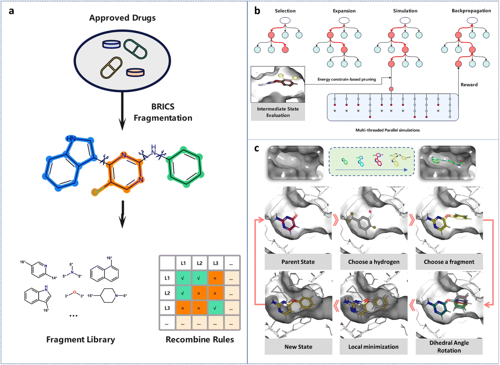 | ||
| Fig. 1 (a) The construction of the fragment library. Small molecule drugs in DrugBank were fragmentized by BRICS, and the highly frequent fragments were assembled into the fragment library. By labeling the connecting atoms of the fragments with isotopes, rules for fragment recombination were established, thereby ensuring the synthetic accessibility of the generated molecules. (b) The four steps for 3D-MCTS with the multi-threaded parallel simulations and real-time energy constraint-based pruning strategy. (c) The illustration of how a molecule is generated in the pocket fragment by fragment. | ||
Results and discussion
Binding affinities and drug-likeness of generated molecules on the test set
We assessed the effectiveness of 3D-MCTS in generating molecules by utilizing a commonly used test set derived from CrossDocked2020, and evaluated the quality of the generated molecules based on several metrics, including binding affinity (Vina score54), drug-likeness (QED55), synthetic accessibility, and molecular diversity. To compare 3D-MCTS with other deep learning (DL)-based generative methods, namely GraphBP35 and Pocket2Mol, we sampled 100 molecules per target in the test set. We set a threshold for the retaining molecules, T = Min(−8 kcal mol−1, original ligand score), where molecules were retained only if the binding affinities are less than the T value. The search process would terminate once 100 molecules were obtained. Additionally, we compared 3D-MCTS with three methods, AutoGrow4,27 Reinforced Genetic Algorithm (RGA)29 and MORLD,28 that employ a SMILES-based generation paradigm. AutoGrow4 and RGA employ genetic algorithms and molecular docking for de novo drug design, while MORLD combines reinforcement learning with molecular docking. RGA was developed based on AutoGrow4, introducing a network trained on the CrossDocked2020 dataset to guide the genetic algorithm's crossover and mutation to reduce its randomness.To ensure a fair comparison of the generation capabilities of different methods, we recorded the time taken to retain 100 molecules and compared the average Vina score and the best Vina score of the generated molecules (see Benchmark in Methods for details). For AutoGrow4, RGA and MORLD, we allowed them to iterate for the same amount of time as 3D-MCTS and recorded the binding affinities of the top 100 generated molecules. As presented in Table 1, the molecules generated by 3D-MCTS exhibited lower Vina scores, indicating improved energetic matching between the molecules and protein pockets. It took an average of 2232 seconds for 3D-MCTS to generate 100 molecules that meet the pre-defined requirements, which was comparable with the two DL-based methods, indicating its satisfactory generation efficiency. Of note, 3D-MCTS achieved superior results in generating molecules with improved binding affinity in 98% of the cases. In contrast, GraphBP and Pocket2Mol only achieved 50% and 60% success rates, respectively. We next evaluated the drug-likeness of the generated molecules, and the results revealed that 3D-MCTS could generate molecules with better drug-like profiles and higher binding affinities than the other methods. In order to address the concern of the synthetic accessibility of the generated molecules, we implemented the fragment recombination rules based on the Breaking of Retrosynthetically Interesting Chemical Substructures (BRICS) fragments during the design phase of 3D-MCTS. This approach largely confines the chemical space of the generated compounds to the regions that can be easily synthesized, and surprisingly maintains the molecular diversity at a level competitive to Pocket2Mol and AutoGrow4. For the three SMILES-based methods, while MORLD identified molecules with better binding affinity than AutoGrow4, it fell short in terms of drug-likeness, synthesizability, and structural diversity. Although AutoGrow4 generated molecules with slightly better structural diversity than 3D-MCTS, it lagged significantly behind in terms of binding affinity. The average performance of RGA was found to be inferior to that of AutoGrow4. This might arise from RGA's additional computational demands for training policy neural networks which is also mentioned in their paper. The results show that 3D-MCTS exhibits higher efficiency in exploring chemical space. This is due to the fact that 3D-MCTS grows molecules directly inside the pocket, which ensures real-time energy assessment. Thus, unreasonable energy states can be interrupted in a timely manner without the need to use molecular docking tools to systematically sample and score the conformations of each molecular state. It's worth noting that without the aid of docking tools, neither AutoGrow4 nor MORLD can provide the binding modes of the generated molecules, making them unsuitable for calculation of the ‘minimized score’ and ‘success rate’.
| Test set | GraphBP | Pocket2Mol | AutoGrow4 | RGA | MORLD | 3D-MCTS | |
|---|---|---|---|---|---|---|---|
| a Minimized score (kcal mol −1 ) represents the binding energy of ligands to protein pockets after GNINA minimization. The calculation is based on the binding poses from corresponding de novo design methods; docking score (kcal mol−1) represents the binding energy of ligands to protein pockets after Vina docking; Best and Average respectively represent the best score and average score among the 100 molecules sampled; QED is a quantitative measure of the drug-likeness of a molecule calculated by RDKit; SA is a score for the synthetic accessibility of a molecule calculated by RDKit. The score was normalized to the range (0, 1), with higher values indicating easier synthesis; Diversity is an indicator used to evaluate the structural diversity of the generated molecules (see the Methods section for details); For GraphBP and Pocket2Mol, Time represents the time required to generate 100 molecules (on a single NVIDIA Tesla V100 GPU); for 3D-MCTS, Time represents the time required to search for 100 molecules that meet the criteria (see the Results section for details); AutoGrow4, RGA and MORLD adopt the same iteration time as 3D-MCTS (on Intel(R) Xeon(R) Gold 6240R CPU @ 2.40 GHz); Success Rate is calculated on 100 targets in the test set. For a specific target, if the best minimized score of the generated molecules is better than that of the original ligands in the test set, the generation is considered successful on that target. | |||||||
| Best minimized score (↓) | — | −7.67 ± 1.5 | −8.90 ± 3.2 | — | — | — | −10.01 ± 1.2 |
| Average minimized score (↓) | −7.01 ± 2.31 | 7.62 ± 4.6 | −6.34 ± 2.3 | — | — | — | −8.55 ± 0.8 |
| Best docking score (↓) | — | −9.32 ± 1.5 | −9.42 ± 3.2 | −8.99 ± 1.4 | −8.50 ± 1.0 | −9.23 ± 1.2 | −10.32 ± 1.2 |
| Average docking score (↓) | −7.16 ± 2.12 | −1.26 ± 3.1 | −7.37 ± 2.4 | −7.18 ± 1.0 | −6.62 ± 0.5 | −7.67 ± 1.0 | −8.90 ± 0.7 |
| QED (↑) | 0.47 ± 0.2 | 0.50 ± 0.0 | 0.57 ± 0.1 | 0.63 ± 0.0 | 0.66 ± 0.0 | 0.38 ± 0.0 | 0.67 ± 0.1 |
| SA (↑) | 0.72 ± 0.1 | 0.52 ± 0.0 | 0.75 ± 0.1 | 0.53 ± 0.1 | 0.44 ± 0.0 | 0.24 ± 0.1 | 0.78 ± 0.1 |
| Diversity (↑) | — | 0.80 ± 0.0 | 0.69 ± 0.2 | 0.70 ± 0.0 | 0.90 ± 0.0 | 0.34 ± 0.1 | 0.62 ± 0.1 |
| Time (s) | — | 1059 ± 536 (V100 GPU) | 2503 ± 2207 (V100 GPU) | 2232 ± 2110 (24 CPU cores) | 2232 ± 2110 (24 CPU cores) | 2232 ± 2110 (24 CPU cores) | 2232 ± 2110 (24 CPU cores) |
| Success rate | — | 0.66 | 0.86 | — | — | — | 0.98 |
Quality of generated conformations
To evaluate the effectiveness of 3D-MCTS in modeling the plausibility of 3D molecular conformations, we assessed the rationality of the local conformations of the generated molecules and measured the difference between the bond angle distribution of the generated molecules and those of the ligands in the test set using the Jensen–Shannon divergence. Our results indicated that, in most cases, the bond angles of the molecules generated by 3D-MCTS were closest to those of the ligands in the test set (Table 2). We next sought to investigate whether the binding modes of the generated molecules within the pockets were plausible. A comprehensive evaluation work demonstrated that Vina can achieve a success rate of 72% in predicting the ligand binding poses when taking the top ten conformations for consideration. It should be eligible to use these poses as the “ground truth binding conformation” to estimate the quality of binding poses from generative methods.56 The minimum root-mean-square deviation (RMSD) between the conformation of the generated molecule and the ground truth binding conformation was then calculated to assess the plausibility of the conformations of the generated molecules. The results demonstrated that the molecules generated by 3D-MCTS exhibited the highest similarity to the binding modes produced by Vina docking (Fig. 2). When the threshold of RMSD was set to 2 Å, the success rate of 3D-MCTS in predicting the binding modes of the generated molecules was 79.7%, which surpassed those of Pocket2Mol and GraphBP (55.5% and 0.5%, respectively). Although the Vina score was used to guide the fragment growth, our model did not make use of the global docking function of Vina to manipulate molecular conformations, and relied instead on our designed protocol of fragment-by-fragment generation and energy optimization.| Bond angle | GraphBP | Pocket2Mol | 3D-MCTS |
|---|---|---|---|
| CCC | 0.42 | 0.06 | 0.07 |
| CCO | 0.49 | 0.16 | 0.16 |
| CNC | 0.37 | 0.13 | 0.07 |
| NCC | 0.36 | 0.15 | 0.05 |
CC ![[double bond, length as m-dash]](https://www.rsc.org/images/entities/char_e001.gif) O O |
0.36 | 0.34 | 0.18 |
| COC | 0.51 | 0.48 | 0.32 |
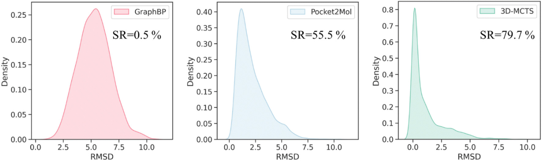 | ||
| Fig. 2 The RMSD distributions of the conformations generated by different methods. The RMSDs are calculated between the binding conformations of the molecules generated by the generative methods and the “ground truth binding conformations” predicted by Vina global docking. | ||
Comparison with the chemical space exploration capability of virtual screening
Virtual screening is another widely used computational technique in drug discovery to search libraries of small molecules in order to identify those structures most likely to bind to a drug target. One of the primary disadvantages of virtual screening is its high dependency on the compound library used. The quality, diversity, and size of the library can significantly influence the screening results.57,58 While a larger compound library in virtual screening may offer a greater diversity of active molecules, it also comes with the drawback of increased computational resource consumption.59 To address this concern, we conducted a comparison between our 3D-MCTS method and a Vina docking-based virtual screening approach, specifically focusing on their capabilities to explore active chemical space under equivalent computational resources (see the Methods section for details).To provide a fair comparison between virtual screening (VS) and 3D-MCTS, we established a binding affinity threshold for each target in the test set based on the results of virtual screening. Molecules scoring better than this threshold were designated as ‘potential hits’. We then counted the number of such hits obtained by both VS and 3D-MCTS under equivalent computational resources and assessed the structural diversity of these hits. Our results, as shown in Table 3, indicate that 3D-MCTS is capable of identifying a significantly larger number of ‘potential hits’ compared to traditional virtual screening methods. Furthermore, these hits exhibit a high degree of skeletal diversity. To visualize the chemical space explored by both methods, we plotted the distribution of the top 0.1% of hits obtained. Employing t-SNE for visualization, we found that 3D-MCTS explores a broader swath of chemical space, much of which remains unexplored by traditional virtual screening methods (Fig. 3b). These findings suggest that 3D-MCTS can transcend the inherent limitations of specific compound libraries, offering a more efficient and diverse exploration of chemical space. This yields a richer and more structurally diverse set of ‘potential hits’, thereby providing a more comprehensive selection pool for subsequent compound enrichment and bioactivity evaluation. It's important to highlight that the outcomes of virtual screening are influenced by various parameters, including the choice of docking tools, their settings, the selected compound libraries, and the pre-screening filtering criteria. Our comparison serves primarily as a proof of concept, demonstrating the superior capability of 3D-MCTS in navigating the chemical space over traditional virtual screening.
| Virtual screening | 3D-MCTS | Virtual screening | 3D-MCTS | |
|---|---|---|---|---|
| 0.1% | 1% | |||
| a Total Number of Molecules denotes the count of all molecules subjected to Vina docking in the case of virtual screening. For 3D-MCTS, this metric signifies the count of intermediate molecular states encountered throughout the search process. | ||||
| Threshold score (kcal mol−1) | −9.2 | −9.2 | −8.8 | −8.8 |
| Total number of molecules | 10000 |
20556 |
10000 |
20556 |
| Number of molecules that scored better than the threshold | 10 | 387 | 100 | 775 |
| Number of Murcko scaffolds | 10 | 314 | 98 | 647 |
| QED (↑) | 0.56 | 0.61 | 0.56 | 0.62 |
| SA (↑) | 0.82 | 0.78 | 0.82 | 0.78 |
 | ||
| Fig. 3 (a) Distribution of the number of molecules generated by 3D-MCTS that meets the 0.1% binding affinity threshold across 100 targets. (b) Chemical space distribution of potential hits explored by virtual screening and 3D-MCTS (visualized using t-SNE). | ||
Stable performance in the sparse data scenarios
Deep generative models have exhibited remarkable performances in image recognition60–62 and natural language processing,63–65 as well as some applications within the life science domain.4,66–69 However, it has been widely acknowledged that the effectiveness of DL-based models is highly dependent on the quality and quantity of training data. When the training set is small and does not align well with the expected test cases, DL models often suffer from a severe performance drop.70 In contrast, search-based molecular generation algorithms have the ability to produce stable and high-performing results without heavy reliance on training data. These algorithms can leverage mature reward functions to guide their search for optimal solutions. To confirm our hypothesis, we developed two test sets, namely high similarity and low similarity, composed of protein pockets that bear high (similarity > 0.6) and low similarity (similarity < 0.4) relative to those in the training set (see the Pocket similarity and clustering part in the Methods for details). As illustrated in Fig. 4a and 3b, 3D-MCTS generated molecules without significant differences in the binding affinities of the molecules generated for the two test sets, whereas Pocket2Mol displayed an obvious discrepancy in its modeling capability for the two test sets. This suggests that the protein pockets which can be well handled by Pocket2Mol are strongly confined to the in-distribution cases defined by the training data. When the pocket structures of the test targets substantially deviate from those of the training set, the DL-based model may experience difficulties in sampling ligand molecules that fit the pockets.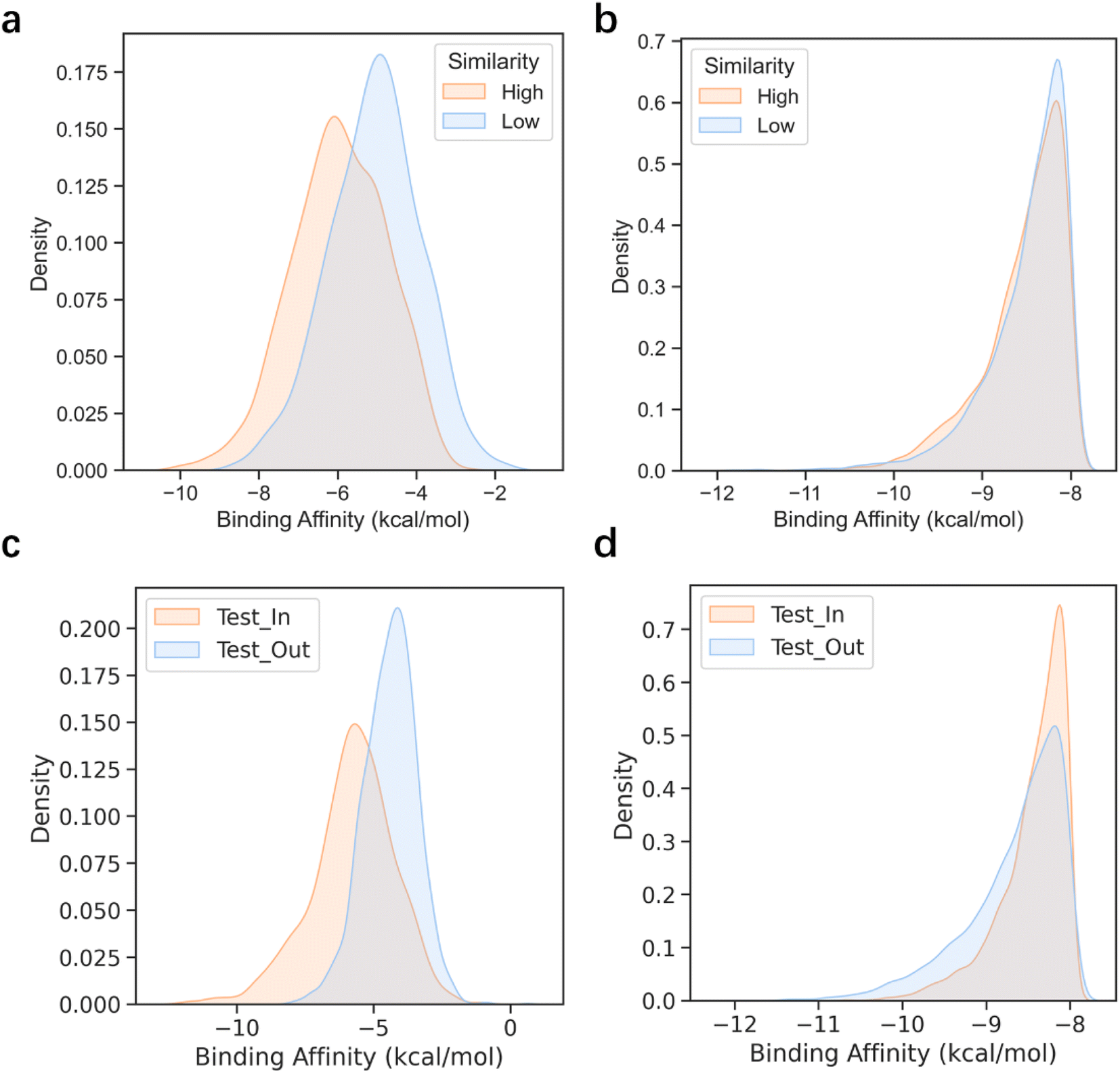 | ||
| Fig. 4 The binding affinity distribution of the generated molecules on different test sets. (a) The performance of Pocket2Mol on the test sets with high and low similarity with the training set, respectively. (b) The performance of 3D-MCTS on the test set with high and low similarity with the training set, respectively. (c) The performance of Pocket2Mol on the Test_In and Test_Out sets. (d) The performance of 3D-MCTS on the Test_In and Test_Out sets. | ||
To further validate our hypothesis, we clustered the CrossDocked2020 dataset based on the similarity of pockets and created the training set and test set according to the clustering results (see the Pocket similarity and clustering part in the Methods for details). Molecule samples were generated separately on the two test sets, Test_In and Test_Out, which included the pockets inside and outside the training set clusters, respectively. Similar conclusions were drawn for this experiment as well (Fig. 4c and d). Specifically, the molecules sampled for the Test_Out test set by Pocket2Mol showed inferior binding affinities to the target pockets than those generated by 3D-MCTS, which demonstrated a more stable performance of 3D-MCTS for different test sets. Thus, this result indicates that search-based 3D-MCTS possesses conspicuous advantages in targets with relatively sparse training data.
Flexibility of the search framework
The search-based method of 3D-MCTS holds an inherent advantage over data-driven DL models in terms of flexibility, which is achieved by not relying on any specific dataset. To accomplish a specific generation task, a data-driven DL model requires a training process to learn useful input–output relations from some data, and the trained model can only solve specific problems resembling those seen during the training. Modifications to the model architecture and retraining are usually necessary for different needs, such as a new therapeutic target or a change of preference over the desired physicochemical profile for an ideal molecule. In contrast, search-based methods enable us to more effectively adjust the search direction by manipulating the reward function and the preference of molecular state selection, facilitating the attainment of various molecular generation requirements in a flexible manner. We assessed the flexibility of the search algorithms in two scenarios: (1) introducing a new reward component based on the pharmacophore model to direct the search towards a chemical space guided by domain knowledge, and (2) utilizing the corresponding reward function to facilitate the molecular generation for specific systems (i.e., metalloprotein systems).| PDB | Ligand score (kcal mol−1) | Number of molecules (↑) | Average score (kcal mol−1, ↓) | QED (↑) | SA (↑) | |||||
|---|---|---|---|---|---|---|---|---|---|---|
| Test set | Baseline (Pocket2Mol) | Off | On | Off | On | Off | On | Off | On | |
| a Off represents the standard 3D-MCTS, which only considers binding affinity as the reward; On represents a version of 3D-MCTS that incorporates domain knowledge based on pharmacophores during the generation process. | ||||||||||
| 1fmc | −9.32 | −6.92 | 88 | 160 | −9.52 | −9.94 | 0.69 | 0.63 | 0.80 | 0.74 |
| 3g51 | −7.63 | −8.31 | 135 | 167 | −9.55 | −9.90 | 0.65 | 0.63 | 0.79 | 0.76 |
| 5q0k | −9.24 | −6.67 | 15 | 58 | −9.52 | −9.90 | 0.63 | 0.66 | 0.80 | 0.80 |
| 1phk | −8.14 | −10.72 | 433 | 737 | −9.52 | −10.09 | 0.65 | 0.66 | 0.76 | 0.75 |
| 4f1m | −6.58 | −6.78 | 18 | 46 | −9.29 | −9.78 | 0.70 | 0.58 | 0.79 | 0.79 |
| 1e8h | −8.83 | −8.72 | 264 | 353 | −9.55 | −10.08 | 0.70 | 0.65 | 0.78 | 0.77 |
| 1ai4 | −6.28 | −5.60 | 114 | 81 | −9.41 | −9.86 | 0.61 | 0.63 | 0.82 | 0.81 |
| 3w83 | −3.91 | −3.30 | 51 | 83 | −9.54 | −9.86 | 0.64 | 0.60 | 0.78 | 0.74 |
| 5d7n | −7.56 | −7.71 | 128 | 114 | −9.43 | −9.97 | 0.63 | 0.65 | 0.78 | 0.77 |
| 5aeh | −11.93 | −10.11 | 593 | 843 | −10.26 | −10.78 | 0.64 | 0.68 | 0.73 | 0.79 |
| 4qlk | −8.48 | −7.34 | 238 | 366 | −9.48 | −9.97 | 0.57 | 0.66 | 0.76 | 0.80 |
| 3hy9 | −8.12 | −6.66 | 528 | 768 | −9.51 | −10.06 | 0.64 | 0.65 | 0.79 | 0.80 |
| 4m7t | −7.81 | −8.24 | 525 | 701 | −9.69 | −10.07 | 0.65 | 0.64 | 0.76 | 0.78 |
| Average | −7.99 | −7.47 | 241 | 344 | −9.56 | −10.02 | 0.65 | 0.64 | 0.78 | 0.78 |
However, relying solely on the Vina score as a reward in the reinforcement learning method may not always produce satisfactory results, due to the insufficient accuracy of the scoring function. This problem is also common in DL-based generative models, which rely on the energy-based scoring function for constructing training datasets and evaluating the binding affinities of generated molecules. The introduction of prior knowledge may reduce the bias brought by the scoring function and guide the sampling towards a more valid domain. To verify this, we next tested the model for generating molecules targeting HMGR (3-hydroxy-3-methylglutaryl-coenzyme A reductase), which is a critical enzyme to catalyze the conversion of HMG-CoA (3-hydroxy-3-methylglutaryl-coenzyme A) to mevalonate. Given the central role of HMGR in cholesterol synthesis, it has been regarded as an essential target in drug discovery, particularly for treating CVD (cardiovascular disease).74 Elevated cholesterol levels, particularly LDL-C (low-density lipoprotein cholesterol), are a major risk factor for CVD. Statins are commonly used HMGR inhibitors due to efficient activity in lowering serum cholesterol levels.75 The binding modes of statins revealed they occupy part of the binding site of HMG-CoA, blocking its binding to HMGR, and commonly form conserved hydrogen bonds with amino acids such as Lys735, Arg590, and Lys691 near the binding site75 (Fig. 5a). To evaluate the accuracy of scoring functions on HMG-CoA, we scored the inhibitors and decoy molecules provided by DEKOIS2.0 using Vina and Glide SP. The areas under the receiver operating curves of the two scoring functions were 0.692 and 0.971, respectively (Fig. 5b), suggesting that the Glide SP score is a better option for this system and can be used as the proxy for the true quality of generated molecules. We further analyzed the predicted binding conformations of the active ligands and found that Glide SP could successfully reproduce the key interactions between the ligands and receptor. To evaluate the impact of introducing the prior knowledge based on the pharmacophore model on the search process, we used Glide SP as the evaluation criterion while keeping the Vina score as the reward. Our results showed that the incorporation of the prior knowledge improved the Glide SP scores of the generated molecules, indicating a greater likelihood of becoming active molecules (Fig. 5c). Moreover, the searched molecules with desirable Glide SP scores demonstrated similar binding modes with statins (Fig. 5d).
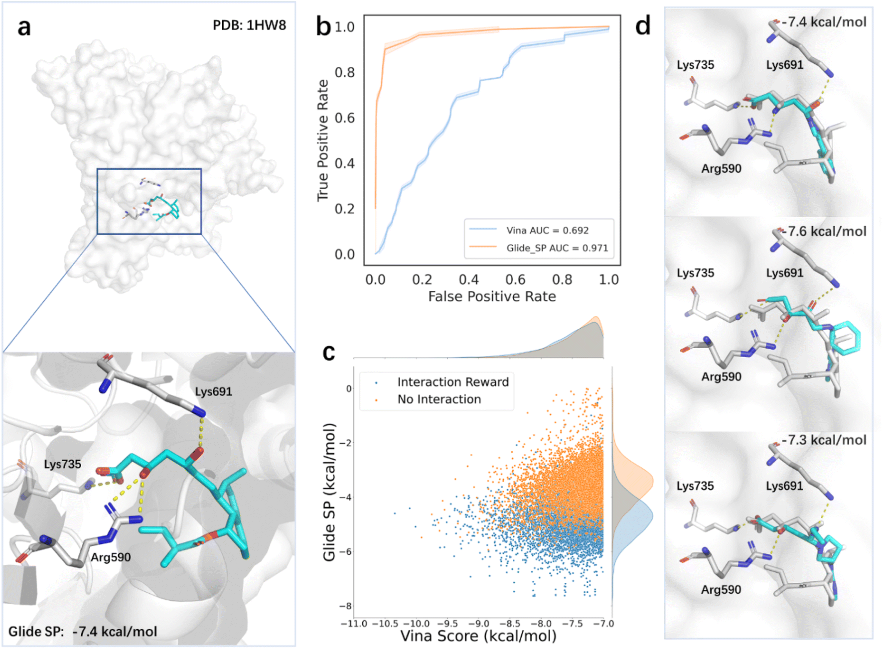 | ||
| Fig. 5 The influence of experts' prior knowledge on the search results for HMGR. (a) The binding mode of compactin with HMGR. The dashed lines in yellow indicate the hydrogen bond interactions between compactin and the binding site. (b) The receiver operating curves of Vina and Glide_SP to evaluate their virtual screening power on HMGR. (c) The score distribution of the molecules generated by the standard 3D-MCTS and expert prior knowledge-enhanced 3D-MCTS, respectively. (d) Examples of the generated molecules (shown as the cyan stick) that display the same binding mode with compactin (shown as the gray stick). | ||
| Protein | Ligand score (pIC50) | Best metal score | ||
|---|---|---|---|---|
| 3D-MCTS | 3D-MCTS + metal | Pocket2Mol | ||
| blaB1 | 6.31 | 6.81 | 8.90 | 7.08 |
| QCs | 7.02 | 6.53 | 8.21 | 6.06 |
| SusB | 6.90 | 6.94 | 8.23 | 7.13 |
Metal ions in metalloproteins typically form coordination bonds with amino acids and ligands in the binding sites, with the former providing empty orbitals and the latter providing lone electron pairs. Fig. 6 illustrates the distribution of the lone pairs of atoms (oxygen, nitrogen, or sulfur) in the molecules generated by the standard 3D-MCTS and 3D-MCTS enhanced by MetalProGNet. Our analysis revealed that the distribution of the lone pair donors of the former was relatively disordered, while the latter generated more lone pair donors near the metal atoms to form coordination bonds. This suggests that introducing a specific reward function in the search process can effectively regulate the arbitrariness in exploring chemical space and guide the generation of molecules that conform to the expected physical intuition. The testing on metalloproteins showcases the adaptability and versatility of 3D-MCTS. Researchers have developed scoring methods for various systems, including protein–peptide systems,79 covalent ligands80 and protein–protein interactions.81 However, the lack of large-scale training data could hamper the effectiveness of molecular generation methods based on deep generative models. With appropriate scoring functions, 3D-MCTS could efficiently and accurately perform oriented generation tasks in various application scenarios.
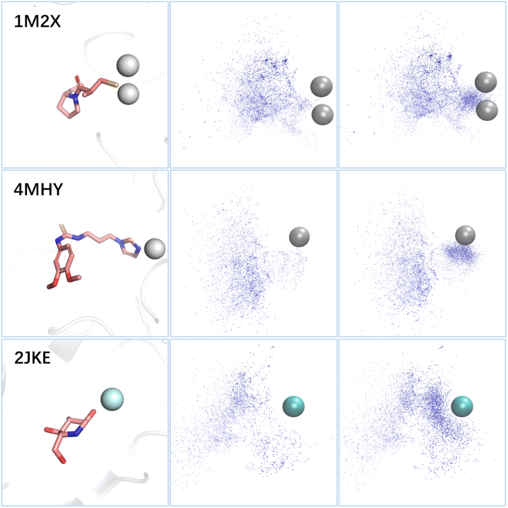 | ||
| Fig. 6 The influence of the metal-specific reward on the search results. (Left) The binding modes of ligands in three metalloproteins. The metal ions are represented in ball mode, wherein the zinc ion appears in gray and the calcium ion in cyan. (Middle) The distribution of the lone pair donors of the molecules generated by the standard 3D-MCTS. (Right) The distribution of the lone pair donors of the molecules generated by the MetalProGNet-enhanced 3D-MCTS. | ||
Conclusion
In this study, we present a unique structure-based de novo drug design method that employs MCTS in conjunction with an intricately designed fragment library. This innovative approach successfully circumvents the constraints inherent in the conventional atom-by-atom molecular generation paradigm. Our method uses fragments, derived from the disassembly of small molecule drugs through the BRICS method, as the building blocks. The use of these fragments bestows the generated molecules with the best intrinsic chemical synthesizability and drug-likeness compared with other methods. Additionally, this approach simplifies molecular conformation modeling and ensures the validity of the molecules' intermediate states. This enables an ongoing energy evaluation and optimization throughout the generation process. As a result, 3D-MCTS generates molecules with not only optimal local conformations but also a superior quality of molecular binding modes compared to existing SOTAs (with an improvement of 43.6% in success rate). To optimize the search efficiency, our algorithm incorporates multi-threaded parallel simulation and a real-time energy constraint-based pruning strategy. This allows it to identify target molecules with improved target binding affinities (−2.0 kcal mol−1 better than those of SOTAs) at a fixed computational cost. Under equivalent computational conditions, 3D-MCTS proves more effective than traditional virtual screening in discovering a larger set of high-affinity hits, underscoring its advanced capacity for chemical space exploration. Crucially, the performance of 3D-MCTS is independent of training data, which ensures its robust and stable molecule generation across different targets. This contrasts with DL-based SOTA methods, which underperform on targets exhibiting low similarity to their training sets. The flexibility of 3D-MCTS facilitates the integration of expert knowledge during the search process which allows for a dynamic adjustment of the molecular search direction and leads to the identification of more molecules that align with specific pharmacophoric features. As a proof of concept, by utilizing a specific reward function, we have extended our molecular generation approach to metalloproteins. This illustrates the high adaptability of 3D-MCTS and highlights its potential applicability across diverse task scenarios. We anticipate that 3D-MCTS will be used in a wide range of applications that require specific molecular recognition.Methods
Problem definition
We developed a general fragment-based molecular generation framework based on the MCTS algorithm to generate 3D molecules that match a specific protein pocket in terms of geometry and energy. Since the generated molecules depend on the previous state of the modified molecule, we mathematically model the process of fragment growth as a Markov decision process (MDP). The formal representation of MDP is M = (S, A, f, R), where S represents the state space. For the task of 3D molecular generation, the state of a molecule is determined by its topological structure and 3D conformation, which can be represented as S = Stop × Sconf_l × Sconf_g. Here, Stop denotes the topology space of the molecule, while Sconf_l and Sconf_g represent the local conformation space (determined by the bond length, bond angle, and dihedral angle within the molecule) and the global conformation space (determined by the relative spatial position of the molecule and the protein pocket), respectively.A denotes the action space (i.e., the way of modifying the molecule). Unlike previous studies that employ SMILES strings for 2D molecular generation, we manipulate both the topology and conformation of the molecule in the protein pocket during the action selection process. As our approach is based on fragment-wise generation, we manipulated the molecule in terms of fragments. Specifically, we performed three different actions to transform the molecule state from st to st+1. First, we determined the substitution position, where all heavy atoms connected to hydrogen atoms are treated as potential substitution positions to simplify the processing. Second, we selected a suitable fragment from the fragment library and attached it to the selected heavy atom from the previous step. We considered drug-likeness and synthesizability when building the fragment library. We used the BRICS82 rules to fragmentize the small-molecule drugs in the DrugBank database83 and counted the frequency of each fragment (Fig. 1a). We then selected the top 50 most frequently occurring fragments as the fragment library, considering their drug-likeness and synthetic accessibility. The BRICS method identifies and cleaves retro-synthetically relevant bonds in the molecule, marking the atoms with specific isotopes based on their chemical environment at the cut site. This method defines a set of rules for connecting atoms, ensuring the synthetic feasibility of the resulting molecules. We chose fragments that meet the criteria according to the recombination rules and connected them to the heavy atom selected in the previous step. Finally, we rotated the newly introduced rotatable bond at 15 degree intervals to generate multiple binding conformations and retained the ones with lower energies. By performing the three consecutive actions of selecting the substitution position, fragment connection, and conformation selection based on the energy advantage, we transformed the molecule state from st to st+1.
f:S × A → S denotes the state transition function. In the process of fragment linking, the state transition is deterministic, and thus, for any given state–action pair, p(st+1|st,at) = 1. That is to say, by performing a modification operation, the current molecule will certainly transition to the next state with the modified structure.
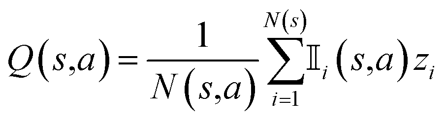
R represents the reward obtained under a given molecule state. Our objective is to choose an action that maximizes the expected reward. To achieve this goal, we can approximate the expected reward by repeating simulations using the following formula:84
 | (1) |
 is an indicator function that takes a value of 1 if action a is taken in the i-th round from state s, and 0 otherwise. Furthermore, zi represents the final reward obtained in the i-th round of simulation from state s. It should be noted that the larger the value of Q(s,a), the higher the expected reward of taking action a from state s.
Monte Carlo tree search
In a general tree-based search, every node and its descendants should be evaluated until the final solution is found. However, for tasks with exponentially increasing numbers of nodes, this brute-force search method proves to be inefficient. A prime example of such a task is the game of Go. Nevertheless, through MCTS, a machine has achieved top-level performance in Go by focusing on favorable descendant nodes and paying less attention to the others.85 This approach enables the exploration of a minimal number of nodes to obtain the optimal solution. MCTS employs a tree structure to simulate and evaluate the value of each action at every step, while utilizing previously estimated action values to guide the search process toward a higher reward.86 The basic MCTS process involves four steps per iteration: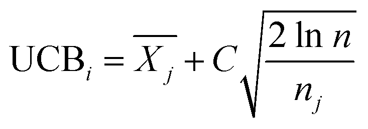 | (2) |
| Child = Roulette(UCB1, UCB2, …, UCBj, …, UCBn) | (3) |
 is the average reward of node j up to this point, nj is the number of times node j is selected, n is the total iteration number, and C is a parameter that balances exploration and exploitation. The first term,
  , is biased towards exploitation, selecting nodes that have better average performance. The second term,
  , is biased towards exploration, selecting nodes that are less visited. UCB strikes a balance between exploitation and exploration, enabling the search process to converge quickly while avoiding getting trapped in local optima. Prior to calculating the UCB value, we first normalize the average reward of all child nodes to (0, 1). To mitigate the risk of getting stuck in a local optimum, we do not select the node with the best UCB value directly but adopt a roulette wheel random selection policy instead.
(1) Atomic collision: a collision is deemed to have occurred when the distance between any non-bonded atoms in the system is less than the sum of their covalent radii.
(2) Unfavorable energy: if the introduction of a new fragment leads to an increase in the Vina score, the fragment is considered to have an unfavorable impact on the overall fit between the molecule and the pocket. To avoid local optima, we provide an energy buffer of 2 kcal mol−1, such that only when Score(st+1) − 2 kcal mol−1 > Score(st) is satisfied does st+1 meet the termination criteria.
(3) Drug-like properties: we observed that the drug-like properties of most molecules deteriorate as the molecule volume increases. Thus, employing QED as a termination criterion prevents the search algorithm from unreservedly increasing the molecule volume for a better Vina score.
(4) Molecular weight: when the molecular weight exceeds 500, st+1 meets the termination criteria.
Workflow of molecular generation
The search process of 3D-MCTS continuously builds a tree of molecular states, where each node represents a molecule to be modified, and we keep retaining molecules that meet certain criteria during the search process. The starting point for 3D-MCTS is a protein pocket and an initial fragment molecule with a determined binding pattern, which can be obtained from a crystal structure or predicted by a molecular docking tool (Fig. 1c). We designate this starting fragment as s0. Subsequently, we apply the BRICS rules to identify the types of heavy atoms at substitutable positions in s0, and mark them with isotopes. Next, we select suitable fragments from the fragment library and connect them to the identified positions based on the isotopes and fragment recombination rules. After that, we obtain multiple conformations of the molecule by rotating the newly introduced rotatable bonds. During the adjustment, only the positions of atoms in the new fragment change, while the atoms in s0 remain in their original positions. To obtain a more reasonable overall conformation of the molecule and consider the impact of the newly introduced fragment on the overall binding conformation, we perform energy minimization of the entire molecule using Gnina,87 resulting in a new molecular state, s1. This process is iterated to obtain s2, s3, …, st, st+1. Finally, the molecular states that meet the user's requirements are preserved in SDF format.Benchmark
We employed 100 targets provided by Pocket2Mol as the test set, which were sampled from the CrossDocked2020 dataset. For each target, we retained 100 molecules to calculate the performance metrics. For the well-trained DL-based models, GraphBP and Pocket2Mol, we directly generated 100 molecules for each target and used these molecules for subsequent evaluations. For 3D-MCTS, the exploration of chemical space is an iterative process. We controlled the times of iteration by setting the binding affinity threshold for each target, T = Min(−8 kcal mol−1, original ligand score), where molecules were retained only if the binding affinities are better than the T value. The search process would terminate once 100 molecules were obtained. Subsequently, we allowed Autogrow4, MORLD, and RGA to explore the chemical space using the same computational resources (equivalent CPU time) as 3D-MCTS. For each method, we then evaluated the top 100 molecules based on binding affinity. We utilized the default settings for Pocket2Mol, GraphBP and MORLD to maintain consistency and comparability with these established methods. For AutoGrow4, we used a ZINC15 (ref. 88) compound library as source compounds provided by the authors, specifically selecting compounds with a molecular weight less than 250. Other parameters were set as default. For the RGA, we adopted the parameter settings as delineated in its original publication. We evaluated the ability of the algorithm to generate molecules using several commonly used metrics in the 3D molecular generation tasks:Vina score, a physics-based scoring function used to evaluate the binding affinity between a ligand molecule and its receptor.
Minimized score, the binding energy of ligands to protein pockets after GNINA minimization. The calculation is based on the binding poses from corresponding de novo design methods.
Docking score, the binding energy of ligands to protein pockets after Vina docking.
Success rate, the percentage of the successfully generated molecules for a given target. For a specific target, if the best Vina score of the generated molecules was better than that of the ligands in the test set, the generation was considered successful on that target.
QED, a quantitative measure of the drug-likeness of a molecule.55
SA, a score for the synthetic accessibility of a molecule. The score was normalized to the range (0, 1), with higher values indicating easier synthesis.89
Diversity, an indicator used to evaluate the structural diversity of the generated molecules, calculated using the following formula:
 | (4) |
Time, the time required to generate 100 molecules for a given target.
RMSD, the degree of difference between the generated molecule conformations and those generated by Vina global docking with its default parameter settings. We employed AutoDockFR90 to prepare the ligand and receptor structure files. The grid box used for docking was a cube with each side measuring 20 Å. The position of this grid box was determined by the centroid of the original ligand within the complex. For each ligand, we generated 10 different binding modes to capture a range of possible interactions with the receptor. We calculated the success rate of the generated conformations with a threshold of 2 Å.
Comparison with the chemical space exploration capability of virtual screening
For virtual screening, we employed the compound library provided by ChemDiv, which currently houses 1.6 million purchasable compounds. After applying Lipinski's rule of five,91 1.2 million molecules remained that met the criteria. For each target, we randomly selected 10000 compounds from this filtered library, resulting in a total of 1 million compounds designated for virtual screening. We used AutoDockFR for the preparation of ligand and receptor structure files and employed Vina for docking with its default parameter settings. The grid box used for docking was a cube with each side measuring 20 Å, and its position was determined by the centroid of the original ligand within the complex. For each ligand, we generated 10 different binding modes. For each target, we quantified the computational time needed for virtual screening via Vina and established specific binding affinity thresholds based on the top 0.1% and 0.01% of ranked molecules. Subsequently, we employed 3D-MCTS to generate molecules for each target, ensuring the use of equivalent computational resources. We then tallied the number of generated molecules that met the pre-established binding affinity thresholds. The Murcko scaffolds of the generated molecules were extracted using RDKit. To visualize the chemical space explored, we generated a t-SNE plot using ChemPlot92 with default parameters.
Pocket similarity and clustering
We extracted the amino acid sequences of each pocket from the CrossDocked2020 dataset and calculated the sequence similarity using the Pairwise2.align.globalxx module in Biopython.93 The similarity between two sequences was represented by the ratio of their similarity score to the length of the longer sequence. Based on the similarity between the sample and training set pockets, we constructed two datasets: a high-similarity dataset and a low-similarity dataset. The former contains the target pockets that have a highest similarity of over 60% with any pocket in the training set, while the latter contains the target pockets with a highest similarity of less than 40%.Pocket similarity clustering was performed by clustering the amino acid sequences of each pocket using cd-hit94 with a 40% similarity threshold. We randomly selected 100000 samples from the resulting clusters to form the training set, and then sampled 40 targets each from within and outside of the training set clusters to form the Test_In and Test_Out sets, respectively. Pocket2Mol was then retrained on this training set using the same parameters as in the original Pocket2Mol paper.
Molecular generation with the pharmacophore model and metal scoring reward
We utilized the Open Drug Discovery Toolkit95 to dynamically assess the specific interactions between ligands and receptors. The number of feature counts that satisfied the pharmacophore features in each molecular state was calculated. Compared to the standard search protocol, the pharmacophore constraints introduced in our search algorithm mainly affected two procedures: (1) the reward for each molecule was defined as the normalized average of both the Vina score and feature count. During the selection phase, the nodes that satisfy the pharmacophore model were more likely to be selected. (2) During simulation, the feature count was used as the input for roulette selection, favoring the states that satisfied the pharmacophore model. The structures for three metalloproteins are 1M2X (blaB1), 4MHY (QCs) and 2JKE (SusB). To evaluate the binding affinities between ligands and metalloproteins, we adopted the model proposed by Jiang et al.78 The binding affinity was represented by pIC50, with higher values indicating stronger binding capability. For each ligand, we calculated three pIC50 values and took their average. Similar to the introduction of expert knowledge, the metal score affected two aspects compared to the standard search protocol: (1) the reward for each molecule was defined as the normalized average of the Vina score and metal score. During the selection phase, nodes with higher metal scores were more likely to be selected. (2) During the simulation, the metal score was used as the input for roulette selection, favoring states with higher metal scores.Data availability
The data and source code of this study are freely available at GitHub (https://github.com/Brian-hongyan/3D-MCTS).Author contributions
H. Du and D. Jiang collected the data, developed the models, analyzed the data, and wrote the manuscript; O. Zhang, Z. Wu, J. Gao, X. Zhang, X. Wang, Y. Deng, Y. Kang and D. Li helped interpret the results with constructive discussions; P. Pan, C. Hsieh and T. Hou conceived and supervised the project, interpreted the results, and wrote the manuscript.Conflicts of interest
There are no conflicts to declare.Acknowledgements
This work was financially supported by the National Key Research and Development Program of China (2021YFE0206400), National Natural Science Foundation of China (22220102001, 92370130), and the Fundamental Research Funds for the Central Universities (226-2022-00220).References
- G. Xiong, Z. Wu, J. Yi, L. Fu, Z. Yang, C. Hsieh, M. Yin, X. Zeng, C. Wu, A. Lu, X. Chen, T. Hou and D. Cao, Nucleic Acids Res., 2021, 49, W5–w14 CrossRef CAS PubMed.
- J. G. Cumming, A. M. Davis, S. Muresan, M. Haeberlein and H. Chen, Nat. Rev. Drug Discovery, 2013, 12, 948–962 CrossRef CAS PubMed.
- T. Hou and J. Wang, Expert Opin. Drug Metab. Toxicol., 2008, 4, 759–770 CrossRef CAS PubMed.
- J. Wang, C.-Y. Hsieh, M. Wang, X. Wang, Z. Wu, D. Jiang, B. Liao, X. Zhang, B. Yang, Q. He, D. Cao, X. Chen and T. Hou, Nat. Mach. Intell., 2021, 3, 914–922 CrossRef.
- P. G. Polishchuk, T. I. Madzhidov and A. Varnek, J. Comput.-Aided Mol. Des., 2013, 27, 675–679 CrossRef CAS PubMed.
- J.-L. Reymond, L. Ruddigkeit, L. Blum and R. van Deursen, Wiley Interdiscip. Rev. Comput. Mol., 2012, 2, 717–733 CrossRef CAS.
- R. Gómez-Bombarelli, J. N. Wei, D. Duvenaud, J. M. Hernández-Lobato, B. Sánchez-Lengeling, D. Sheberla, J. Aguilera-Iparraguirre, T. D. Hirzel, R. P. Adams and A. Aspuru-Guzik, ACS Cent. Sci., 2018, 4, 268–276 CrossRef PubMed.
- N. Berdigaliyev and M. Aljofan, Future Med. Chem., 2020, 12, 939–947 CrossRef CAS PubMed.
- T. Takebe, R. Imai and S. Ono, Clin. Transl. Sci., 2018, 11, 597–606 CrossRef PubMed.
- S. J. Macalino, V. Gosu, S. Hong and S. Choi, Arch. Pharmacal Res., 2015, 38, 1686–1701 CrossRef CAS PubMed.
- J. J. Irwin and B. K. Shoichet, J. Med. Chem., 2016, 59, 4103–4120 CrossRef CAS PubMed.
- H. Zhu, Y. Zhang, W. Li and N. Huang, Int. J. Mol. Sci., 2022, 23, 15961 CrossRef CAS PubMed.
- J. Vázquez, M. López, E. Gibert, E. Herrero and F. J. Luque, Molecules, 2020, 25, 4723 CrossRef PubMed.
- J. C. Fromer and C. W. Coley, Patterns, 2023, 4, 100678 CrossRef CAS PubMed.
- D. M. Anstine and O. Isayev, J. Am. Chem. Soc., 2023, 145, 8736–8750 CrossRef CAS PubMed.
- J. Lim, S. Ryu, J. W. Kim and W. Y. Kim, J. Cheminform., 2018, 10, 31 CrossRef PubMed.
- M. Olivecrona, T. Blaschke, O. Engkvist and H. Chen, J. Cheminform., 2017, 9, 48 CrossRef PubMed.
- E. Putin, A. Asadulaev, Q. Vanhaelen, Y. Ivanenkov, A. V. Aladinskaya, A. Aliper and A. Zhavoronkov, Mol. Pharm., 2018, 15, 4386–4397 CrossRef CAS PubMed.
- B. Samanta, A. De, G. Jana, V. Gómez, P. K. Chattaraj, N. Ganguly and M. Gomez-Rodriguez, J. Mach. Learn. Res., 2020, 21, 4556–4588 Search PubMed.
- Y. Li, L. Zhang and Z. Liu, J. Cheminform., 2018, 10, 33 CrossRef PubMed.
- A. Tripathi and V. A. Bankaitis, J. Mol. Med. Clin. Appl., 2017, 2 DOI:10.16966/2575-0305.106.
- W. Xie, F. Wang, Y. Li, L. Lai and J. Pei, J. Chem. Inf. Model., 2022, 62, 2269–2279 CrossRef CAS PubMed.
- M. Xu, T. Ran and H. Chen, J. Chem. Inf. Model., 2021, 61, 3240–3254 CrossRef CAS PubMed.
- F. Imrie, T. E. Hadfield, A. R. Bradley and C. M. Deane, Chem. Sci., 2021, 12, 14577–14589 RSC.
- M. Skalic, D. Sabbadin, B. Sattarov, S. Sciabola and G. De Fabritiis, Mol. Pharm., 2019, 16, 4282–4291 CrossRef CAS PubMed.
- M. Wang, C.-Y. Hsieh, J. Wang, D. Wang, G. Weng, C. Shen, X. Yao, Z. Bing, H. Li, D. Cao and T. Hou, J. Med. Chem., 2022, 65, 9478–9492 CrossRef CAS PubMed.
- J. O. Spiegel and J. D. Durrant, J. Cheminform., 2020, 12, 25 CrossRef CAS PubMed.
- W. Jeon and D. Kim, Sci. Rep., 2020, 10, 22104 CrossRef CAS PubMed.
- T. Fu, W. Gao, C. Coley and J. Sun, Proc. Adv. Neural Inf. Process. Syst., 2022, 35, 12325–12338 Search PubMed.
- M. Ragoza, T. Masuda and D. R. Koes, Chem. Sci., 2022, 13, 2701–2713 RSC.
- H. Lin, Y. Huang, M. Liu, X. Li, S. Ji and S. Z. Li, 2022, preprint, arXiv:2211.11214, DOI:10.48550/arXiv.2211.11214.
- A. Schneuing, Y. Du, C. Harris, A. Jamasb, I. Igashov, W. Du, T. Blundell, P. Lió, C. Gomes and M. Welling, 2022, preprint, arXiv:2210.13695, DOI:10.48550/arXiv.2210.13695.
- J. Guan, W. W. Qian, X. Peng, Y. Su, J. Peng and J. Ma, 2023, preprint, arXiv:2303.03543, DOI:10.48550/arXiv.2303.03543.
- H. Lin, Y. Huang, H. Zhang, L. Wu, S. Li, Z. Chen and S. Z. Li, 2023, preprint, arXiv:2306.13769, DOI:10.48550/arXiv.2306.13769.
- M. Liu, Y. Luo, K. Uchino, K. Maruhashi and S. Ji, 2022, preprint, arXiv:2204.09410, DOI:10.48550/arXiv.2204.09410.
- S. Luo, J. Guan, J. Ma and J. Peng, Proc. Adv. Neural Inf. Process. Syst., 2021, 34, 6229–6239 Search PubMed.
- X. Peng, S. Luo, J. Guan, Q. Xie, J. Peng and J. Ma, Presented in part at the Proceedings of the 39th International Conference on Machine Learning, Proceedings of Machine Learning Research, 2022 Search PubMed.
- Z. Zhang, Q. Liu, C.-K. Lee, C.-Y. Hsieh and E. Chen, Chem. Sci., 2023, 14, 8380–8392 RSC.
- O. Zhang, J. Zhang, J. Jin, X. Zhang, R. Hu, C. Shen, H. Cao, H. Du, Y. Kang and Y. Deng, Nat. Mach. Intell., 2023, 1–11 Search PubMed.
- F. Sun, Z. Zhan, H. Guo, M. Zhang and J. Tang, 2023, preprint, arXiv:2304.12825, DOI:10.48550/arXiv.2304.12825.
- P. G. Francoeur, T. Masuda, J. Sunseri, A. Jia, R. B. Iovanisci, I. Snyder and D. R. Koes, J. Chem. Inf. Model., 2020, 60, 4200–4215 CrossRef CAS PubMed.
- S. H. Rotstein and M. A. Murcko, J. Med. Chem., 1993, 36, 1700–1710 CrossRef CAS PubMed.
- R. S. Bohacek and C. McMartin, J. Am. Chem. Soc., 1994, 116, 5560–5571 CrossRef CAS.
- R. S. DeWitte, A. V. Ishchenko and E. I. Shakhnovich, J. Am. Chem. Soc., 1997, 119, 4608–4617 CrossRef CAS.
- J. Degen and M. Rarey, Chemmedchem, 2006, 1, 854–868 CrossRef CAS PubMed.
- R. Wang, Y. Gao and L. Lai, Mol Model Annual, 2000, 6, 498–516 CrossRef CAS.
- N. Chéron, N. Jasty and E. I. Shakhnovich, J. Med. Chem., 2016, 59, 4171–4188 CrossRef PubMed.
- L. Hoffer, Y. V. Voitovich, B. Raux, K. Carrasco, C. Muller, A. Y. Fedorov, C. Derviaux, A. Amouric, S. Betzi, D. Horvath, A. Varnek, Y. Collette, S. Combes, P. Roche and X. Morelli, J. Med. Chem., 2018, 61, 5719–5732 CrossRef CAS PubMed.
- Z. Chen, M. R. Min, S. Parthasarathy and X. Ning, Nat. Mach. Intell., 2021, 3, 1040–1049 CrossRef PubMed.
- L. R. de Souza Neto, J. T. Moreira-Filho, B. J. Neves, R. L. B. R. Maidana, A. C. R. Guimarães, N. Furnham, C. H. Andrade and F. P. Silva, Front. Chem., 2020, 8, 93 CrossRef PubMed.
- X. Yang, J. Zhang, K. Yoshizoe, K. Terayama and K. Tsuda, Sci. Technol. Adv. Mater., 2017, 18, 972–976 CrossRef CAS PubMed.
- M. Tashiro, Y. Imamura and M. Katouda, J. Comput. Chem., 2021, 42, 136–143 CrossRef CAS PubMed.
- Y. Li, J. Pei and L. Lai, Chem. Sci., 2021, 12, 13664–13675 RSC.
- O. Trott and A. J. Olson, J. Comput. Chem., 2010, 31, 455–461 CrossRef CAS PubMed.
- G. R. Bickerton, G. V. Paolini, J. Besnard, S. Muresan and A. L. Hopkins, Nat. Chem., 2012, 4, 90–98 CrossRef CAS PubMed.
- Z. Wang, H. Sun, X. Yao, D. Li, L. Xu, Y. Li, S. Tian and T. Hou, Phys. Chem. Chem. Phys., 2016, 18, 12964–12975 RSC.
- J. Lyu, S. Wang, T. E. Balius, I. Singh, A. Levit, Y. S. Moroz, M. J. O'Meara, T. Che, E. Algaa, K. Tolmachova, A. A. Tolmachev, B. K. Shoichet, B. L. Roth and J. J. Irwin, Nature, 2019, 566, 224–229 CrossRef CAS PubMed.
- C. Gorgulla, A. Boeszoermenyi, Z.-F. Wang, P. D. Fischer, P. W. Coote, K. M. Padmanabha Das, Y. S. Malets, D. S. Radchenko, Y. S. Moroz, D. A. Scott, K. Fackeldey, M. Hoffmann, I. Iavniuk, G. Wagner and H. Arthanari, Nature, 2020, 580, 663–668 CrossRef CAS PubMed.
- A. A. Sadybekov, A. V. Sadybekov, Y. Liu, C. Iliopoulos-Tsoutsouvas, X.-P. Huang, J. Pickett, B. Houser, N. Patel, N. K. Tran, F. Tong, N. Zvonok, M. K. Jain, O. Savych, D. S. Radchenko, S. P. Nikas, N. A. Petasis, Y. S. Moroz, B. L. Roth, A. Makriyannis and V. Katritch, Nature, 2022, 601, 452–459 CrossRef CAS PubMed.
- A. Krizhevsky, I. Sutskever and G. E. Hinton, Commun. ACM, 2017, 60, 84–90 CrossRef.
- I. Goodfellow, J. Pouget-Abadie, M. Mirza, B. Xu, D. Warde-Farley, S. Ozair, A. Courville and Y. Bengio, Commun. ACM, 2020, 63, 139–144 CrossRef.
- A. Ramesh, M. Pavlov, G. Goh, S. Gray, C. Voss, A. Radford, M. Chen and I. Sutskever, 2021.
- A. Vaswani, N. Shazeer, N. Parmar, J. Uszkoreit, L. Jones, A. N. Gomez, Ł. Kaiser and I. Polosukhin, Proc. Adv. Neural Inf. Process. Syst., 2017, 30, 6000–6010 Search PubMed.
- T. Brown, B. Mann, N. Ryder, M. Subbiah, J. D. Kaplan, P. Dhariwal, A. Neelakantan, P. Shyam, G. Sastry and A. Askell, Proc. Adv. Neural Inf. Process. Syst., 2020, 33, 1877–1901 Search PubMed.
- L. Ouyang, J. Wu, X. Jiang, D. Almeida, C. Wainwright, P. Mishkin, C. Zhang, S. Agarwal, K. Slama and A. Ray, Proc. Adv. Neural Inf. Process. Syst., 2022, 35, 27730–27744 Search PubMed.
- J. Jumper, R. Evans, A. Pritzel, T. Green, M. Figurnov, O. Ronneberger, K. Tunyasuvunakool, R. Bates, A. Žídek, A. Potapenko, A. Bridgland, C. Meyer, S. A. A. Kohl, A. J. Ballard, A. Cowie, B. Romera-Paredes, S. Nikolov, R. Jain, J. Adler, T. Back, S. Petersen, D. Reiman, E. Clancy, M. Zielinski, M. Steinegger, M. Pacholska, T. Berghammer, S. Bodenstein, D. Silver, O. Vinyals, A. W. Senior, K. Kavukcuoglu, P. Kohli and D. Hassabis, Nature, 2021, 596, 583–589 CrossRef CAS PubMed.
- V. Gligorijević, P. D. Renfrew, T. Kosciolek, J. K. Leman, D. Berenberg, T. Vatanen, C. Chandler, B. C. Taylor, I. M. Fisk, H. Vlamakis, R. J. Xavier, R. Knight, K. Cho and R. Bonneau, Nat. Commun., 2021, 12, 3168 CrossRef PubMed.
- E. Castro, A. Godavarthi, J. Rubinfien, K. Givechian, D. Bhaskar and S. Krishnaswamy, Nat. Mach. Intell., 2022, 4, 840–851 CrossRef.
- H. Du, D. Jiang, J. Gao, X. Zhang, L. Jiang, Y. Zeng, Z. Wu, C. Shen, L. Xu, D. Cao, T. Hou and P. Pan, Research, 2022, 2022, 9873564 CAS.
- H. Zhu, J. Yang and N. Huang, J. Chem. Inf. Model., 2022, 62, 5485–5502 CrossRef CAS PubMed.
- A. Fischer, M. Smieško, M. Sellner and M. A. Lill, J. Med. Chem., 2021, 64, 2489–2500 CrossRef CAS PubMed.
- T. Zhu, S. Cao, P.-C. Su, R. R. Patel, D. Shah, H. B. Chokshi, R. Szukala, M. E. Johnson and K. E. Hevener, J. Med. Chem., 2013, 56, 6560–6572 CrossRef CAS PubMed.
- B. J. Bender, S. Gahbauer, A. Luttens, J. Lyu, C. M. Webb, R. M. Stein, E. A. Fink, T. E. Balius, J. Carlsson, J. J. Irwin and B. K. Shoichet, Nat. Protoc., 2021, 16, 4799–4832 CrossRef CAS PubMed.
- S.-Y. Jiang, H. Li, J.-J. Tang, J. Wang, J. Luo, B. Liu, J.-K. Wang, X.-J. Shi, H.-W. Cui, J. Tang, F. Yang, W. Qi, W.-W. Qiu and B.-L. Song, Nat. Commun., 2018, 9, 5138 CrossRef PubMed.
- E. S. Istvan and J. Deisenhofer, Science, 2001, 292, 1160–1164 CrossRef CAS PubMed.
- S. S. Çınaroğlu and E. Timuçin, J. Chem. Inf. Model., 2019, 59, 3846–3859 CrossRef PubMed.
- A. Y. Chen, R. N. Adamek, B. L. Dick, C. V. Credille, C. N. Morrison and S. M. Cohen, Chem. Rev., 2019, 119, 1323–1455 CrossRef CAS PubMed.
- D. Jiang, Z. Ye, C.-Y. Hsieh, Z. Yang, X. Zhang, Y. Kang, H. Du, Z. Wu, J. Wang, Y. Zeng, H. Zhang, X. Wang, M. Wang, X. Yao, S. Zhang, J. Wu and T. Hou, Chem. Sci., 2023, 14, 2054–2069 RSC.
- G. Weng, J. Gao, Z. Wang, E. Wang, X. Hu, X. Yao, D. Cao and T. Hou, J. Chem. Theory Comput., 2020, 16, 3959–3969 CrossRef CAS PubMed.
- C. Wen, X. Yan, Q. Gu, J. Du, D. Wu, Y. Lu, H. Zhou and J. Xu, Molecules, 2019, 24, 2183 CrossRef CAS PubMed.
- Q. Zhang, T. Feng, L. Xu, H. Sun, P. Pan, Y. Li, D. Li and T. Hou, Curr. Drug Targets, 2016, 17, 1586–1594 CrossRef CAS PubMed.
- J. Degen, C. Wegscheid-Gerlach, A. Zaliani and M. Rarey, ChemMedChem, 2008, 3, 1503–1507 CrossRef CAS PubMed.
- D. S. Wishart, Y. D. Feunang, A. C. Guo, E. J. Lo, A. Marcu, J. R. Grant, T. Sajed, D. Johnson, C. Li, Z. Sayeeda, N. Assempour, I. Iynkkaran, Y. Liu, A. Maciejewski, N. Gale, A. Wilson, L. Chin, R. Cummings, D. Le, A. Pon, C. Knox and M. Wilson, Nucleic Acids Res., 2018, 46, D1074–d1082 CrossRef CAS PubMed.
- S. Gelly and D. Silver, Artif. Intell., 2011, 175, 1856–1875 CrossRef.
- D. Silver, A. Huang, C. J. Maddison, A. Guez, L. Sifre, G. van den Driessche, J. Schrittwieser, I. Antonoglou, V. Panneershelvam, M. Lanctot, S. Dieleman, D. Grewe, J. Nham, N. Kalchbrenner, I. Sutskever, T. Lillicrap, M. Leach, K. Kavukcuoglu, T. Graepel and D. Hassabis, Nature, 2016, 529, 484–489 CrossRef CAS PubMed.
- C. B. Browne, E. Powley, D. Whitehouse, S. M. Lucas, P. I. Cowling, P. Rohlfshagen, S. Tavener, D. Perez, S. Samothrakis and S. Colton, IEEE T. Comp. Intel. AI, 2012, 4, 1–43 Search PubMed.
- A. T. McNutt, P. Francoeur, R. Aggarwal, T. Masuda, R. Meli, M. Ragoza, J. Sunseri and D. R. Koes, J Cheminform., 2021, 13, 43 CrossRef PubMed.
- T. Sterling and J. J. Irwin, J. Chem. Inf. Model., 2015, 55, 2324–2337 CrossRef CAS PubMed.
- P. Ertl and A. Schuffenhauer, J. Cheminform., 2009, 1, 8 CrossRef PubMed.
- P. A. Ravindranath, S. Forli, D. S. Goodsell, A. J. Olson and M. F. Sanner, PLoS Comput. Biol., 2015, 11, e1004586 CrossRef PubMed.
- C. A. Lipinski, Drug Discovery Today: Technol., 2004, 1, 337–341 CrossRef CAS PubMed.
- M. Cihan Sorkun, D. Mullaj, J. M. V. A. Koelman and S. Er, Chem. Methods, 2022, 2, e202200005 CrossRef CAS.
- P. J. A. Cock, T. Antao, J. T. Chang, B. A. Chapman, C. J. Cox, A. Dalke, I. Friedberg, T. Hamelryck, F. Kauff, B. Wilczynski and M. J. L. de Hoon, Bioinformatics, 2009, 25, 1422–1423 CrossRef CAS PubMed.
- L. Fu, B. Niu, Z. Zhu, S. Wu and W. Li, Bioinformatics, 2012, 28, 3150–3152 CrossRef CAS PubMed.
- M. Wójcikowski, P. Zielenkiewicz and P. Siedlecki, J. Cheminform., 2015, 7, 26 CrossRef PubMed.
Footnotes |
| † Electronic supplementary information (ESI) available. See DOI: https://doi.org/10.1039/d3sc04091g |
| ‡ Hongyan Du and Dejun Jiang contributed equally to this work. |
| This journal is © The Royal Society of Chemistry 2023 |