 Open Access Article
Accelerating reaction modeling using dynamic flow experiments, part 1: design space exploration†
Peter
Sagmeister
 ab,
Christine
Schiller
 ab,
Peter
Weiss
 b,
Klara
Silber
 ab,
Sebastian
Knoll
c,
Martin
Horn
c,
Christopher A.
Hone
 ab,
Jason D.
Williams
 *ab and
C. Oliver
Kappe
 *ab
*ab
aCenter for Continuous Flow Synthesis and Processing (CC FLOW), Research Center Pharmaceutical Engineering GmbH (RCPE), Inffeldgasse 13, 8010 Graz, Austria. E-mail: jason.williams@rcpe.at
bInstitute of Chemistry, NAWI Graz, University of Graz, Heinrichstrasse 28, 8010 Graz, Austria. E-mail: oliver.kappe@uni-graz.at
cInstitute of Automation and Control, Graz University of Technology, Inffeldgasse 21b, 8010 Graz, Austria
First published on 28th July 2023
Abstract
As organic chemistry becomes an increasingly data-rich field, there is a need for methods to rapidly build and parameterize models for further development. We demonstrate the parameterization of kinetic models for a catalytic reaction using three different experimental approaches: 1) steady state experiments; 2) dynamic experiments altering residence time only; 3) multi-ramp experiments, where all variables are altered simultaneously. The best agreement in a range of validation experiments was achieved using the model parameterized in the multi-ramp experiment, which also required the shortest experimental time. Further validation was then performed against a self-optimization experiment, demonstrating this as an effective method for developing empirically accurate kinetic models. The validated model could then be used for further in silico optimization and for guiding scale-up studies.
Introduction
In recent years, both industrial and academic research and development groups have been undergoing a transition toward data-rich laboratory environments.1 Significant progress has been made in the field of batch high throughput experimentation (HTE)2 and utilization of the resulting data with machine learning and other algorithms.3 This has led to marked acceleration in reaction development and understanding, particularly for process chemistry applications where an in-depth understanding of the reaction facilitates compliance with regulatory frameworks, such as quality by design (QbD) principles.4By its nature, flow chemistry lends itself well to automation and data-rich experimentation.5 The simple manipulation of flow rates allows control to be asserted over reaction parameters, such as reagent concentrations/stoichiometries. This has allowed straightforward incorporation of closed-loop experimentation, such as self-optimization.6 However, other challenges present themselves, such as the placement of process analytical technology (PAT) instruments,7 problematic reaction mixtures and comparatively high material consumption.
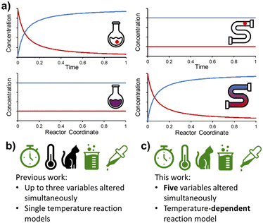
Flow chemistry is conceptually different to its batch counterpart and requires an alternative mindset when designing experiments. Most significantly, the distribution of species in flow is constant over time, but varies in space (Fig. 1a). This is fundamentally different to batch reactions, where (assuming perfect mixing) the distribution of species is constant over space, but varies in time. As a result, a PAT instrument measuring at one position in a flow reactor will only measure a single concentration (assuming the reaction is at steady state), rather than a full reaction time-course. However, with this fundamental difference come new opportunities for reaction design.8
By changing input flow rates, the reaction stream can be treated as a series of pseudo batch reactors, so long as there is minimal influence of axial dispersion.9 Accordingly, when well-designed, such experiments can provide a vast quantity of information for reaction characterization in a short time period, without user intervention. This concept has been exploited by numerous groups in recent years, since the first report in a flow chemistry setting in 2011.10
The group of Jensen reported the first organic chemistry-focused examples9,11 including a recent contribution examining complex non-linear ramps of three variables.12 Wyvratt, McMullen and co-workers have presented the most refined industrial examples, using a combination of FTIR and offline HPLC analysis to simultaneously ramp two parameters.13 They recently also used this approach to optimize a complex objective function for a process and to gain temperature-independent kinetic understanding.14
Bourne used dynamic flow experiments, examining changes in residence time within a single experiment, with a focus on kinetic model generation.15 Recently, Hii reported kinetic model determination for two related substrates at a single temperature by simultaneously varying reagent ratio and total flow rate.16 Numerous other contributions have been made in various fields such as polymer chemistry,17 surfactant synthesis18 and related areas.19
Following on from our earlier foray into the field of dynamic experimentation, which was focused on data processing,20 we endeavored to increase the level of complexity in such experiments. Reports thus far have utilized a maximum of three simultaneous parameter changes (Fig. 1b). In this work, we demonstrate the design of dynamic experiments to rapidly cover a large design space (5 independent variables), and collect the necessary data to build temperature-dependent kinetic models for a catalyzed reaction with two regioisomeric products (Fig. 1c). More complex utilization of this data, by means of flowsheet modeling, is then discussed in the second part of this publication.21
Results and discussion
Reaction of interest and experimental setup
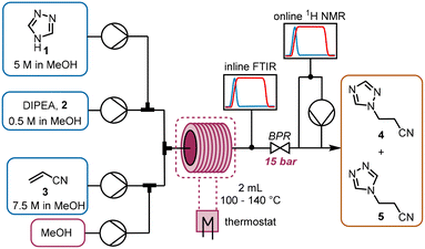
The chemistry scrutinized in this data-driven campaign is a seemingly straightforward Michael addition of 1,2,4-triazole 1 to acrylonitrile 3. It was found that the reaction could be accelerated by base, therefore N,N-diisopropylethylamine (DIPEA, 2) was used in catalytic quantities. As previously reported, this reaction results in two separate products,22 which were found to be regioisomeric products 4 and 5. The similarity of these two products was a key consideration in the PAT strategy. For a scalable process with high productivity, the use of flow chemistry to access high temperature and pressure (high T/p) conditions is highly advantageous.23In order to rapidly perform the reaction in a flexible manner, the flow setup (Fig. 2) consisted of four separate pumps (Knauer, Azura P 4.1S) to deliver three concentrated reagent solutions and a solvent stream. A small volume (2 mL) tubular reactor (Ehrfeld, Hastelloy Capillary Reactor) was used to minimize axial dispersion whilst heating to temperatures up to 140 °C. A back pressure regulator (Zaiput, BPR-10) was set to 15 bar, enabling the reaction to take place at temperatures above the boiling point of the solvent and reagents.24
For analysis of the reaction, two different spectroscopic PAT instruments were proposed: FTIR (Mettler Toledo, ReactIR 15) and NMR25 (Magritek, Spinsolve Ultra 43 MHz). Inline FTIR26 analysis was performed using a pressure-resistant flow cell (SiComp, 50 μL flow cell volume, up to 35 bar), meaning that analysis could be performed before the BPR. Hence, the effect of axial diffusion after the reactor itself was minimal and the reaction progress could be followed closely, with good time resolution for following input changes.
The NMR flow cell (800 μL volume) was not pressure resistant, so the instrument was positioned after the BPR. Furthermore, the NMR measurements are known to be influenced by the flow rate through the cell.25 Therefore, if this instrument were to be used in an inline manner, the range of accessible residence times would be very low (maximum total flow rate ∼1.5 mL min−1). To obviate this problem, a peristaltic pump (Ismatec, ISM834C) was used to sub-sample the stream at a constant flow rate (0.5 mL min−1) for online NMR analysis.
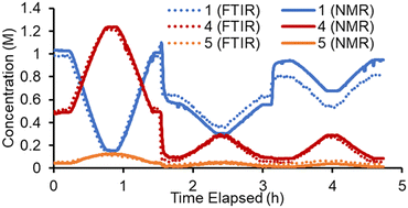
Although the inline FTIR provided a picture of the reaction response to input parameters, it was more challenging to distinguish the different reaction components, due to the similarity between the two isomeric products 4 and 5. However, based on training data (16 concentration levels, with regioisomer ratio determined by benchtop NMR analysis at steady state) a suitable Partial Least Squares (PLS) regression model27 was built, to quantify species 1, 4 and 5 (see ESI† for details). DIPEA 2 and acrylonitrile 3 were difficult to accurately quantify in this model, so were left out.
Conversely, in the online NMR spectra it was possible to partially resolve the two sets of aromatic signals belonging to the two regioisomers 4 and 5. Based on this it was possible to build an Indirect Hard Model (IHM)24,27b to quantify all five species present in the reaction. As previously noted, this technique can be calibrated using only a single experimental point, greatly decreasing the experimental calibration burden. The quantifications from this single point calibration were in good agreement with the FTIR model (Fig. 3). A minor discrepancy in quantity was observed toward the end of the experiment, where starting material 1 was underestimated by the FTIR model. This is thought to be due to the lack of characteristic FTIR signals, which led to poorer quantification. The good agreement of these two measurement techniques (which are at different points along the reactor path) also suggests that the reaction is suitably quenched by simply cooling to room temperature. Although some extent of reaction may occur at room temperature, its influence on the experimental results is expected to be minimal.
Steady state kinetics in flow
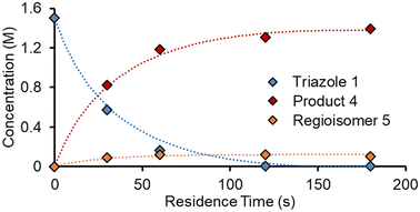
As an initial approach to building a predictive model, a set of sixteen experiments was performed. This was done using the most common current approach for flow experiments, wherein the operator waits for ∼3 residence times for steady state prior to moving to the next experimental conditions. This set comprised four different reaction conditions, each with four residence time points (0.5, 1, 2, 3 min). The resulting dataset required ∼3 h of experimental time and is comparable to running four batch reactions, each with four samples taken along its course.In order to rapidly parameterize a predictive kinetic model, a simplified approach was taken wherein the two reactions (producing major product 4 and side product 5, Fig. 4.) were modeled using the Arrhenius equation, considering all three reaction components (1, 2 and 3). Since DIPEA 2 was not required in stoichiometric quantities, it was treated as a catalytic reagent, which was not consumed in the reaction.
 | (1) |
 | (2) |
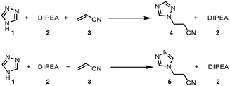 | ||
| Fig. 4 Reaction scheme used for determination of predictive reaction model using Arrhenius kinetics. | ||
At this point it should be stated that the fitted kinetic equation does not aim to provide an accurate representation of the elementary reaction steps in this reaction. To do so would require more complex considerations and ideally data regarding intermediate species, which were not observable here. To simplify the process of building a predictive model, the reactions were treated as single step trimolecular reactions, where non-integer reactant orders between 0.1 and 2 were permitted. Whilst the likelihood of this reaction proceeding via such a reaction pathway is extremely low, the purpose of the model is simply to provide predictions that can be used in future reaction development.
Overall, ten parameters were fitted simultaneously using the software COPASI:28 activation energy, pre-exponential factor and 3× reaction orders for both the major product 4 and regioisomer 5 formation (see eqn (1) and (2)). The measured flow reactor steady state concentrations were averaged over five NMR measurements and treated as individual reaction time points. The fitted model described the experimentally-observed concentrations of species 1, 3, 4 and 5 well (Fig. 5). The identified activation energy parameters were within a reasonable range for both major product 4 and regioisomer 5 (Ea1 = 35.1 kJ mol−1; Ea2 = 38.4 kJ mol−1). Interestingly, the fitted reaction orders (a, b, c) were below 1 for two of the three reactants in each rate equation, but not for the same reactant (b1 = 1.47, a2 = 1.12).
For this dataset, it is likely that the model is overfitted, due to the high number of fitted parameters (10), compared to the relatively small number of data points (16 data points from 4 different reaction conditions). Although this certainly represents a limitation of such a model, employing an overfitted model for comparison purposes within this study was not considered problematic. Furthermore, the reaction model was later tested with a wide range of reaction conditions, where it proved to perform to a satisfactory level. Experimental error may also arise in this approach, due to the slight fluctuations in steady state and the averaging used to take a single value.
Dynamic experiments
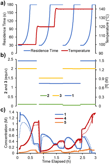
To accelerate the process of gathering the necessary data, the same set of experiments was performed again in flow, but using a dynamic approach. Therein, the total flow rate was ramped for each experiment over a period of 20 min (Fig. 6a), providing residence times between 60 and 180 s. Using the PAT strategy discussed previously (Fig. 2), concentration measurements were obtained at regular intervals, every ∼10 s. This allowed the experiments to be carried out in a similar experimental time of ∼3 h but, perhaps more importantly, provided a high data density of ∼120 points per set of conditions.To fit a similar predictive model as in the steady state experiments, a MatLab script was written in which the reaction input was discretized into segments of ∼10 s (aligned with NMR measurements). These segments were approximated as individual batch reactors, and their composition tracked by a standard batch kinetics approach, using ordinary differential equations, as they progressed through the reactor.19 This approach allowed each segment to experience different temperatures whilst travelling through the reactor, making it compatible with temperature ramps. The composition at the measurement point was then predicted and compared to the measured values. Dispersion in the system was simulated using the lsim tool with a continuous-time transfer function.
The model was parameterized using a bounded Nelder–Mead optimizer in MatLab (fminsearchbnd), aiming to minimize the normalized root mean square error (RMSE) of the four measured components (with equal weighting). Due to the large number of data points and parameters to fit, the parameterization was relatively slow (duration ∼16 h), but provided a low average RMSE of 5.17% for this experiment. As can be observed in the concentration plot (Fig. 6c) there is generally excellent agreement between the predicted and measured values for the components. Where disparity is observed, it appears to be characterized by a shift in time, rather than a difference in the overall prediction. This implies that the main downside of this model is its accounting for the reactor dynamics, rather than the kinetic model itself.
Rapid kinetic modeling using multiple ramps
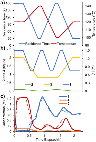
Finally, it was envisaged that a suitable predictive model could be built using a single set of experimental ramps. An experiment was planned in which all five parameters were ramped in a linear manner over ∼2.3 h operating time (Fig. 7). The adjusted parameters were: 1) reaction concentration (0.75–1.5 M); 2) residence time (30–180 s); 3) reaction temperature (100–140 °C); 4) acrylonitrile 3 loading (0.8–2.0 equiv.); 5) DIPEA 2 loading (0.01–0.10 equiv.). The variable ramps were designed to be out of phase with one another to maximize the variation and range of condition combinations accessed. Using the same approach as described above, the reaction parameters were fitted. The smaller quantity of data meant that this process was now substantially faster (∼8 h) and resulted in a similar RMSE of 5.38%.Reaction model comparison
To compare the effectiveness of each experimental approach, a number of additional experiments were used as validation data sets (Table 1). In each of the experiments different combinations of parameter ramps were examined. Experiment 1 comprises the four residence time ramps (discussed above in the “Dynamic experiments” section). Experiment 2 contained only temperature ramps, with the other parameters held constant at 3 different levels. In experiment 3 one reagent concentration was ramped at a time, then combined with a temperature ramp. From experiment 4 onwards multiple parameters were ramped simultaneously: two, three, four or five parameters in experiments 4, 5, 6 and 7, respectively. Full details for each experiment are available in the ESI.†| Experiment | Steady state RMSE [1]a | Dynamic RMSE [1]a | Multi-ramp RMSE [7]a |
|---|---|---|---|
| RMSE is calculated as a relative value, normalized versus the maximum observed concentration for each species. The value presented is the mean RMSE for all species 1, 3, 4 and 5.a The experiment set that was used to parameterize each model is shown in square brackets and highlighted in bold. | |||
| 1 | 6.30% | 5.17% | 7.77% |
| 2 | 10.08% | 9.24% | 10.10% |
| 3 | 8.09% | 8.60% | 7.15% |
| 4 | 11.83% | 12.74% | 8.74% |
| 5 | 10.16% | 10.92% | 7.60% |
| 6 | 9.14% | 9.13% | 6.58% |
| 7 | 6.27% | 6.74% | 5.38% |
| Mean | 8.83% | 8.93% | 7.62% |
When comparing the performance of the differently parameterized models, the “multi-ramp” variant (trained using experiment 7) was superior for all validation experiments (with the exception of experiment 2). It should be expected that the model's own parameterization experiment provides the lowest RMSE, therefore the observed performance in experiment 1 is unsurprising.
There are numerous potential sources of error that likely contribute to these RMSE values. First and foremost, the model does not take into account reactor dynamics, meaning that the trace for measured vs. predicted results are often misaligned. Additionally, small variations in reaction solution concentrations and pump flow rates may contribute to overall errors. Finally, the chemometric model (IHM) inherently has error associated, particularly at low concentrations, which has an influence in both model fitting experiments and validation experiments.
Reaction model validation
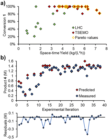
In order to validate the kinetic model on an entirely different data set, a self-optimization experiment was carried out using the same reactor system. The Thompson Sampling Efficient Multi-objective Optimization (TSEMO) algorithm, pioneered in a chemistry environment by Schweidtmann, Bourne and Lapkin,29 was used to optimize three objectives: conversion, space–time yield and E-factor. These objectives were chosen to provide a spread of experimental setpoints, focused toward high extent of reaction, high throughput and low waste, respectively.All five variables that were ramped in the initial experiments were included as optimizable variables: 1) reaction concentration; 2) residence time; 3) reaction temperature; 4) acrylonitrile 3 loading; 5) DIPEA 2 loading. The experiments were, however, carried out as steady state reactions, by setting initial parameters and waiting for steady state to be reached (i.e. not as dynamic experiments). The self-optimization was initiated with a Latin hypercube (LHC) set of 10 experiments (2n, where n is the number of optimizable variables). Thereafter, 28 optimization experiments were performed, providing a dataset of 38 experiments.
After the initial LHC experiments, the TSEMO algorithm rapidly began to define a pareto front at complete conversion (Fig. 8a), which was relatively straightforward to achieve. Maximizing the space–time yield was then explored, where higher values were achieved at incomplete conversion. A maximum space–time yield of 7.37 kg L−1 h−1 was observed, where the reaction operated at only 82% conversion.
The measured values from these steady state experiments were then compared with the predictions from the simple kinetic model, parameterized using MatLab. Gratifyingly, there was excellent agreement between the predicted and measured values for triazole 1, acrylonitrile 3 and main product 4. The relative RMSE for these were 3.8%, 5.7% and 5.2%, respectively.
The measured and predicted values for main product 4 (Fig. 8b) are of particular interest, showing good parity between all points, aside from two outliers (consecutive experiments 31 and 32, where product is significantly over-predicted).
The relative RMSE for the side product 5 was far poorer than the other three components, at 27.9%. However, this was likely, in part, due to the lower concentrations involved (up to 0.13 M, c.f. ∼1.4 M for main product 4). The absolute RMSE is 38 mM (c.f. 72 mM for main product 4), which will be influenced by compound error in the chemometric model, pump flow rates and other factors.
With this validated model in hand, it should be noted that further in silico optimization can be performed, without experimental effort. For example, the same TSEMO multi-objective algorithm can be carried out with a far larger experiment set, allowing the pareto front to be fully defined in a short time period (see ESI†).
As previously discussed, the reactor dynamics are poorly accounted for using this modeling approach. Therefore, more complex corrections or alternative methods may be advantageous. In the accompanying manuscript, a flowsheet modeling approach with dispersion correction is presented and discussed in detail for the same reaction.21
Conclusions
We have described a workflow for rapidly exploring a reaction in flow, making use of the possibility to screen numerous different reaction parameters within a single experiment. A kinetic model parameterized using a multi-ramp flow experiment (5 variables altered simultaneously) proved to provide more effective predictions than simpler experiments and required a shorter experimental time. External validation against a self-optimization experiment was also successful, thereby the resulting model could be used for in silico optimization as well as further development and scale-up.Data availability
The experimental data generated during this study can be found online at: https://doi.org/10.5281/zenodo.7829130.Conflicts of interest
There are no conflicts to declare.Acknowledgements
The authors gratefully acknowledge funding by Land Steiermark/Zukunftsfonds Steiermark (No. 9003) for acquiring the infrastructure used in this work. The Research Center Pharmaceutical Engineering (RCPE) is funded within the framework of COMET – Competence Centers for Excellent Technologies by BMK, BMDW, Land Steiermark and SFG. The COMET program is managed by the FFG.Notes and references
- For discussion of data-rich labs, see:
(a) S. Caron and N. M. Thomson, J. Org. Chem., 2015, 80, 2943–2958 CrossRef CAS PubMed
; (b) L. Wilbraham, S. H. M. Mehr and L. Cronin, Acc. Chem. Res., 2021, 54, 253–262 CrossRef CAS PubMed
; (c) B. Mahjour, Y. Shen and T. Cernak, Acc. Chem. Res., 2021, 54, 2337–2346 CrossRef CAS PubMed
.
- For selected articles discussing high throughput experimentation (HTE) in batch, see:
(a) M. Shevlin, ACS Med. Chem. Lett., 2017, 8, 601–607 CrossRef CAS PubMed
; (b) N. S. Eyke, B. A. Koscher and K. F. Jensen, Trends Chem., 2021, 3, 120–132 CrossRef CAS
; (c) S. A. Biyani, Y. W. Moriuchi and D. H. Thompson, Chem.: Methods, 2021, 1, 323–339 CAS
; (d) L. Buglioni, F. Raymenants, A. Slattery, S. D. A. Zondag and T. Noël, Chem. Rev., 2022, 122, 2752–2906 CrossRef CAS PubMed
; (e) M. Christensen, L. P. E. Yunker, P. Shiri, T. Zepel, P. L. Prieto, S. Grunert, F. Bork and J. E. Hein, Chem. Sci., 2021, 12, 15473–15490 RSC
.
- For selected examples exploiting large volumes of data from batch synthetic chemistry experiments, see:
(a) D. T. Ahneman, J. G. Estrada, S. Lin, S. D. Dreher and A. G. Doyle, Science, 2018, 360, 186–190 CrossRef CAS PubMed
; (b) B. J. Shields, J. Stevens, J. Li, M. Parasram, F. Damani, J. I. M. Alvarado, J. M. Janey, R. P. Adams and A. G. Doyle, Nature, 2021, 590, 89–96 CrossRef CAS PubMed
; (c) Y. Shi, P. L. Prieto, T. Zepel, S. Grunert and J. E. Hein, Acc. Chem. Res., 2021, 54, 546–555 CrossRef CAS PubMed
; (d) M. Fitzner, G. Wuitschik, R. Koller, J.-M. Adam and T. Schindler, ACS Omega, 2023, 8, 3017–3025 CrossRef CAS PubMed
.
- For discussion of quality by design in pharmaceutical development, see:
(a) L. X. Yu, Pharm. Res., 2008, 25, 781–791 CrossRef CAS PubMed
; (b) A. A. Zlota, Org. Process Res. Dev., 2022, 26, 899–914 CrossRef CAS
.
- For selected reviews of data-rich flow chemistry, see:
(a) B. J. Reizman and K. F. Jensen, Acc. Chem. Res., 2016, 49, 1786–1796 CrossRef CAS PubMed
; (b) D. E. Fitzpatrick, C. Battilocchio and S. V. Ley, ACS Cent. Sci., 2016, 2, 131–138 CrossRef CAS PubMed
; (c) A. A. Volk and M. Abolhasani, Trends Chem., 2021, 3, 519–522 CrossRef CAS
; (d) R. W. Epps, A. A. Volk, M. Y. S. Ibrahim and M. Abolhasani, Chem, 2021, 7, 2541–2545 CrossRef CAS
.
- For selected reviews of self-optimizing reactions in flow, see:
(a) A. D. Clayton, J. A. Manson, C. J. Taylor, T. W. Chamberlain, B. A. Taylor, G. Clemens and R. A. Bourne, React. Chem. Eng., 2019, 4, 1545–1554 RSC
; (b) C. Mateos, M. J. Nieves-Remacha and J. A. Rincón, React. Chem. Eng., 2019, 4, 1536–1544 RSC
; (c) C. J. Taylor, A. Pomberger, K. C. Felton, R. Grainger, M. Barecka, T. W. Chamberlain, R. A. Bourne, C. N. Johnson and A. A. Lapkin, Chem. Rev., 2023, 123, 3089–3126 CrossRef CAS PubMed
.
- For selected reviews of PAT in flow, see:
(a) M. A. Morin, W. Zhang, D. Mallik and M. G. Organ, Angew. Chem., Int. Ed., 2021, 60, 20606–20626 CrossRef CAS PubMed
; (b) M. Rodriguez-Zubiri and F.-X. Felpin, Org. Process Res. Dev., 2022, 26, 1766–1793 CrossRef CAS
.
- C. J. Taylor, J. A. Manson, G. Clemens, B. A. Taylor, T. W. Chamberlain and R. A. Bourne, React. Chem. Eng., 2022, 7, 1037–1046 RSC
.
- J. S. Moore and K. F. Jensen, Angew. Chem., Int. Ed., 2014, 53, 470–473 CrossRef CAS PubMed
.
- S. Mozharov, A. Nordon, D. Littlejohn, C. Wiles, P. Watts, P. Dallin and J. M. Girkin, J. Am. Chem. Soc., 2011, 133, 3601–3608 CrossRef CAS PubMed
.
- B. J. Reizman and K. F. Jensen, Org. Process Res. Dev., 2012, 16, 1770–1782 CrossRef CAS
.
- F. Florit, A. M. K. Nambiar, C. P. Breen, T. F. Jamison and K. F. Jensen, React. Chem. Eng., 2021, 6, 2306–2314 RSC
.
- B. M. Wyvratt, J. P. McMullen and S. T. Grosser, React. Chem. Eng., 2019, 4, 1637–1645 RSC
.
- J. P. McMullen and B. M. Wyvratt, React. Chem. Eng., 2022, 8, 137–151 RSC
.
-
(a) C. A. Hone, N. Holmes, G. R. Akien, R. A. Bourne and F. L. Muller, React. Chem. Eng., 2017, 2, 103–108 RSC
; (b) C. J. Taylor, M. Booth, J. A. Manson, M. J. Willis, G. Clemens, B. A. Taylor, T. W. Chamberlain and R. A. Bourne, Chem. Eng. J., 2021, 413, 127017 CrossRef CAS
.
- L. Schrecker, J. Dickhaut, C. Holtze, P. Staehle, M. Vranceanu, K. Hellgardt and K. K. Hii, React. Chem. Eng., 2023, 8, 41–46 RSC
.
- J. Van Herck and T. Junkers, Chem.: Methods, 2022, 2, 1–6 Search PubMed
.
- R. J. T. Kleijwegt, V. C. Henricks, W. Winkenwerder, W. Baan and J. Van Der Schaaf, React. Chem. Eng., 2021, 6, 2125–2139 RSC
.
-
(a) C. Waldron, A. Pankajakshan, M. Quaglio, E. Cao, F. Galvanin and A. Gavriilidis, React. Chem. Eng., 2020, 5, 112–123 RSC
; (b) C. Waldron, A. Pankajakshan, M. Quaglio, E. Cao, F. Galvanin and A. Gavriilidis, Ind. Eng. Chem. Res., 2019, 58, 22165–22177 CrossRef CAS
; (c) C. Waldron, A. Pankajakshan, M. Quaglio, E. Cao, F. Galvanin and A. Gavriilidis, React. Chem. Eng., 2019, 4, 1623–1636 RSC
.
- P. Sagmeister, J. Poms, J. D. Williams and C. O. Kappe, React. Chem. Eng., 2020, 5, 677–684 RSC
.
- For the second part of this manuscript, entitled “Accelerating Reaction Modeling Using Dynamic Flow Experiments, Part 2: Development of a Digital Twin”, see: K. Silber, P. Sagmeister, C. Schiller, J. D. Williams, C. A. Hone and C. O. Kappe, React. Chem. Eng. 10.1039/D3RE00244F
.
- K. Kodolitsch, F. Gobec and C. Slugovc, Eur. J. Org. Chem., 2020, 2973–2978 CrossRef CAS
.
- For selected reviews discussing high temperature and pressure chemistry, see:
(a) T. N. Glasnov and C. O. Kappe, Chem. – Eur. J., 2011, 17, 11956–11968 CrossRef CAS PubMed
; (b) V. Hessel, D. Kralisch, N. Kockmann, T. Noël and Q. Wang, ChemSusChem, 2013, 6, 746–789 CrossRef CAS PubMed
.
- For previous examples of a similar reactor setup and methodology, see:
(a) S. Knoll, C. E. Jusner, P. Sagmeister, J. D. Williams, C. A. Hone, M. Horn and C. O. Kappe, React. Chem. Eng., 2022, 7, 2375–2384 RSC
; (b) P. Sagmeister, F. F. Ort, C. E. Jusner, D. Hebrault, T. Tampone, F. G. Buono, J. D. Williams and C. O. Kappe, Adv. Sci., 2022, 9, 2105547 CrossRef PubMed
.
- P. Giraudeau and F. X. Felpin, React. Chem. Eng., 2018, 3, 399–413 RSC
.
- T. Brodmann, P. Koos, A. Metzger, P. Knochel and S. V. Ley, Org. Process Res. Dev., 2012, 16, 1102–1113 CrossRef CAS
.
- For selected studies using PLS modelling for flow reactions, see:
(a) Y. Miyai, A. Formosa, C. Armstrong, B. Marquardt, L. Rogers and T. Roper, Org. Process Res. Dev., 2021, 25, 2707–2717 CrossRef CAS
; (b) P. Sagmeister, R. Lebl, I. Castillo, J. Rehrl, J. Kruisz, M. Sipek, M. Horn, S. Sacher, D. Cantillo, J. D. Williams and C. O. Kappe, Angew. Chem., 2021, 60, 8139–8148 CrossRef CAS PubMed
; (c) P. Sagmeister, D. Kaldre, J. Sedelmeier, C. Moessner, K. Püntener, D. Kummli, J. D. Williams and C. O. Kappe, Org. Process Res. Dev., 2021, 25, 1206–1214 CrossRef CAS
.
- S. Hoops, R. Gauges, C. Lee, J. Pahle, N. Simus, M. Singhal, L. Xu, P. Mendes and U. Kummer, Bioinformatics, 2006, 22, 3067–3074 CrossRef CAS PubMed
.
- For selected studies using the TSEMO algorithm, see:
(a) E. Bradford, A. M. Schweidtmann and A. Lapkin, J. Glob. Optim., 2018, 71, 407–438 CrossRef
; (b) A. M. Schweidtmann, A. D. Clayton, N. Holmes, E. Bradford, R. A. Bourne and A. A. Lapkin, Chem. Eng. J., 2018, 352, 277–282 CrossRef CAS
; (c) A. D. Clayton, A. M. Schweidtmann, G. Clemens, J. A. Manson, C. J. Taylor, C. G. Niño, T. W. Chamberlain, N. Kapur, A. J. Blacker, A. A. Lapkin and R. A. Bourne, Chem. Eng. J., 2020, 384, 123340 CrossRef CAS
.
Footnote |
| † Electronic supplementary information (ESI) available: Additional experimental details and results. See DOI: https://doi.org/10.1039/d3re00243h |
| This journal is © The Royal Society of Chemistry 2023 |

