Autonomous kinetic model identification using optimal experimental design and retrospective data analysis: methane complete oxidation as a case study†
Received
16th March 2023
, Accepted 14th June 2023
First published on 30th June 2023
Abstract
Automation and feedback optimization are combined in a smart laboratory platform for the purpose of identifying appropriate kinetic models online. In the platform, model-based design of experiments methods are employed in the feedback optimization loop to design optimal experiments that generate data needed for rapid validation of kinetic models. The online sequential decision-making in the platform, involving selection of the most appropriate kinetic model structure followed by the precise estimation of its parameters, is done by autonomously switching the respective objective functions to discriminate between competing models and to minimise the parametric uncertainty of an appropriate model. The platform is also equipped with data analysis methods to study the behaviour of models within their uncertainty limits. This means that the platform not only facilitates rapid validation of kinetic models, but also returns uncertainty-aware predictive models that are valuable tools for model-based decision systems. The platform is tested on a case study of kinetic model identification of complete oxidation of methane on a Pd/Al2O3 catalyst, employing a micro-packed bed reactor. A suitable kinetic model with precise estimation of its parameters was determined by performing a total of 20 automated experiments, completed in two days.
1 Introduction
The fast-proceeding digitalisation in process industries has led to the automation of decision-making processes in plant operations. This involves optimizations with high-fidelity and data-driven models that are continuously validated using data generated through feedback optimization loops. In the context of automated decision-making in chemical processes, decision-making often involves optimizations with high-fidelity kinetic models. Combining flow chemistry,1 microreactor technology2,3 and computational methods has provided automated platforms for rapid development and identification of kinetic models. The methods employed in automated platforms for the development of kinetic models of chemical reactions fall into two categories: i) automated mechanism generation and model building and ii) automated model validation and refinement.
Some of the notable contributions in the first category include the reaction modelling suite (RMS),4 reaction mechanism generator (RMG)5,6 and Genesys.7,8 All these studies propose tools to automatically translate a set of chemistry rules into model equations and to validate the resultant models. A similar approach used for discovery of new synthetic routes is computer aided synthesis planning (CASP) which is a machine learning-assisted optimized search methodology to find feasible routes towards a target molecule, given the target molecule as the input.9–11 In general, the automatic generation of chemical reaction mechanisms and kinetic model structures using brute-force computing algorithms subjected to feasibility constraints will eventually reduce the redundant task of chemists or modellers in scripting down the model equations. It will also improve the level of knowledge abstraction between similar systems.
The second category of methods is focused on the automated validation of mechanistic or data-driven process models in smart laboratory platforms integrated with intelligent design with (closed loop) or without (open loop) feedback optimization. Significant contribution in this research field includes self-optimizing reaction systems12–16 that mainly use design of experiments (DoE) methods17–19 and regression models to optimize the process conditions in automated flow reactor systems. Another approach includes application of online model-based design of experiments (MBDoE) methods20,21 in automated reactor platforms to optimally explore the design space to generate information-rich data needed for rapid validation of mechanistic kinetic models.22–30
In this work, we report the development of an algorithmic and computational framework to achieve autonomous kinetic model identification in a smart microreactor platform for a heterogeneously catalysed gas/solid reaction. Here, the keyword smart means that the microreactor system is fully automated and digitalised for our purpose and the keyword autonomous is used to indicate that the platform is self-sufficient to identify and study appropriate kinetic models without any human intervention. Although similar platforms have been previously reported and successfully applied to solve real world problems of chemical kinetics,24,28 in this work, we propose a framework in which the autonomous features necessary for kinetic model identification are powered by optimal experimental design and retrospective analysis of models. Another intention of this paper is to report a new Python optimization modeling object (Pyomo)31–33 based parameter estimation module and a probability criterion for online model selection, both part of the proposed framework. This paper is organised as follows: i) in section 2, the main modules of the smart laboratory platform with the theoretical details are discussed, ii) section 3 introduces the case study of complete oxidation of methane along with the details of candidate kinetic models and the model reparameterisations used, iii) section 4 discusses the results obtained and the major implications, and iv) section 5 provides a conclusion and future scope of the work.
2 Methods
The flowchart of the algorithmic and computational framework of the smart laboratory platform used for autonomous identification of kinetic models is shown in Fig. 1. As shown in the figure, the platform is driven by a computational framework consisting of five modules: 1) preliminary design module, 2) resource module, 3) model calibration module, 4) autonomous decision module, and 5) model-based design of experiments module. These five modules are operated in a loop until the goal of identifying a predictive kinetic model is achieved. An add-on to the platform is the retrospective data analysis module, which has been set up to review the results obtained by the platform, to reassess the decisions taken by the platform and to provide further insights or actions if needed.
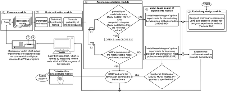 |
| | Fig. 1 Flowchart of the computational framework employed in the smart laboratory platform for online kinetic studies. | |
2.1 Preliminary design module
The preliminary design module consists of pure statistical (model-free) DoE methods whose objective is to efficiently sample the experimental design space (the domain of possible values of the experimental conditions) for qualitative and quantitative purposes. The first qualitative purpose of DoE methods is to provide randomisation of experiments, meaning that the experimental conditions must be independent of each other and should represent the entire design space. This is necessary to protect the principal assumption in estimation methods that the output data is a random sample of some infinite population that describes the whole characteristic of the system. Further qualitative benefits from DoE methods are: i) greater efficiency, meaning that the experimental sampling should provide more information about the system with less experiments, and ii) greater comprehensiveness, which means that the DoE sampling should result in experiments that help to understand the whole of the cause–effect relationships of the system.17 The quantitative purpose of DoE sampling is to generate output data to be used for i) estimating the random error in observations, possibly from a few repetitions of some experiments, and ii) the primary validation of the proposed process models, i.e., to obtain an estimate of the model parameters and their statistical uncertainty. The latter is important in the robustness of the step of designing model-based optimal experiments, which is explained in the design module of the platform. As shown in Fig. 1, in this work, factorial17 DoE is used in the preliminary design module. The factorial arrangement of experiments, in which the causing factors or inputs are varied over different discrete levels and the experiments consist of all possible combinations of these levels across all the factors, offers all the significant advantages stated above. However, one disadvantage of using a factorial design is the explosive growth of experiments with increasing number of factors and levels. As a solution, in higher dimensional experimental design space, two-level fractional factorial designs remain the preferred choice.34 A generalised version of the traditional fractional factorial designs is the generalized subset design (GSD),34 which is appropriate for problems where factors have more than two levels.
2.2 Resource module
The execution of actual experiments in the smart laboratory platform will generate output data that are used to validate the set of proposed process models (the set of models corresponding to different hypothesised reaction mechanisms). The proposed reaction process models are called identification models. The data together with the set of identification models comprise the resource module of the smart laboratory platform (see Fig. 1). The identification models of chemical reaction systems are commonly differential and algebraic equations (DAEs), which can be represented in the following state-space form| |  | (1) |
In eqn (1), x ∈ ![[Doublestruck R]](https://www.rsc.org/images/entities/char_e175.gif) Nx is the vector of state variables, ẋ is the vector of first derivatives of the state variables, u ∈
Nx is the vector of state variables, ẋ is the vector of first derivatives of the state variables, u ∈ ![[Doublestruck R]](https://www.rsc.org/images/entities/char_e175.gif) Nu is the vector of inputs or control variables that define the condition of an experiment, θ ∈
Nu is the vector of inputs or control variables that define the condition of an experiment, θ ∈ ![[Doublestruck R]](https://www.rsc.org/images/entities/char_e175.gif) Nθ is the vector of model parameters, ŷ ∈
Nθ is the vector of model parameters, ŷ ∈ ![[Doublestruck R]](https://www.rsc.org/images/entities/char_e175.gif) Nŷ is the vector of model predictions of the outputs or response variables y (those state variables which are measured), f denotes the vector of functions representing the state equation and h denotes a function selecting the set of state variables representing measured outputs. In the case of chemical reaction systems, both f and h are usually nonlinear functions of θ and u. The outputs y from different experiments result in a population of data which can be learnt by repeating some experiments and calculating means and standard errors. The common practice is to assume that the measurement error ε follows an independent and identically distributed (i.i.d) Gaussian distribution with mean vector 0 and covariance matrix Σy, which are then calculated from repeated experiments. We have also followed this approach here and more details about this can be found in our previous work.35
Nŷ is the vector of model predictions of the outputs or response variables y (those state variables which are measured), f denotes the vector of functions representing the state equation and h denotes a function selecting the set of state variables representing measured outputs. In the case of chemical reaction systems, both f and h are usually nonlinear functions of θ and u. The outputs y from different experiments result in a population of data which can be learnt by repeating some experiments and calculating means and standard errors. The common practice is to assume that the measurement error ε follows an independent and identically distributed (i.i.d) Gaussian distribution with mean vector 0 and covariance matrix Σy, which are then calculated from repeated experiments. We have also followed this approach here and more details about this can be found in our previous work.35
2.3 Model calibration module
The objective of the model calibration module is to test if the identification models can represent the population of output data, i.e., to check if the models are able to describe the output data and their distribution. As seen in Fig. 1, this module involves three classes of methods: i) parameter estimation, ii) statistical hypothesis testing and iii) model selection by means of probability of model adequacy.
2.3.1 Parameter estimation.
In the parameter estimation step, the identification models are used to fit the output data with the objective to estimate the unknown parameters of these models for which the models are able to describe the data within the limits of their learnt population. In this work, we have used the method of maximum likelihood36,37 for parameter estimation. This method suggests that the most probable values of the model parameters are those that maximise the likelihood function ![[script L]](https://www.rsc.org/images/entities/char_e144.gif) (θ|Y) given below
(θ|Y) given below| |  | (2) |
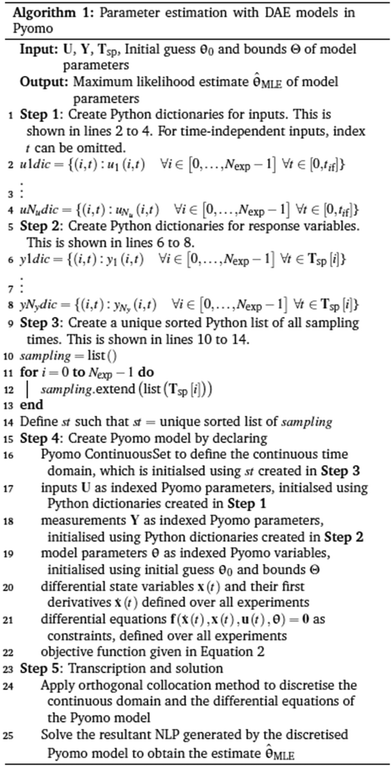
Note that the form of likelihood function provided in eqn (2) is based on the earlier assumptions ε ∼ ![[scr N, script letter N]](https://www.rsc.org/images/entities/char_e52d.gif) (0, Σy) made about the measurement error distribution. In eqn (2), Y denotes the entire set of output data, p(·) denotes the probability density function and n denotes the total number of samples. As mentioned in section 2.2, since f is usually nonlinear in θ, often the parameter estimation problems are nonlinear and nonconvex optimization problems with multiple local optima, sometimes including flat regions in the objective function because of poor parameter identifiability.38–40 The effective solution of the parameter estimation problems with a fast and good convergence is critical in online estimation methods. To tackle this, in this work, we have solved the parameter estimation problems using a code developed in Pyomo.31–33 This implementation is particularly suited for solving parameter estimation with models represented by DAEs. The algorithm of this implementation is provided in Algorithm 1.
(0, Σy) made about the measurement error distribution. In eqn (2), Y denotes the entire set of output data, p(·) denotes the probability density function and n denotes the total number of samples. As mentioned in section 2.2, since f is usually nonlinear in θ, often the parameter estimation problems are nonlinear and nonconvex optimization problems with multiple local optima, sometimes including flat regions in the objective function because of poor parameter identifiability.38–40 The effective solution of the parameter estimation problems with a fast and good convergence is critical in online estimation methods. To tackle this, in this work, we have solved the parameter estimation problems using a code developed in Pyomo.31–33 This implementation is particularly suited for solving parameter estimation with models represented by DAEs. The algorithm of this implementation is provided in Algorithm 1.
Parameter estimation using DAEs in Pyomo involves discretisation transformation of the DAEs into algebraic equations and then solving the parameter estimation problem using the discretised models. The transformation of DAEs into algebraic equations is done by discretisation of the continuous domain of the DAEs and defining equality constraints to approximate derivatives at the discretisation points. In this work, orthogonal collocation41 is used to discretise the continuous domain in the DAEs. It shall be noted that the algorithm for solving the parameter estimation problem in Pyomo is presented for the general case of DAEs integrated over time (i.e., time t is treated as the independent variable that also defines the continuous domain) and the response variables measured at different time points, which are the sampling times. This should not restrict the application of the algorithm to the cases of DAEs integrated over reactor length or other continuous domains and the response variables measured at a specific sensor location or at a steady state time.
| |  | (3) |
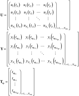
As shown in Algorithm 1, steps 1 and 2 of the algorithm involve developing helper functions to create Python dictionaries for defining inputs and outputs in the Pyomo model. Step 3 involves creating a sorted Python list of all sampling times, which is needed to define the discretisation points in the Pyomo model. The full set of inputs
U, outputs
Y and sampling times
Tsp from all the performed experiments which are needed in steps 1–3 of the algorithm are provided as Python lists as given in
eqn (3). Step 4 of the algorithm involves developing the Pyomo model using the inputs, outputs and sampling times created in steps 1–3. The final step 5 involves the discretisation of the Pyomo model and the solution of the resulting nonlinear programming (NLP) problem to obtain the maximum likelihood estimates
![[small straight theta, Greek, circumflex]](https://www.rsc.org/images/entities/b_char_e12d.gif) MLE
MLE of model parameters.
2.3.2 Statistical hypothesis testing.
In this sub-module, methods of statistical hypothesis testing17,42,43 are used to test the validity of the results of parameter estimation. Two statistical hypothesis tests are used to validate the results of parameter estimation. The first test is the chi-square goodness of fit test,44 which is used to test whether the errors of fitting confirm or contradict the hypothesis of randomly distributed measurement errors ε. For this purpose, the test evaluates whether the distribution of residuals (y − ŷ) can be considered as a random sample of the specified error distribution ε ∼ ![[scr N, script letter N]](https://www.rsc.org/images/entities/char_e52d.gif) (0, Σy). The test is performed by computing the chi-square χ2 statistic according to the equation
(0, Σy). The test is performed by computing the chi-square χ2 statistic according to the equation| |  | (4) |
and comparing the computed value to the reference chi-square value  , which is the value from a chi-square distribution with (N − Nθ) degrees of freedom and an α significance level. Here, N represents the total number of observations, i.e., N = n·Ny. If the computed chi-square value is greater than the reference value, the deviations (y − ŷ) are greater than twice the standard deviation of the error distribution and hence the model fails to describe the data. Otherwise, the model is regarded as an adequate representation of the data. The second test is Student's t-test,45 which is used to evaluate the statistical quality of parameter estimates. The aim of the test is to confirm from data whether the variation in the parameter estimates is contradicted or explained by the variation within the data. The variation in the parameter estimates can be explained using the parameter covariance matrix Vθ which is approximated as the inverse of observed Fisher information matrix (FIM) Hθ, which in turn is approximated as
| |  | (5) |
In eqn (5), V0θ is the prior covariance matrix and  is the Ny × Nθ parameter sensitivity matrix whose elements are the sensitivity coefficients that are first derivatives of dependent variables w.r.t model parameters. From the parameter covariance matrix, the test statistic t-value for Student's t-test can be computed for each parameter estimate as
| |  | (6) |
In eqn (6), ![[small straight theta, Greek, circumflex]](https://www.rsc.org/images/entities/b_char_e12d.gif) i is the estimate of the i-th model parameter, the denominator of the equation represents (1 − α) 100% confidence interval around the parameter estimates and Vθii denotes the i-th diagonal element of the parameter covariance matrix. In Student's t-test, the computed t-value of the individual model parameter is compared to a reference value tref = tN−Nθ(1 − α/2), which is the t-value from a two-tailed t-distribution with (N – Nθ) degrees of freedom and an α significance level. For a parameter estimate having a large confidence interval compared to the estimated value, the computed t-statistic tends to be smaller than the reference value and the estimation of that parameter is not considered statistically precise. Parameters having t-values larger than the reference values are considered well estimated. Another important factor to consider while investigating the quality of parameter estimates is the parameter correlation matrix Cθ whose elements are defined by
i is the estimate of the i-th model parameter, the denominator of the equation represents (1 − α) 100% confidence interval around the parameter estimates and Vθii denotes the i-th diagonal element of the parameter covariance matrix. In Student's t-test, the computed t-value of the individual model parameter is compared to a reference value tref = tN−Nθ(1 − α/2), which is the t-value from a two-tailed t-distribution with (N – Nθ) degrees of freedom and an α significance level. For a parameter estimate having a large confidence interval compared to the estimated value, the computed t-statistic tends to be smaller than the reference value and the estimation of that parameter is not considered statistically precise. Parameters having t-values larger than the reference values are considered well estimated. Another important factor to consider while investigating the quality of parameter estimates is the parameter correlation matrix Cθ whose elements are defined by| |  | (7) |
If Cij approaches 1, parameters are highly correlated (or −1 for anti-correlated), which makes their unique estimation difficult. In the case of perfect correlation Cij = 1 or anti-correlation Cij = −1, one parameter can be expressed as a function of the other. This will alter the degrees of freedom and cause the t-test to be invalid.
2.3.3 Probability of model adequacy.
In this sub-module, a probability criterion is proposed to assign probabilities to models based on their relative fitting quality. The need for defining such a probability criterion is to select the best model in situations where more than one model appears to be compatible with the same set of observations; a situation referred to as equifinality46 or model indeterminacy by modellers.47 A possible example of model indeterminacy in chemical systems can happen in kinetic models of heterogeneous chemical reactions involving adsorption of a gas on a metal oxide catalyst surface.48 In such systems, the adsorption is affected by the source of the gas and the catalytic properties of the exposed surface and in many cases a distinction between types of adsorption (dissociative or molecular) is less clear from observed concentration data. Even when the distinction is clear at the atomic scale or surface level, the observed similar behaviour in the bulk phase (use of error prone concentration measurements from the bulk phase) can render any validation or discrimination attempt between different models based on the type of adsorption impossible.48 Under such circumstances, using statistics for online model selection or discrimination appears a vague index, but the equivalent probability represents a clear and user-friendly index.49 The probability of model adequacy proposed in this work is defined as| |  | (8) |
In eqn (8), Prj is the probability not to reject model j, assuming that the null hypothesis that the distribution of residuals of model j is a random sample of the error distribution is true. The probabilities Pr(·) in the numerator and denominator of the equation are the p-value of the chi-square goodness of fit test. The greater these probability values, the more points in the residual distribution are not contradicted by the distribution of the measurement error. In this work, a target probability of 90% is set as the threshold probability to select the most appropriate kinetic model.
2.4 Autonomous decision module
In this module, the results of parameter estimation, statistical hypothesis testing and the probability criterion are combined to make inferences regarding different identification models. The module contains two case (if–else) statements that are used to make decisions in the identification procedure. As shown in Fig. 1, the two case statements are connected in parallel using switches S1 and S2. By default, S1 is closed and S2 is open. Hence, the first decision is made regarding the adequacy of identification models based on the results of the chi-square goodness of fit test and values of probability of model adequacy. When this condition is met, satisfying the threshold values of both the chi-square goodness of fit test and values of probability of model adequacy, an appropriate model that is able to represent the data has been selected from the set of identification models. This will automatically make the switch S1 open and S2 closed. Therefore, the second case statement to analyse the statistical precision of parameter estimates becomes activated. In the second case statement, the t-values of model parameters are used to assess if the parameters of the selected model (the model with the highest probability value) are precisely estimated. The case statement asks for more evidence or data when the condition is not met or sends a termination command if the condition is met.
2.5 Model-based design of experiments module
In the event of limitation of evidence to make inferences from the autonomous decision module i.e., when the conditions in the autonomous decision module are not met, future experiments are optimally designed using MBDoE methods. This is the job of the model-based design of experiment module of the platform. The design of optimal experiments using MBDoE methods can be formulated as an optimization problem in which relevant model-based objective functions are optimized by acting on the experimental design vector φ. The design vector φ contains the conditions of an experiment usually defined by the set of initial conditions y0 of the state variables, the set of inputs u, sensor locations or sampling times tsp and possibly duration of the experiment tf, i.e.,| |  | (9) |
As shown in Fig. 1, in the event of not meeting the conditions of the first case statement, i.e., when the conditions χ2 ≤ χ2ref and the threshold probability of 90% is not achieved for any of the identification models, optimal experiments for discrimination among the most probable models are designed using MBDoE for model discrimination (MBDoE-MD) methods. In this work, the objective function used in the MBDoE-MD method is the one proposed by Buzzi Ferraris et al.,50 which is maximised to obtain the optimal experimental conditions for discriminating the most probable models. The MBDoE-MD problem is formulated as the optimization problem| |  | (10) |
In eqn (10), Tij is the objective function that is maximised to discriminate between models i and j; Tij represents the deviation between predictions ŷ(φ, ![[small straight theta, Greek, circumflex]](https://www.rsc.org/images/entities/b_char_e12d.gif) i) and ŷ(φ,
i) and ŷ(φ, ![[small straight theta, Greek, circumflex]](https://www.rsc.org/images/entities/b_char_e12d.gif) j) of the two models i and j relative to the limits of error in the predictions, denoted by Vij(φ), which is the covariance matrix of the random variable δi(φ) − δj(φ), where δi(φ) = ŷ(φ,
j) of the two models i and j relative to the limits of error in the predictions, denoted by Vij(φ), which is the covariance matrix of the random variable δi(φ) − δj(φ), where δi(φ) = ŷ(φ, ![[small straight theta, Greek, circumflex]](https://www.rsc.org/images/entities/b_char_e12d.gif) i) − y and δj(φ) = ŷ(φ,
i) − y and δj(φ) = ŷ(φ, ![[small straight theta, Greek, circumflex]](https://www.rsc.org/images/entities/b_char_e12d.gif) j) − y. The covariance matrix Vij(φ) is computed as
j) − y. The covariance matrix Vij(φ) is computed as| |  | (11) |
As shown in Fig. 1, in the event of not meeting a statistically precise estimation of parameters of the most probable model (the model with probability of model adequacy >90%), optimal experiments for improving the precision of model parameters are designed using MBDoE for improving parameter precision (MBDoE-PP).21 The MBDoE-PP problem is formulated as an optimization problem of the type| |  | (12) |
In eqn (12), Hθ is the observed FIM, Ĥθ(·) is the expected FIM and ψ(·) is the objective function, which is a metric of the parameter covariance matrix. Classical choice of ψ is the alphabetical (A-, E- and D-optimal) design criteria.51 In this work, we have used the D-optimal design criterion as the objective function for MBDoE-PP, which corresponds to the minimisation of the determinant of the parameter covariance matrix.
2.6 Retrospective data analysis module
This module has been considered as an add-on in the autonomous platform to mimic a human brain in analysing the results obtained by the platform and to review the decisions made by the platform. In fact in all automated platforms, there is a chance that a false decision can be made whenever the real effects are obscured by various errors such as observational errors or errors in validation. This happens in general when the real effects are small relative to such errors. In the autonomous platform for kinetic model identification, even if the decisions taken (online parameter estimation and MBDoE) are continuously reviewed and updated in the light of fresh data, the decisions can be affected by two intrinsic limitations of the MBDoE methods. Firstly, these methods are based on large-sample theory; in particular, the validation step involving statistical hypothesis testing are truly valid under asymptotic conditions of data. Therefore, the decisions made at early stages are relatively error-prone. Secondly, the validation procedures are based on the current value of parameter estimates without looking at the uncertainty regions of parameter estimates. To tackle these limitations, and to enhance the cognitive limits of autonomous platforms to make right decisions, we propose a retrospective analysis of data as well as models within the limits of their uncertainty.
In the retrospective data analysis, we evaluate the model prediction density plots by approximating the probability distributions of model predictions. This can be done in two ways. In the first method, for each experimental condition, the sampling distributions of model predictions can be approximated as multivariate normal distribution with mean vector ŷ and covariance matrix Vŷ, computed using eqn (11). In this method, the prediction density plots for each experimental condition represent a random sample drawn from the multivariate normal distribution ![[scr N, script letter N]](https://www.rsc.org/images/entities/char_e52d.gif) Ny(ŷi,
Ny(ŷi,![[thin space (1/6-em)]](https://www.rsc.org/images/entities/char_2009.gif) Vŷi), where i represents a sampling point. In the second method, random samples of parameter vectors are first generated by sampling from a multivariate normal distribution with mean vector
Vŷi), where i represents a sampling point. In the second method, random samples of parameter vectors are first generated by sampling from a multivariate normal distribution with mean vector ![[small straight theta, Greek, circumflex]](https://www.rsc.org/images/entities/b_char_e12d.gif) and covariance matrix Vθ,
and covariance matrix Vθ,  . Then the model predictions are evaluated for each observation of this random sample, and the prediction density plot for each experimental condition and for each output variable is approximated from the histogram of the model predictions. In the first method we have to make an assumption about the probability distribution of the model predictions, while the latter method does not need such an assumption. In this work, we have chosen the latter method for generating prediction density plots.
3 Case study – complete catalytic oxidation of methane
In this work, the smart laboratory platform was demonstrated for the automated identification of an appropriate kinetic model for the methane complete oxidation over a 5 wt% Pd/Al2O3 catalyst.
The kinetic study was conducted using 10 mg of 69 μm average size catalyst in a micropacked bed reactor operated at steady state and automatically controlled using LabVIEW.52–54
3.1 Experimental set-up
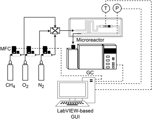
A silicon-glass microreactor was fabricated using photolithography, deep reactive ion etching and anodic bonding. The reaction channel was 0.42 and 2 mm deep and wide, respectively, and contained the catalyst for the reaction. The catalyst was held in place in the reaction zone by a retainer, present at the end of the reaction zone. The microreactor could be employed for the reaction up to a maximum temperature of 400 °C. For temperature monitoring within the catalyst bed, the reactor had six dead-end slots for inserting K-type thermocouples. Further details are available in our previous work.35 A schematic of the experimental set-up is shown in Fig. 2. The composition of the inlet stream was made up of 5% methane in helium, oxygen and nitrogen as the internal standard. The pressure was monitored with pressure sensors (Honeywell, 40PC, 100 psig). To maintain a constant desired reactor outlet pressure, a pressure controller (Brooks, 5866) was placed after the microreactor. The mole fractions of methane, oxygen and carbon dioxide were measured with an online gas chromatograph (Agilent, 7890A), equipped with a pneumatic sampling valve, 0.25 mL sampling loop, GS-Carbon PLOT (Agilent), HP-PLOT molecular sieve (Agilent) columns and thermal conductivity detector. Hardware automation was achieved by integration of all the hardware components by means of Python-LabVIEW. In the automated procedure, the gas chromatograph automatically saved the measured data in an Excel file. A Python code was used to access this file and save the measured data in another Excel file called the record file. The experimental conditions were also saved in the record file. The record file was updated after each experiment and the updated file was used as the data source for the parameter estimation algorithm. Using the timed loop in LabVIEW, the duration for each experiment, which was composed of the reaction time and the analysis time in the gas chromatograph, was set at 20 minutes. The solid lines in Fig. 2 show the gas flow paths. The dashed lines represent the communication of control/measured signals of the mass flow controllers, the temperature controller, the pressure controller and the gas chromatograph. The control signals are the signals sent from the LabVIEW-based graphical user interface (GUI) to the control devices. The measured signals are the signals read from different sensors, which are displayed on the GUI. Further details on the development of the automated experimental platform are available in ref. 35.
 |
| | Fig. 2 Schematic of the methane complete catalytic oxidation system. MFC: mass flow controller, T: temperature control, P: pressure control and GC: gas chromatograph. The solid lines indicate gas flow paths, and the dashed lines indicate control/measured signals. | |
3.2 Mass and heat transfer resistances
The reaction system was assumed to be unaffected by mass transfer resistances, which was verified by computing the Mear's criterion and the Weisz–Prater number55 for external and internal mass transfer resistances, respectively. The most severe experimental conditions of high temperature and high reactant concentrations were used for the Mear's criterion calculation and a value of 0.026 (which is less than 0.15) was obtained, suggesting that the external mass transfer limitation can be ignored. For the internal mass transfer resistance calculation, the Weisz–Prater criterion evaluation resulted in a value of 0.13, (which was less than 1), suggesting that the internal mass transfer resistance can be neglected. More details about these calculations are provided in our previous work.35 The criterion for isothermal conditions within the catalyst particles was also satisfied, based on the condition that the observed rate of reaction must not differ more than 5% from the actual reaction rate within the catalyst particle at constant temperature. According to the Mear's criterion for external heat transfer resistance, a value <0.15 implies that the external heat transfer limitation could be neglected. The value obtained was 0.3, hence there was a need to estimate the catalyst surface temperature (Ts) from the measured temperature (Tm), assumed to be the same as the bulk fluid temperature. A correlation based on the preliminary data was used to develop a relationship between Tm and Ts, and shown as a linear relationship in Fig. 3. Detailed discussion on external heat transfer limitations and on the justification to use a linear relationship to correlate the catalyst surface temperature and measured reactor temperature is provided in the supporting information of our previous work.35 The linear relationship shown in Fig. 3 was employed within LabVIEW for regulating the temperature controller by reading the measured temperature rather than the catalyst surface temperature. However, the catalyst surface temperature was used for the kinetic studies. Axial dispersion was assumed to be negligible in the packed bed reactor based on the calculated aspect ratio. More information about the experimental set-up and reaction system can be found in our previous work.35
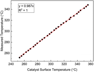 |
| | Fig. 3 Calculated catalyst particle surface temperature against measured temperature in the microreactor for catalytic methane combustion. | |
3.3 Reactor model
With the assumptions stated above, the micro-packed bed reactor was modelled as an isothermal plug flow reactor (PFR)35 using the following set of ordinary differential equations (ODEs)| | 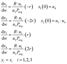 | (13) |
In eqn (13), the state variables x1, x2, x3 and x4 represent the mole fractions [mol mol−1] of methane, oxygen, carbon dioxide and water, respectively. The control variables in the process include the reaction temperature [°C], flow rate of the feed [Nml min−1], oxygen to methane mole ratio in the feed [mol mol−1] and inlet methane mole fraction [mol mol−1], which are respectively denoted as u1, u2, u3 and u4. These controls form the design vector φ, which defines the conditions of an experiment. The design vector φ is bounded within the experimental design domain shown in Table 1. In eqn (13), R [J mol−1 K−1] is the universal gas constant, r [mol g−1 min−1] represents the reaction rate according to a postulated kinetic model, w [g] is the catalyst mass along the packed bed reactor (the domain of independent variable) and Pavg [bar] is the average pressure along the packed bed reactor, which was estimated using a pressure drop model.35
Table 1 Range of control variables. Temperature is measured in the reactor, while all the other variables are at the reactor inlet
| Control variable |
Temperature [°C] |
Mass flow rate [Nml min−1] |
Oxygen to methane mole ratio [mol mol−1] |
Methane mole fraction [mol mol−1] |
| Range |
250–350 |
20–30 |
2–4 |
0.005–0.025 |
The steady state mole fractions of methane, oxygen and carbon dioxide at the reactor outlet, measured across the performed experiments, formed the output data set Y. The random error in observations was computed from repeated measurements using the method of pooled standard deviation,35 and the covariance matrix of measurement error was estimated as
| |  | (14) |
The diagonal entries of the matrix
Σy are the variances of random measurement error associated with measurement of methane, oxygen, and carbon dioxide mole fractions, respectively.
3.4 Candidate kinetic models
Based on the results of a preliminary screening of kinetic models, which is discussed in ref. 35, three candidate kinetic models were considered as the potential models to describe the methane complete oxidation reaction. The reaction mechanisms governing the models and the respective rate laws are provided in Table 2.
Table 2 Candidate kinetic models considered in this work
| Model |
Description |
Rate law |
| Model 1 |
Power law model |
r
CH4 = k1PCH4 |
| Model 2 |
Langmuir Hinshelwood (LH) mechanism (surface reaction between adsorbed methane and dissociatively chemisorbed oxygen56,57) |

|
| Model 3 |
Mars van Krevelen (MVK) mechanism (slow desorption of the reaction products56,57) |

|
3.5 Reparameterisation of kinetic parameters
In order to minimise the correlation between kinetic parameters and to scale all the parameters to comparable magnitudes, the Arrhenius (eqn (15)) and van't Hoff (eqn (16)) equations used in the kinetic models were reparameterised58,59 as| |  | (15) |
| |  | (16) |
In eqn (15), k(T) is the reaction rate constant at temperature T, Ea is the activation energy and Tref = 320 °C is the reference temperature. Similarly, in eqn (16), K(T) is the equilibrium constant of adsorption at temperature T and ΔH is the enthalpy of adsorption. The actual parameters, units, and their reparameterised form for each of the candidate kinetic models are listed in Table 3. Instead of estimating the actual kinetic model parameters, the reparameterised parameters were estimated in the parameter estimation step.
Table 3 Actual parameters, units, and their reparameterised form for each of the kinetic models
| Model |
Actual parameter |
Unit |
Reparameterised form |
| Model 1 |
k
1
|
mol bar−1 g−1 min−1 |
θ
1 = −log![[thin space (1/6-em)]](https://www.rsc.org/images/entities/char_2009.gif) k1(Tref) k1(Tref) |
|
E
a1
|
J mol−1 |

|
| Model 2 |
k
r
|
mol g−1 min−1 |
θ
1 = −log![[thin space (1/6-em)]](https://www.rsc.org/images/entities/char_2009.gif) kr(Tref) kr(Tref) |
|
E
ar
|
J mol−1 |

|
|
K
O2
|
bar−1 |
θ
3 = log![[thin space (1/6-em)]](https://www.rsc.org/images/entities/char_2009.gif) KO2(Tref) KO2(Tref) |
| ΔHO2 |
J mol−1 |

|
|
K
CH4
|
bar−1 |
θ
5 = log![[thin space (1/6-em)]](https://www.rsc.org/images/entities/char_2009.gif) KCH4(Tref) KCH4(Tref) |
| ΔHCH4 |
J mol−1 |

|
| Model 3 |
k
1
|
mol bar−1 g−1 min−1 |
θ
1 = −log![[thin space (1/6-em)]](https://www.rsc.org/images/entities/char_2009.gif) k1(Tref) k1(Tref) |
|
E
a1
|
J mol−1 |

|
|
k
2
|
mol bar−1 g−1 min−1 |
θ
3 = −log![[thin space (1/6-em)]](https://www.rsc.org/images/entities/char_2009.gif) k2(Tref) k2(Tref) |
|
E
a2
|
J mol−1 |

|
|
k
3
|
mol g−1 min−1 |
θ
5 = −log![[thin space (1/6-em)]](https://www.rsc.org/images/entities/char_2009.gif) k3(Tref) k3(Tref) |
|
E
a3
|
J mol−1 |

|
3.6 Computational resources
All the computational procedures used in this work were performed on a 64-bit Windows machine with Intel® Core™ i7-8550U CPU, 2.00 GHz processor and 8.00 GB RAM. The Python model identification framework was built in Python version 3.7.4. In the Python framework, the pyDOE2 package60 was used for the design of preliminary factorial experiments. The candidate kinetic models described by a set of ODEs were written as Python functions. Solution of ODEs and simulation of the models including the computation of sensitivity functions were carried out using the odeint function within the Scipy61 package (scipy.integrate.odeint) with the lsoda62 integrator. Parameter estimation was carried out in Pyomo using the Interior Point OPTimizer (IPOPT) solver.63 The MBDoE problems were solved using the Sequential Least SQuares Programming (SLSQP)64 solver in the minimize function in the Scipy.optimize class.
4 Results and discussion
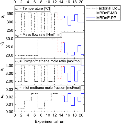
Given the candidate kinetic models as input, the autonomous platform was able to perform unmanned experiments until the appropriate kinetic model of methane complete oxidation was identified. The experimental settings used by the platform in order to achieve this task comprised a campaign of factorial experiments (experiments 1–12) designed using the two-level fractional factorial DoE method, MBDoE-MD experiments (experiments 13 and 14) and MBDoe-PP experiments (experiments 15–20). The experimental conditions of these campaigns are shown in Fig. 4. The full set of experimental data is provided in the ESI.†
 |
| | Fig. 4 Experimental conditions in the factorial, MBDoE-MD and MBDoE-PP campaign of experiments, used by the autonomous platform for identification of an appropriate kinetic model for methane oxidation. | |
4.1 Preliminary factorial experiments and first parameter estimation
As shown in Fig. 4, the factorial experiments consisted of two 2-level fractional factorial designs; one in which the ranges of input variables specified in Table 1 were used as levels and the other where the same ranges were used as levels except for the inlet methane concentration for which a lower level of 0.015 was used. The experiments which were common in both 2-level fractional factorial designs were performed only once. The autonomous operation of the platform did not start until the factorial experiments were finished. The output data from the factorial experiments were used for the first online parameter estimation. The results of the first online parameter estimation are given in Table 4. It can be seen from the table that at the end of factorial experiments, i.e., at the end of experiment 12, model 1 (power law model) showed poor data compatibility and failed the chi-square goodness of fit test. Meanwhile, both model 2 LH and model 3 MVK passed the chi-square goodness of fit test, however with almost the same chi-square values. This resulted in almost equal probabilities (≈50%) for both models. Immediately the autonomous decision module and the model-based design of experiments module of the platform were triggered to design new MBDoE experiments for discriminating between model 2 and model 3.
Table 4 Parameter estimation results showing chi-square and probability of model adequacy for candidate models at the end of the factorial campaign of experiments, i.e., at the end of experiment 12. The values in bold indicate a failure of the chi-square test, which happens when the computed value of chi-square becomes greater than the reference chi-square value
| Model |
Adequacy χ2/χ2ref |
Probability of model adequacy (%) |
| Model 1 |
63.34/48.60
|
0.11 |
| Model 2 |
23.63/43.77 |
51.64 |
| Model 3 |
24.75/43.77 |
48.25 |
4.2 MBDoE assisted experiments and decisions made by the autonomous decision module
The parameter estimation results showing the chi-square values and the probability values for all the candidate models at the end of MBDoE-MD experiments are shown in Table 5. The same results can be read from the adequacy graph provided in Fig. 5. The MBDoE-MD campaign of experiments started from experiment 13 and continued until the chi-square criterion (χ2 < χ2ref) and the probability criterion (Prj > 90%) confirmed a satisfactory discrimination between the models. This was achieved at the end of experiment 14, when model 3 (MVK model) was found to be the most appropriate kinetic model, which agrees with the results of similar studies in the literature.57 It is interesting to see from Fig. 4 that high temperature (T > 300 °C), high oxygen to methane mole ratio (≈4 mol mol−1) and high inlet methane mole fraction (≈0.02 mol mol−1) resulted in the highest discriminating power between model 2 and model 3 (experiment 14). This agrees with the literature suggesting that high methane concentration and high temperature promote the rate of surface reduction and surface re-oxidation steps in the MVK mechanism, which is the striking difference between the LH and MVK mechanisms i.e., between model 2 and model 3.56,57 It can be seen from both Table 5 and Fig. 5 that at the end of experiment 14, only model 3 passed the chi-square test with a probability value of 93%. This automatically moved switch S1 to an open position and S2 to a closed position (see Fig. 1), by selecting model 3 as the appropriate model. At this stage, except parameters 3 and 4 (underlined in Table 6), all the parameters of model 3 were estimated precisely according to Student's t-test. The statistical precision of parameter estimates of model 3 at the end of the MBDoE-MD campaign of experiments can be also read from the graph of 95% confidence intervals and t-values of parameter estimates, shown in Fig. 6. The failure of the t-test for parameters 3 and 4 triggered the MBDoE-PP methods to design new experiments for improving the precision of parameter estimates. The MBDoE-PP experiments started from experiment 15 and continued until all the parameters of model 3 passed the t-test. This was achieved at the end of experiment 20. It can be seen from Table 7 and Fig. 6 that at the end of experiment 20, all the parameters of model 3 passed the t-test and the 95% confidence intervals for all parameter estimates have become narrow positive sets.
Table 5 Parameter estimation results showing chi-square and probability of model adequacy for candidate models at the end of the MBDoE-MD campaign of experiments, i.e., at the end of experiment 14. The values in bold indicate a failure of the chi-square test, which happens when the computed value of chi-square becomes greater than the reference chi-square value
| Model |
Adequacy χ2/χ2ref |
Probability of model adequacy (%) |
| Model 1 |
142.96/55.76
|
0 |
| Model 2 |
54.80/50.99
|
6.83 |
| Model 3 |
39.52/50.997 |
93.17 |
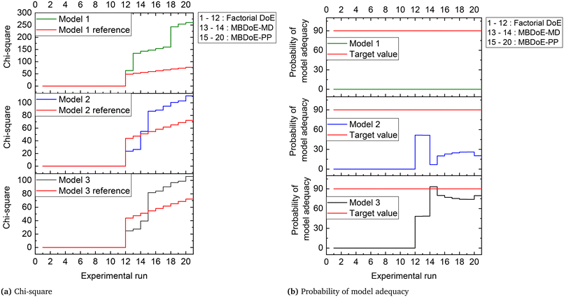 |
| | Fig. 5 (a) Chi-square value and (b) probability of model adequacy computed for candidate models in the experimental runs in the campaigns indicated. | |
Table 6 Parameter estimation results showing the estimated values, 95% confidence interval (C.I) and t-values of parameters of model 3 at the end of the MBDoE-MD experimental campaign. Note that the value of tref is 1.68
| Parameter |
Estimate ±95% C.I |
t-Value |
|
θ
1
|
5.99 ± 0.39 |
15.14 |
|
θ
2
|
6.93 ± 3.59 |
1.93 |
|
θ
3
|
4.00 ± 2.54 |
![[1 with combining low line]](https://www.rsc.org/images/entities/char_0031_0332.gif) . .![[5 with combining low line]](https://www.rsc.org/images/entities/char_0035_0332.gif) ![[7 with combining low line]](https://www.rsc.org/images/entities/char_0037_0332.gif) |
|
θ
4
|
9.31 ± 20.05 |
![[0 with combining low line]](https://www.rsc.org/images/entities/char_0030_0332.gif) . .![[4 with combining low line]](https://www.rsc.org/images/entities/char_0034_0332.gif) ![[6 with combining low line]](https://www.rsc.org/images/entities/char_0036_0332.gif) |
|
θ
5
|
10.48 ± 0.20 |
51.26 |
|
θ
6
|
7.04 ± 1.79 |
3.94 |
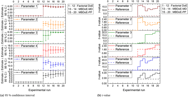 |
| | Fig. 6 (a) Confidence interval (95%) and (b) t-values for parameter estimates of model 3, updated in the experimental runs in the campaigns indicated. | |
Table 7 Parameter estimation results showing the estimated values, 95% confidence interval (C.I) and t-values of parameters of model 3 at the end of the MBDoE-PP experimental campaign. Note that the value of tref is 1.67
| Parameter |
Estimate ±95% C.I |
t-Value |
|
θ
1
|
5.77 ± 0.36 |
15.91 |
|
θ
2
|
6.72 ± 3.81 |
1.76 |
|
θ
3
|
5.87 ± 0.27 |
21.94 |
|
θ
4
|
9.51 ± 3.62 |
2.62 |
|
θ
5
|
10.17 ± 0.18 |
57.38 |
|
θ
6
|
7.98 ± 2.12 |
3.76 |
Although parameters 3 and 4 initially appeared to be the critical parameters, which were not estimated precisely at the end of the MBDoE-MD campaign, further experimentation proved that parameters 2 and 4 were the critical parameters. The 95% confidence ellipses showing the uncertainty regions of parameter pairs (2 and 4) and (3 and 4) are shown in Fig. 7. A careful evaluation of the confidence ellipses in Fig. 7 suggests that experiment 15 (high temperature 327 °C and high oxygen to methane mole ratio 4) significantly reduced the uncertainty region of parameter 4, which is the activation energy of the surface reduction step in model 3. Meanwhile, experiment 20 resulted in reducing the size of the uncertainty region of parameter 2, which is the activation energy of the surface oxidation step of model 3. Another interesting result regarding the correlation between parameters of model 3 at the end of the factorial, MBDoE-MD and MBDoE-PP experimental campaigns is shown in Fig. 8. It can be observed from the figure that none of the parameters had perfect correlation or anti-correlation at the end of the MBDoE-PP campaign. Moreover, the correlation between the parameters was relatively reduced in the course of experimentation, suggesting good validity of the t-test.
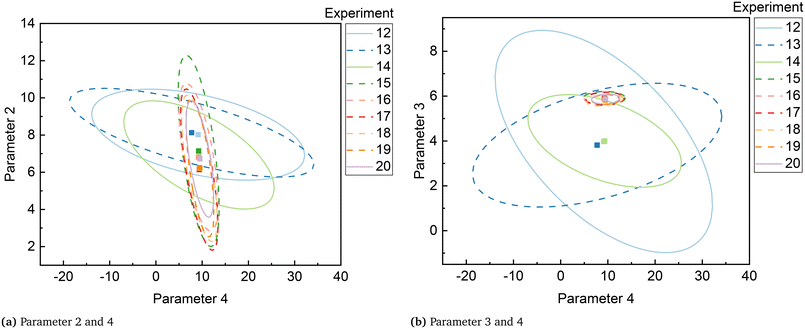 |
| | Fig. 7 Confidence ellipses for critical parameter pairs of model 3 (a) parameter 2 and 4 and (b) parameter 3 and 4, at the end of the experiment indicated. | |
 |
| | Fig. 8 Correlation matrices of model 3 at the end of the (a) factorial DoE, (b) MBDoE-MD and (c) MBDoE-PP experimental campaigns. | |
The values of reaction rate constant (at the reference temperature), pre-exponential factor and activation energy for different steps of model 3 were obtained from the final parameter estimates of model 3. These values are provided in Table 8. A comparison of the reaction rate constants at the reference temperature (320 °C) indicates that the slowest step in the mechanism is the desorption of products, which agrees with the assumptions of model 3. In addition, the values of activation energies for surface oxidation and desorption of products, obtained in this study (67.2 ± 38.1, 79.8 ± 21.2 kJ mol−1) are comparable (considering the uncertainty limit) to those (51.5, 108.5 kJ mol−1) obtained for the oxidation of methane over commercial 0.5% Pd on γ-Al2O3.57 However, the activation energy for the surface reduction step obtained in this work (95.1 ± 36.2 kJ mol−1) is higher than that (16.8 kJ mol−1) reported in the literature.57
Table 8 The values of rate constant, pre-exponential factor and activation energies for different steps of model 3
| Reaction step |
Rate constant at the reference temperature Tref |
Pre-exponential factor |
Activation energy kJ mol−1 |
| Surface oxidation |
k
1 = 3.12 × 10⁻³ mol bar−1 g−1 min−1 |
2.58 × 10³ mol bar−1 g−1 min−1 |
E
a1 = 67.2 |
| Surface reduction |
k
2 = 2.82 × 10⁻³ mol bar−1 g−1 min−1 |
6.69 × 10⁵ mol bar−1 g−1 min−1 |
E
a2 = 95.1 |
| Desorption of products |
k
3 = 3.83 × 10⁻⁵ mol g−1 min−1 |
4.08 × 10² mol g−1 min−1 |
E
a3 = 79.8 |
4.3 Retrospective analysis of models
It should be noted that at the end of the MBDoE-PP experimental campaign, both model 2 and model 3 failed the chi-square goodness of fit test. This is clearly shown in the adequacy graph of Fig. 5. In addition, the computed chi-square values were very close for both the models, indicating their similar behaviour. This led to the retrospective analysis of the models using prediction density plots as well as residual plots. The prediction density plots for models 2 and 3 were created based on the methods discussed in section 2.6. The joint prediction density plots of models 2 and 3 using the final parameter estimates were created for each experimental condition and for each of the output variables. This analysis aimed to better study the degree of discrimination between the two models.
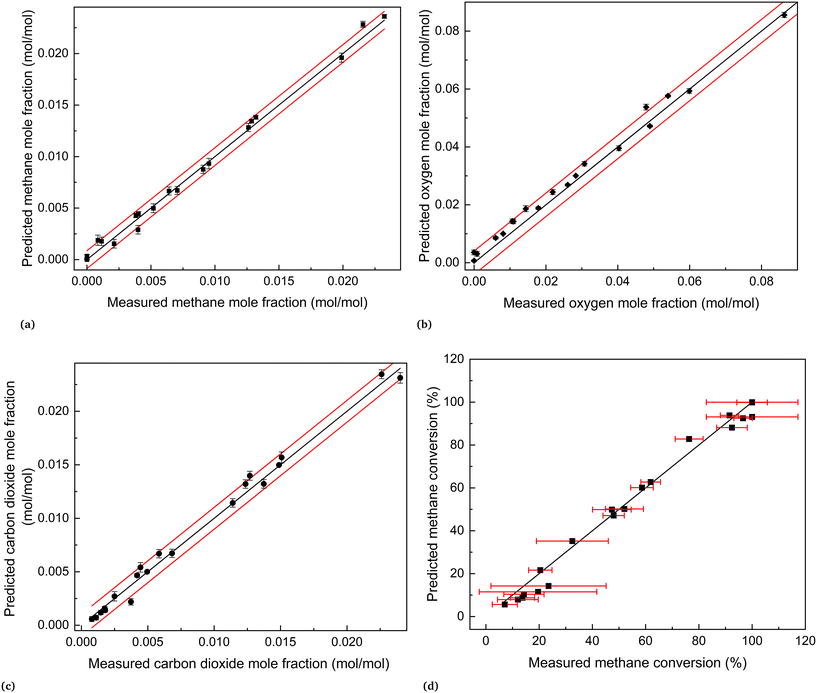
The joint prediction density plots of the models along with the experimental observation within its error bound suggested that it is very difficult to discriminate between models 2 and 3 using the observables. In most of the cases, the degree of discrimination was found negligible compared to the magnitude of random error in observations. The full set of prediction density plots is provided in the ESI.† The case where the degree of discrimination between the models is at least as significant as the error in observation was obtained for experiment 14. In experiment 14, the difference between the model predictions relative to the respective uncertainty limits is significant for methane and carbon dioxide. This is shown in the joint prediction density plots in Fig. 9. In the figure, the difference between the means of the prediction distributions of methane and carbon dioxide and also the difference between different observations of the two distributions (panels (a) and (c) of Fig. 9) are greater than the standard deviation (half the error bound in the figure) of measurement error of methane and carbon dioxide. The result suggests that experiment 14 provided the only conditions where the models are significantly distinguishable. This aligns with the results suggested by the MBDoE-MD optimization, which also suggested that experiment 14 provided the optimal conditions to discriminate between the two models. The prediction density plots also indicate that compared to model 2, the observed values within their error bounds are less contradicted by model 3. The residual plots of models 2 and 3, showing the magnitude of prediction error (based on the final parameter estimates) for each experimental condition and for each of the output variables, were also studied to compare with the results of prediction density plots. From the prediction density plots, the prediction error or residuals can be computed as the difference between the means of the distribution and the corresponding observed values. The residuals computed in this manner from the density plots are in alignment with the residuals shown in Fig. 10, which are computed as the difference between model predictions and the observed values. The residual plots also suggested that both models 2 and 3 had large residuals at experiments 5 and 12. A comparison of model predicted and experimental values for model 3 at the end of the experimental campaign is provided in Fig. 11 in the form of parity plots. As shown in the figure, model 3 provides close predictions to the experimental data. Another interesting fact drawn from the figure is the narrow uncertainty intervals of predictions of the model evaluated from Vŷ(·) computed using eqn (11). Compared to the uncertainty in measurements, the negligibly small uncertainty intervals of model predictions are the result of the precise estimation of model parameters, which are the main source of uncertainty in model predictions. The details about computation of error bounds in panel (d) of Fig. 11, which shows the parity plot of model 3 in terms of methane conversion, are provided in the ESI.†
 |
| | Fig. 9 Prediction density plots showing uncertainty in predictions of models 2 and 3 at experiment 14 (reaction temperature = 325.9 °C, mass flow rate = 27.7 Nml min−1, oxygen/methane mole ratio = 3.9 mol mol−1, inlet methane concentration = 0.022 mol mol−1) for (a) methane, (b) oxygen and (c) carbon dioxide. The observed value is shown as a point with the error bar (± standard deviation). | |
 |
| | Fig. 10 Residual plots for models 2 and 3 (in terms of (a) methane, (b) oxygen and (c) carbon dioxide) based on the final parameter estimates. | |
 |
| | Fig. 11 Parity plots of model 3 at the end of the experimental campaign, i.e., at the end of experiment 20: (a) methane, (b) oxygen and (c)carbon dioxide. In (a)–(c), the black line represents the perfect agreement between the measured and the predicted values, and the two red lines represent the measurement error (±2 × standard deviation). The error bars were calculated as ±2 × standard deviation of predictions. Panel (d) shows a comparison of experimental and predicted values of methane conversion. In (d), the black line represents the perfect agreement between the measured and the predicted conversions, computed from the corresponding concentration values. The red error bars represent the error bounds (±2 × standard deviation) of methane conversion, computed from error in measured concentration values. | |
4.4 Algorithm performance
The computational time for parameter estimation problems was close to 7 CPU seconds, whereas the solution of MBDoE problems took approximately 30 CPU seconds. Our implementation is available at https://github.com/UCL/Methane_oxidation.
5 Conclusions
An autonomous microreactor platform powered by optimal experimental design methods and data analysis was developed and successfully applied for kinetic model identification. The computational framework of the platform was developed in the Python programming language and was integrated to a LabVIEW program controlling the microreactor system. A new Pyomo-based parameter estimation module was employed in the framework for the efficient solution of online parameter estimation problems. In addition, a probability criterion derived from the chi-square goodness of fit test was defined for online selection of appropriate models. The platform was successfully demonstrated on identifying an appropriate kinetic model along with precise estimation of its parameters for methane complete catalytic oxidation on a Pd/Al2O3 catalyst. A total of 20 automated experiments were completed in two days for this purpose. Among the different kinetic models tested (Power law, Langmuir Hinshelwood and Mars van Krevelen), the Mars van Krevelen model was found to be the most appropriate, which agrees with similar studies reported in the literature. The activation energies for the surface oxidation, surface reduction, and product desorption steps of the Mars van Krevelen model were estimated to be 67.2, 95.1 and 79.8 kJ mol−1, respectively. Prediction density plots were employed as retrospective data analysis tools that are useful to review and reassess the decisions taken by the platform over time. In general, the prediction density plots together with experimental data provide insight about the uncertainty as well as adequacy of models in representing the data and their assumed distribution. The joint prediction density plots are also valuable tools to better understand the degree of discrimination between the competing models.
Glossary
Acronyms
| CASP | Computer aided synthesis planning |
| DAEs | Differential and algebraic equations |
| DoE | Design of experiments |
| FIM | Fisher information matrix |
| GC | Gas chromatograph |
| GSD | Generalized subset design |
| GUI | Graphical user interface |
| IPOPT | Interior Point OPTimizer |
| LH | Langmuir Hinshelwood |
| MBDoE | Model-based design of experiments |
| MBDoE-MD | MBDoE for model discrimination |
| MBDoE-PP | MBDoE for improving parameter precision |
| MVK | Mars van Krevelen |
| NLP | Nonlinear programming |
| ODE | Ordinary differential equation |
| PFR | Plug flow reactor |
| Pyomo | Python optimization modeling objects |
| RMG | Reaction mechanism generator |
| RMS | Reaction modelling suite |
| SLSQP | Sequential Least SQuares Programming |
Latin symbols
| det | Determinant of a matrix |
|
E
a
| Activation energy |
|
k
| Reaction rate constant |
|
n
| Total number of samples |
|
N
| Total number of observations |
![[scr N, script letter N]](https://www.rsc.org/images/entities/char_e52d.gif) (·, ·) (·, ·) | Normal distribution with specified mean and variance |
|
N
exp
| Number of performed experiments |
|
N
θ
| Number of model parameters |
|
N
y
| Number of response variables |
|
p(·) | Probability density function |
|
T
ij
(·) | Objective function to discriminate between models i and j |
Greek symbols
|
α
| Significance level |
|
ε
| Measurement error |
|
θ
i
|
i-th model parameter |
![[small straight theta, Greek, circumflex]](https://www.rsc.org/images/entities/b_char_e12d.gif) i
i
| Estimate of i-th model parameter |
|
χ
2
| Sum of squared residuals |
|
ψ(·) | Objective function of the MBDoE-PP problem |
Vectors and matrices
|
C
θ
| [Nθ × Nθ] parameter correlation matrix |
|
f(·) | Vector of functions representing the state equation |
|
h(·) | Vector of functions representing the output equation |
|
H
θ
| [Nθ × Nθ] Fisher information matrix |
|
T
sp
| List of full set of sampling times (over all experiments) |
|
u(·) | Vector [Nu × 1] of inputs or control variables |
|
U
| List of full set of inputs (over all experiments) |
|
V
ŷ
| [Ny × Ny] covariance matrix of model predictions |
|
V
θ
| [Nθ × Nθ] parameter covariance matrix |
|
x(·) | Vector of state variables |
![[x with combining circumflex]](https://www.rsc.org/images/entities/b_char_0078_0302.gif) (·) (·) | Vector of first derivatives of state variables |
|
y(·) | Vector [Ny × 1] of outputs or response variables |
|
ŷ(·) | Vector of model predictions of the output variables |
|
Y
| List of full set of outputs (over all experiments) |
|
θ
| Vector [Nθ × 1] of model parameters |
|
Σy
| Covariance matrix [Ny × Ny] of measurement error |
|
φ
| Design vector |
Conflicts of interest
There are no conflicts to declare.
Acknowledgements
A. Pankajakshan thanks the Department of Chemical Engineering, University College London for his PhD studentship and S. G. Bawa thanks the Petroleum Technology Development Fund for his PhD studentship (PTDF/ED/PHD/BSG/1362/18). We thank Johnson Matthey for providing the catalyst.
References
- M. B. Plutschack, B. Pieber, K. Gilmore and P. H. Seeberger, Chem. Rev., 2017, 117, 11796–11893 CrossRef CAS PubMed.
- A. Manz, N. Graber and H. Á. Widmer, Sens. Actuators, B, 1990, 1, 244–248 CrossRef CAS.
- K. F. Jensen, Chem. Eng. Sci., 2001, 56, 293–303 CrossRef CAS.
- S. Katare, Comput.-Aided Chem. Eng., 2003, 14, 701–706 CAS.
- C. W. Gao, J. W. Allen, W. H. Green and R. H. West, Comput. Phys. Commun., 2016, 203, 212–225 CrossRef CAS.
- M. Liu, A. Grinberg Dana, M. S. Johnson, M. J. Goldman, A. Jocher, A. M. Payne, C. A. Grambow, K. Han, N. W. Yee and E. J. Mazeau,
et al.
, J. Chem. Inf. Model., 2021, 61, 2686–2696 CrossRef CAS PubMed.
- N. M. Vandewiele, K. M. Van Geem, M.-F. Reyniers and G. B. Marin, Chem. Eng. J., 2012, 207, 526–538 CrossRef.
- P. S. Mendes, S. Siradze, L. Pirro and J. W. Thybaut, React. Chem. Eng., 2022, 7, 142–155 RSC.
- C. W. Coley, N. S. Eyke and K. F. Jensen, Angew. Chem., Int. Ed., 2020, 59, 22858–22893 CrossRef CAS PubMed.
- C. W. Coley, N. S. Eyke and K. F. Jensen, Angew. Chem., Int. Ed., 2020, 59, 23414–23436 CrossRef CAS PubMed.
- C. W. Coley, D. A. Thomas III, J. A. Lummiss, J. N. Jaworski, C. P. Breen, V. Schultz, T. Hart, J. S. Fishman, L. Rogers and H. Gao,
et al.
, Science, 2019, 365, eaax1566 CrossRef CAS PubMed.
- A. Echtermeyer, Y. Amar, J. Zakrzewski and A. Lapkin, Beilstein J. Org. Chem., 2017, 13, 150–163 CrossRef CAS PubMed.
- A. M. Schweidtmann, A. D. Clayton, N. Holmes, E. Bradford, R. A. Bourne and A. A. Lapkin, Chem. Eng. J., 2018, 352, 277–282 CrossRef CAS.
- C. A. Hone, N. Holmes, G. R. Akien, R. A. Bourne and F. L. Muller, React. Chem. Eng., 2017, 2, 103–108 RSC.
- J. S. Moore and K. F. Jensen, Org. Process Res. Dev., 2012, 16, 1409–1415 CrossRef CAS.
- B. J. Reizman, Y.-M. Wang, S. L. Buchwald and K. F. Jensen, React. Chem. Eng., 2016, 1, 658–666 RSC.
-
R. A. Fisher, The design of experiments, Oliver & Boyd, Edinburgh, 1935 Search PubMed.
- G. E. Box and H. Lucas, Biometrika, 1959, 46, 77–90 CrossRef.
-
G. E. Box and N. R. Draper, Empirical model-building and response surfaces, John Wiley & Sons, Blackwell, 1987 Search PubMed.
- S. Asprey and S. Macchietto, Comput. Chem. Eng., 2000, 24, 1261–1267 CrossRef CAS.
- G. Franceschini and S. Macchietto, Chem. Eng. Sci., 2008, 63, 4846–4872 CrossRef CAS.
- J. P. McMullen and K. F. Jensen, Org. Process Res. Dev., 2011, 15, 398–407 CrossRef CAS.
- B. J. Reizman and K. F. Jensen, Org. Process Res. Dev., 2012, 16, 1770–1782 CrossRef CAS.
- S. D. Schaber, S. C. Born, K. F. Jensen and P. I. Barton, Org. Process Res. Dev., 2014, 18, 1461–1467 CrossRef CAS.
- C. Waldron, A. Pankajakshan, M. Quaglio, E. Cao, F. Galvanin and A. Gavriilidis, React. Chem. Eng., 2019, 4, 1623–1636 RSC.
- C. Waldron, A. Pankajakshan, M. Quaglio, E. Cao, F. Galvanin and A. Gavriilidis, React. Chem. Eng., 2020, 5, 112–123 RSC.
- M. Quaglio, C. Waldron, A. Pankajakshan, E. Cao, A. Gavriilidis, E. S. Fraga and F. Galvanin, Comput. Chem. Eng., 2019, 124, 270–284 CrossRef CAS.
- C. Waldron, A. Pankajakshan, M. Quaglio, E. Cao, F. Galvanin and A. Gavriilidis, Ind. Eng. Chem. Res., 2019, 58, 22165–22177 CrossRef CAS.
- C. J. Taylor, H. Seki, F. M. Dannheim, M. J. Willis, G. Clemens, B. A. Taylor, T. W. Chamberlain and R. A. Bourne, React. Chem. Eng., 2021, 6, 1404–1411 RSC.
- M. N. Cruz Bournazou, T. Barz, D. Nickel, D. C. Lopez Cárdenas, F. Glauche, A. Knepper and P. Neubauer, Biotechnol. Bioeng., 2017, 114, 610–619 CrossRef CAS PubMed.
- W. E. Hart, J.-P. Watson and D. L. Woodruff, Math. Program. Comput., 2011, 3, 219–260 CrossRef.
-
M. L. Bynum, G. A. Hackebeil, W. E. Hart, C. D. Laird, B. L. Nicholson, J. D. Siirola, J.-P. Watson and D. L. Woodruff, et al., Pyomo-optimization modeling in Python, Springer, Cham, Switzerland, 2021 Search PubMed.
- B. Nicholson, J. D. Siirola, J.-P. Watson, V. M. Zavala and L. T. Biegler, Math. Program. Comput., 2018, 10, 187–223 CrossRef.
- I. Surowiec, L. Vikstrom, G. Hector, E. Johansson, C. Vikstrom and J. Trygg, Anal. Chem., 2017, 89, 6491–6497 CrossRef CAS PubMed.
- S. G. Bawa, A. Pankajakshan, C. Waldron, E. Cao, F. Galvanin and A. Gavriilidis, Chem.: Methods, 2023, 3, e202200049 CAS.
- R. A. Fisher, Philos. Trans. R. Soc., A, 1922, 222, 309–368 Search PubMed.
-
Y. Bard, Nonlinear parameter estimation, Academic Press, New York, 1974 Search PubMed.
- A. B. Singer, J. W. Taylor, P. I. Barton and W. H. Green, J. Phys. Chem. A, 2006, 110, 971–976 CrossRef CAS PubMed.
- R. Ramachandran and P. I. Barton, Chem. Eng. Sci., 2010, 65, 4884–4893 CrossRef CAS.
-
H. G. Bock, S. Körkel and J. P. Schlöder, Parameter Estimation and Optimum Experimental Design for Differential Equation Models, in Model Based Parameter Estimation: Theory and Applications, ed. H. G. Bock, T. Carraro, W. Jäger, S. Körkel, R. Rannacher and J. P. Schlöder, Springer, Berlin, Heidelberg, 2013, pp. 1–30 Search PubMed.
-
L. T. Biegler, Nonlinear programming: concepts, algorithms, and applications to chemical processes, SIAM, 2010 Search PubMed.
-
R. A. Fisher, Statistical methods for research workers, Oliver & Boyd, Edinburgh, 11th edn, 1950 Search PubMed.
- J. Neyman and E. S. Pearson, Philos. Trans. R. Soc., A, 1933, 231, 289–337 Search PubMed.
- K. Pearson, Philos. Mag., 1900, 50, 157–175 Search PubMed.
- Student, Biometrika, 1908, 6, 1–25 CrossRef.
-
A. Saltelli, S. Tarantola, F. Campolongo and M. Ratto, Sensitivity analysis in practice: a guide to assessing scientific models, Wiley, New York, 2004 Search PubMed.
-
A. Saltelli, M. Ratto, T. Andres, F. Campolongo, J. Cariboni, D. Gatelli, M. Saisana and S. Tarantola, Global sensitivity analysis: the primer, John Wiley & Sons, Chichester, West Sussex, 2008 Search PubMed.
- I. Sokolović, M. Reticcioli, M. Čalkovský, M. Wagner, M. Schmid, C. Franchini, U. Diebold and M. Setvín, Proc. Natl. Acad. Sci. U. S. A., 2020, 117, 14827–14837 CrossRef PubMed.
- M. Schwaab, F. M. Silva, C. A. Queipo, A. G. Barreto Jr, M. Nele and J. C. Pinto, Chem. Eng. Sci., 2006, 61, 5791–5806 CrossRef CAS.
- G. B. Ferraris, P. Forzatti, G. Emig and H. Hofmann, Chem. Eng. Sci., 1984, 39, 81–85 CrossRef.
-
E. Walter and L. Pronzato, Identification of parametric models from experimental data, Springer Verlag, New York, 1997 Search PubMed.
- C. J. Kalkman, J. Clin. Monit. Comput., 1995, 11, 51–58 CrossRef CAS PubMed.
-
R. Bitter, T. Mohiuddin and M. Nawrocki, LabVIEW: Advanced programming techniques, CRC Press, Boca Raton, 2017 Search PubMed.
- C. Elliott, V. Vijayakumar, W. Zink and R. Hansen, J. Lab. Autom., 2007, 12, 17–24 CrossRef.
-
G. Ertl, H. Knözinger and J. Weitkamp, et al., Handbook of heterogeneous catalysis, VCH, Weinheim, 1997 Search PubMed.
- S. Specchia, F. Conti and V. Specchia, Ind. Eng. Chem. Res., 2010, 49, 11101–11111 CrossRef CAS.
- P. Hurtado, S. Ordóñez, H. Sastre and F. V. Diez, Appl. Catal., B, 2004, 51, 229–238 CrossRef CAS.
- S. P. Asprey and Y. Naka, J. Chem. Eng. Jpn., 1999, 32, 328–337 CrossRef CAS.
- G. Buzzi-Ferraris and F. Manenti, Chem. Eng. Sci., 2009, 64, 1061–1074 CrossRef CAS.
-
R. Sjoegren, Design of experiments for Python, accessed May 2023, https://pypi.org/project/pyDOE2/ Search PubMed.
- P. Virtanen, R. Gommers, T. E. Oliphant, M. Haberland, T. Reddy, D. Cournapeau, E. Burovski, P. Peterson, W. Weckesser and J. Bright,
et al.
, Nat. Methods, 2020, 17, 261–272 CrossRef CAS PubMed.
- A. C. Hindmarsh, Sci. Comput., 1983, 55–64 Search PubMed.
- A. Wächter and L. T. Biegler, Math. Program., 2006, 106, 25–57 CrossRef.
-
D. Kraft, Technical Report DFVLR-FB, 1988 Search PubMed.
|
| This journal is © The Royal Society of Chemistry 2023 |
Click here to see how this site uses Cookies. View our privacy policy here.  Open Access Article
 ,
Asterios
Gavriilidis
 * and
Federico
Galvanin
 *
*


![[Doublestruck R]](https://www.rsc.org/images/entities/char_e175.gif) Nx is the vector of state variables, ẋ is the vector of first derivatives of the state variables, u ∈
Nx is the vector of state variables, ẋ is the vector of first derivatives of the state variables, u ∈ ![[Doublestruck R]](https://www.rsc.org/images/entities/char_e175.gif) Nu is the vector of inputs or control variables that define the condition of an experiment, θ ∈
Nu is the vector of inputs or control variables that define the condition of an experiment, θ ∈ ![[Doublestruck R]](https://www.rsc.org/images/entities/char_e175.gif) Nθ is the vector of model parameters, ŷ ∈
Nθ is the vector of model parameters, ŷ ∈ ![[Doublestruck R]](https://www.rsc.org/images/entities/char_e175.gif) Nŷ is the vector of model predictions of the outputs or response variables y (those state variables which are measured), f denotes the vector of functions representing the state equation and h denotes a function selecting the set of state variables representing measured outputs. In the case of chemical reaction systems, both f and h are usually nonlinear functions of θ and u. The outputs y from different experiments result in a population of data which can be learnt by repeating some experiments and calculating means and standard errors. The common practice is to assume that the measurement error ε follows an independent and identically distributed (i.i.d) Gaussian distribution with mean vector 0 and covariance matrix Σy, which are then calculated from repeated experiments. We have also followed this approach here and more details about this can be found in our previous work.35
Nŷ is the vector of model predictions of the outputs or response variables y (those state variables which are measured), f denotes the vector of functions representing the state equation and h denotes a function selecting the set of state variables representing measured outputs. In the case of chemical reaction systems, both f and h are usually nonlinear functions of θ and u. The outputs y from different experiments result in a population of data which can be learnt by repeating some experiments and calculating means and standard errors. The common practice is to assume that the measurement error ε follows an independent and identically distributed (i.i.d) Gaussian distribution with mean vector 0 and covariance matrix Σy, which are then calculated from repeated experiments. We have also followed this approach here and more details about this can be found in our previous work.35
![[script L]](https://www.rsc.org/images/entities/char_e144.gif) (θ|Y) given below
(θ|Y) given below
![[scr N, script letter N]](https://www.rsc.org/images/entities/char_e52d.gif) (0, Σy) made about the measurement error distribution. In eqn (2), Y denotes the entire set of output data, p(·) denotes the probability density function and n denotes the total number of samples. As mentioned in section 2.2, since f is usually nonlinear in θ, often the parameter estimation problems are nonlinear and nonconvex optimization problems with multiple local optima, sometimes including flat regions in the objective function because of poor parameter identifiability.38–40 The effective solution of the parameter estimation problems with a fast and good convergence is critical in online estimation methods. To tackle this, in this work, we have solved the parameter estimation problems using a code developed in Pyomo.31–33 This implementation is particularly suited for solving parameter estimation with models represented by DAEs. The algorithm of this implementation is provided in Algorithm 1.
(0, Σy) made about the measurement error distribution. In eqn (2), Y denotes the entire set of output data, p(·) denotes the probability density function and n denotes the total number of samples. As mentioned in section 2.2, since f is usually nonlinear in θ, often the parameter estimation problems are nonlinear and nonconvex optimization problems with multiple local optima, sometimes including flat regions in the objective function because of poor parameter identifiability.38–40 The effective solution of the parameter estimation problems with a fast and good convergence is critical in online estimation methods. To tackle this, in this work, we have solved the parameter estimation problems using a code developed in Pyomo.31–33 This implementation is particularly suited for solving parameter estimation with models represented by DAEs. The algorithm of this implementation is provided in Algorithm 1.

![[small straight theta, Greek, circumflex]](https://www.rsc.org/images/entities/b_char_e12d.gif) MLE of model parameters.
MLE of model parameters.![[scr N, script letter N]](https://www.rsc.org/images/entities/char_e52d.gif) (0, Σy). The test is performed by computing the chi-square χ2 statistic according to the equation
(0, Σy). The test is performed by computing the chi-square χ2 statistic according to the equation
 , which is the value from a chi-square distribution with (N − Nθ) degrees of freedom and an α significance level. Here, N represents the total number of observations, i.e., N = n·Ny. If the computed chi-square value is greater than the reference value, the deviations (y − ŷ) are greater than twice the standard deviation of the error distribution and hence the model fails to describe the data. Otherwise, the model is regarded as an adequate representation of the data. The second test is Student's t-test,45 which is used to evaluate the statistical quality of parameter estimates. The aim of the test is to confirm from data whether the variation in the parameter estimates is contradicted or explained by the variation within the data. The variation in the parameter estimates can be explained using the parameter covariance matrix Vθ which is approximated as the inverse of observed Fisher information matrix (FIM) Hθ, which in turn is approximated as
 is the Ny × Nθ parameter sensitivity matrix whose elements are the sensitivity coefficients that are first derivatives of dependent variables w.r.t model parameters. From the parameter covariance matrix, the test statistic t-value for Student's t-test can be computed for each parameter estimate as
![[small straight theta, Greek, circumflex]](https://www.rsc.org/images/entities/b_char_e12d.gif) i is the estimate of the i-th model parameter, the denominator of the equation represents (1 − α) 100% confidence interval around the parameter estimates and Vθii denotes the i-th diagonal element of the parameter covariance matrix. In Student's t-test, the computed t-value of the individual model parameter is compared to a reference value tref = tN−Nθ(1 − α/2), which is the t-value from a two-tailed t-distribution with (N – Nθ) degrees of freedom and an α significance level. For a parameter estimate having a large confidence interval compared to the estimated value, the computed t-statistic tends to be smaller than the reference value and the estimation of that parameter is not considered statistically precise. Parameters having t-values larger than the reference values are considered well estimated. Another important factor to consider while investigating the quality of parameter estimates is the parameter correlation matrix Cθ whose elements are defined by
i is the estimate of the i-th model parameter, the denominator of the equation represents (1 − α) 100% confidence interval around the parameter estimates and Vθii denotes the i-th diagonal element of the parameter covariance matrix. In Student's t-test, the computed t-value of the individual model parameter is compared to a reference value tref = tN−Nθ(1 − α/2), which is the t-value from a two-tailed t-distribution with (N – Nθ) degrees of freedom and an α significance level. For a parameter estimate having a large confidence interval compared to the estimated value, the computed t-statistic tends to be smaller than the reference value and the estimation of that parameter is not considered statistically precise. Parameters having t-values larger than the reference values are considered well estimated. Another important factor to consider while investigating the quality of parameter estimates is the parameter correlation matrix Cθ whose elements are defined by


![[small straight theta, Greek, circumflex]](https://www.rsc.org/images/entities/b_char_e12d.gif) i) and ŷ(φ,
i) and ŷ(φ, ![[small straight theta, Greek, circumflex]](https://www.rsc.org/images/entities/b_char_e12d.gif) j) of the two models i and j relative to the limits of error in the predictions, denoted by Vij(φ), which is the covariance matrix of the random variable δi(φ) − δj(φ), where δi(φ) = ŷ(φ,
j) of the two models i and j relative to the limits of error in the predictions, denoted by Vij(φ), which is the covariance matrix of the random variable δi(φ) − δj(φ), where δi(φ) = ŷ(φ, ![[small straight theta, Greek, circumflex]](https://www.rsc.org/images/entities/b_char_e12d.gif) i) − y and δj(φ) = ŷ(φ,
i) − y and δj(φ) = ŷ(φ, ![[small straight theta, Greek, circumflex]](https://www.rsc.org/images/entities/b_char_e12d.gif) j) − y. The covariance matrix Vij(φ) is computed as
j) − y. The covariance matrix Vij(φ) is computed as

![[scr N, script letter N]](https://www.rsc.org/images/entities/char_e52d.gif) Ny(ŷi,
Ny(ŷi,![[thin space (1/6-em)]](https://www.rsc.org/images/entities/char_2009.gif) Vŷi), where i represents a sampling point. In the second method, random samples of parameter vectors are first generated by sampling from a multivariate normal distribution with mean vector
Vŷi), where i represents a sampling point. In the second method, random samples of parameter vectors are first generated by sampling from a multivariate normal distribution with mean vector ![[small straight theta, Greek, circumflex]](https://www.rsc.org/images/entities/b_char_e12d.gif) and covariance matrix Vθ,
and covariance matrix Vθ,  . Then the model predictions are evaluated for each observation of this random sample, and the prediction density plot for each experimental condition and for each output variable is approximated from the histogram of the model predictions. In the first method we have to make an assumption about the probability distribution of the model predictions, while the latter method does not need such an assumption. In this work, we have chosen the latter method for generating prediction density plots.


![[1 with combining low line]](https://www.rsc.org/images/entities/char_0031_0332.gif) .
.![[5 with combining low line]](https://www.rsc.org/images/entities/char_0035_0332.gif)
![[7 with combining low line]](https://www.rsc.org/images/entities/char_0037_0332.gif)
![[0 with combining low line]](https://www.rsc.org/images/entities/char_0030_0332.gif) .
.![[4 with combining low line]](https://www.rsc.org/images/entities/char_0034_0332.gif)
![[6 with combining low line]](https://www.rsc.org/images/entities/char_0036_0332.gif)


![[scr N, script letter N]](https://www.rsc.org/images/entities/char_e52d.gif) (·, ·)
(·, ·)![[small straight theta, Greek, circumflex]](https://www.rsc.org/images/entities/b_char_e12d.gif) i
i
![[x with combining circumflex]](https://www.rsc.org/images/entities/b_char_0078_0302.gif) (·)
(·)
