iEdgeDTA: integrated edge information and 1D graph convolutional neural networks for binding affinity prediction

Abstract

Artificial intelligence has become more prevalent in broad fields, including drug discovery, in which the process is costly and time-consuming when conducted through wet experiments. As a result, drug repurposing, which tries to utilize approved and low-risk drugs for a new purpose, becomes more attractive. However, screening candidates from many drugs for specific protein targets is still expensive and tedious. This study aims to leverage computational resources to aid drug discovery by utilizing drug-protein interaction data and estimating their interaction strength, so-called binding affinity. Our estimation approach addresses multiple challenges encountered in the field. First, we employed a graph-based deep learning technique to overcome the limitations of drug compounds represented in string format by incorporating background knowledge of node and edge information as separate multi-dimensional features. Second, we tackled the complexities associated with extracting the representation and structure of proteins by utilizing a pre-trained model for feature extraction. Also, we employed graph operations over the 1D representation of a protein sequence to overcome the fixed-length problem typically encountered in language model tasks. In addition, we conducted a comparative analysis with a baseline model that creates a protein graph from a contact map prediction model, giving valuable insights into the performance and effectiveness of our proposed method. We evaluated the performance of our model using the same benchmark datasets with a variety of matrices as other previous work, and the results show that our model achieved the best prediction results while requiring no contact map information compared to other graph-based methods.

---

1 Introduction

The typical drug development process is expensive, time-consuming, and requires considerable time to confirm a drug's safety. Over the past few years, COVID-19 has had direct and indirect effects worldwide. We could treat it quickly through drug repurposing, using the existing medicines with safety approval for purposes different than their original intent.^1–3

With the evolution of machine learning, several computational techniques and strategies demonstrated their effectiveness for various applications, including predicting drug-target binding affinity (DTA),^4,5 which is a task predicting a score that indicates the strength of drug-target pair interaction and can be used to estimate how well a candidate drug can bind with a target protein. As a result, binding affinity has become a criterion for selecting candidate compounds and sped up the entire drug development process. Furthermore, the predicted compounds from DTA can be used in further experiments to obtain a final result rather than developing a new drug whose time cost and financial expenses are incredibly high.^6,7

Although early computational models for predicting drug-protein interactions were developed by manually extracting drug and target properties, they required much biological and chemical knowledge. Because drugs and proteins are represented as text sequences by manual extraction, some information, such as structural information, was lost. While known structural proteins having crucial information, such as docking sites, can use computational techniques to carry out the results, unknown-structural proteins, which have less information except for the sequence, become challenging.

In earlier research, DTA prediction is often treated as a binary classification task^8–10 by predicting whether a drug and target protein interact. However, to make it more realistic, most recent works predict a value of affinity score to determine the strength of interaction and switching to a regression task.

Recently, several machine learning models have shown remarkable results in DTA prediction. For example, the early work DeepDTA¹¹ took an advancement of convolution neural network (CNN) applied to DTA prediction by using a 1-dimensional (1D) convolution technique to capture the patterns of data from drug and protein sequences, then passed those representations through several hidden layers and regressed to get the DTA scores. On the other hand, MT-DTI¹² took advantage of a natural language processing (NLP) technique called “Transformer” to extract molecular representation by treating a molecule sequence as a text and applying the same method as DeepDTA to get a prediction result.

To acquire a better representation of data, GraphDTA¹³ proposed a graph-based representation learning of drug molecules capable of extracting the structural information and enhancing the predictive performance while representing a protein in a 1D-CNN network. The DGraphDTA¹⁴ was an extension of the GraphDTA in which drug molecules and protein sequences were defined as a 2D graph, employing a protein structure prediction approach called contact map to predict protein structure. The authors of GraphDTA also proposed GEFA,¹⁵ an early fusion method that combined drug and protein features in the early stage before extracting their representations. The authors contrasted GEFA with GraphDTA, a late fusion method that learned the representations of drug and protein separately. In addition to DGraphDTA, the same authors also released a new work called WGNN,¹⁶ which improved the representation using weighted graphs with the weights determined from the contact strength of the contact map prediction.

Another graph-CNN method called MGraphDTA¹⁷ used a technique called multi-scale to help a model learn to capture the local and global structures of a compound or a protein simultaneously by learning a variety of scales from shallow to deep and aggregating features from all scales to get a multi-scale feature for each drug and protein. Apart from the graph-based method, SMT-DTA¹⁸ achieved a promising result for this task using a transformer-based model trained with a semi-supervised technique by setting one task as a masked language model and another as a DTA task where both shared parameters.

However, these models frequently describe drug and protein structures but ignore the relationship and information between nodes, which is not a natural way to represent compounds or proteins formed by atoms and bonds. In this paper, we propose an approach called iEdgeDTA to predict binding affinity by utilizing one of the variants of graph neural network (GNN) known as graph convolutional network (GCN)¹⁹ and improve it by including a multi-dimensional edge feature in an encoding space of the compound. We also considered using a pre-trained model for extracting a node embedding to use as a protein node (an amino acid) representation fed to GNN by constructing a 1D graph from the sequence and incorporating the global feature of the protein. It is noteworthy that the whole process used only SMILES and protein sequences.

The main contribution of this study can be summarized as follows.

• We enhanced drug molecular representation by adding edge information between each node of a drug molecule into graph operation.

• We introduced a 1D sequential graph and pseudo structure to represent the protein sequence and utilized GNN to overcome a fix-length problem.

• We extracted protein features from a sizeable pre-trained model and used it to obtain a global feature. So our method uses both node-level and sequence-level features to learn a variety of scales and get a better representation.

2 Materials and methods

2.1 Benchmark datasets

To compare the performance of our model with other previous works, we followed DeepDTA to use the same benchmark datasets, Davis^11,20 and KIBA.^11,21

Davis dataset contains 30 056 drug-target interactions of 68 inhibitors and 442 kinase proteins that cover more than 80% of the human catalytic protein kinome. It uses the dissociation constant (K_d) value to describe the strength of the interaction. Similar to DeepDTA and other works, we transformed the K_d value into a log scale called pK_d (see DeepDTA¹¹).

KIBA dataset also comprises interactions of kinase inhibitors but constructed from a different bioactivity source, including K_i, K_d, and IC₅₀. The KIBA score was made by optimizing these values, and we used this score to determine the binding affinity for this task. The original KIBA database contains a bioactivity matrix comprising 52 498 compounds and 467 targets, including 246 088 observations, and He et al.²² removed all drugs and proteins with fewer than ten interactions to get a filtered dataset, which we used in this work. The filtered KIBA dataset comprises 118 254 drug-target interactions of 2111 and 229 unique drugs and proteins.

2.2 Drug representation

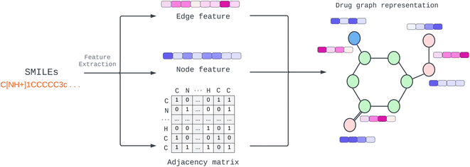
Provided by the benchmark datasets, our input drug compound is in SMILES format, and we utilized TorchDrug²³ and RDKit library²⁴ to extract node feature, edge features, and adjacency lists from drug SMILES to generate a graph as illustrated in Fig. 1. We represented node and edge features as shown in Table 1 with one-hot vectors (see ESI Table S1† for detailed features). Edge features make our data more elaborate and informative. In contrast, earlier work only used edges to connect nodes or weighted edges to express an edge's importance. Other work, for example, RGCN,²⁵ proposed using independent weight computation for different edge types.

Fig. 1 Construction of drug molecular graph with multidimensional edge feature.

Table 1 Node and edge one-hot features for drug representation

Feature	Size
Node features	(66)
Atomic symbol	18
Atomic chiral tag	4
degree of atom	8
Number of formal charge	11
Number of explicit and implicit Hs	7
Number of radical electron	8
Atom hybridization	8
Is aromatic	1
Is in ring	1
Edge features	(18)
Bond type	4
Bond direction	7
Bond stereo configuration	6
Bond is conjugated	1

---

We employed a multidimensional edge feature in this study to pass additional information to each convolution layer. The edge characteristics comprise bond type, bond stereo, and stereo atom, and the drug compound graph is a symmetric network representing a bidirectional graph for our configuration. To capture comprehensive information, including both the neighborhood and the individual node itself, we incorporated self-loops for all nodes in the graph. This self-loop ensures that the model learns the state embedding, which contains the surrounding nodes' context and the node's features.

2.3 Protein representation

One of the most difficult protein-related issues is how we can extract helpful protein features based on only its sequence. In contrast to drugs, whose structure information is given in SMILES format, proteins are considerably more complex. Although we can independently extract protein characteristics based on each amino acid property, such as residue-symbol, aliphatic, and polarity, the function is altered when amino acids link together and form a complex structure. Therefore, in this study, we adopted a pre-trained model known as “Evolutionary Scale Modeling” or ESM,²⁶ a transformer protein language model, to extract valuable and dependable protein features from its sequence (details in Pre-trained protein language section).

Many proteins have unknown structures. To extract structural information, we require a very complex model, such as AlphaFold,²⁷ which is resource-intensive to yield a precise result. In addition, prior work learned patterns from protein sequences using CNN or NLP, whereas other structural models used the predicted protein structure of other trained models. This paper proposes a novel way to solve the fixed-length problem of CNN and NLP using a GNN. First, we establish a pseudo-structure in which each amino acid represents a node and create an edge from its adjacency node in the sequence. This pseudo-structure allows us to utilize graph message-passing operations in a sequence string. We illustrate the process of protein graph construction in Fig. 2.

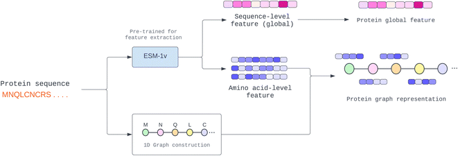Fig. 2 Construction of protein 1D graph representation where amino acid-level feature (node feature) and sequence-level feature (global feature) are extracted from the pre-trained model.

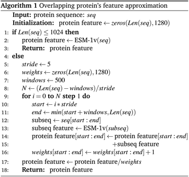
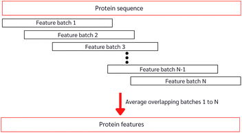
With the constrained sequence length to be fewer than 1024 amino acids of the ESM, while about 20–25% of our protein sequences comprise more than 1024 amino acids (ESI Fig. S1†), we must introduce a way to approximate long-sequence protein feature. Our approach divided a protein sequence into several pieces to make sub-sequences, where one sub-sequence with a fixed length of 500 (windows) and a step of 5 (stride), having 495 amino acids overlapping with the consecutive sub-sequence for a better approximation, and the final sequence feature being the average of all sub-sequences as described in Algorithm 1 and depicted in Fig. 3.

Fig. 3 Long-sequence protein feature approximation from the pre-trained model.

2.4 Pre-trained protein language

To achieve a more accurate representation of a protein sequence than its amino acid features, we employed a model that has been pre-trained with a vast amount of protein data and can predict a node feature from a protein sequence.

In our study, we conducted experiments using two pre-trained models, namely ProtTrans²⁸ and Evolutionary Scale Modeling (ESM).²⁶ The findings of these experiments are presented in the Module analysis section. Both pre-trained models employ a self-supervised transformer-based model with masking, in which each input token is corrupted by randomly substituting an amino acid with a unique token. Then, they were trained to predict the missing token from the corrupted sequence to learn a pre-training task.

ProtTrans²⁸ is a language model taken from the NLP technique. It has many variants, and the one we experimented on was the T5-XL model, an encoder-decoder model trained on the BFD dataset^29,30 and fine-tuned on the UniRef50 dataset,³¹ which contains 2122 and 45 million protein sequences, respectively. The T5-XL model extracts protein features by employing a transformer model and predicting token-level and protein-level classification tasks. We extracted the embedding features with 1024 dimensions per residue from the last hidden layer before predicting both tasks of the transformer model.

ESM²⁶ is also a transformer-based language model developed by Facebook research, trained on only the UniRef90 dataset³² comprising 98 million diverse protein sequences with 1280 dimensions of embedded features per residue. However, ESM has a restriction on sequence length, as it was trained with a fixed context size of 1024 tokens for positional embedding. Therefore, for protein sequences that are longer than 1024 amino acids, they used the random crop to reduce the protein sequence length to 1024 tokens for every training epoch to get sample sequences.

2.5 Model architecture

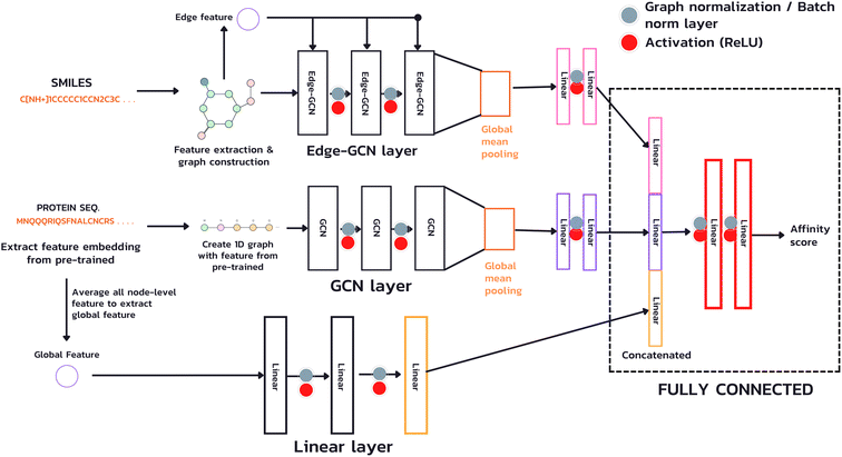
The model used in our study takes both inputs, a protein sequence and a drug compound in SMILES format, and transforms them into graph structures (Fig. 4). The drug branch (Edge-GCN layer) creates a graph using an actual contact, e.g., the graph's edges representing bonds between two atoms. On the other hand, the protein branch (GCN layer) creates a 1D graph from its sequence by sequentially connecting each amino acid to its adjacent neighbors instead of an actual contact, which is a complex piece of information. Instead of employing a fixed-length technique, such as padding or truncating, which is necessary for CNN and NLP, we used the whole sequence for feature extraction and model calculation with the GNN technique, which accepts an arbitrary-length input. Furthermore, due to the potentially extensive length of protein sequences, which requires a vast number of GCN layers to acquire information from the entire sequence (a single GCN layer can only gather information from neighboring nodes within one hop), we introduced an additional branch (Linear layer) for extracting a global feature, a sequence level feature. This feature is achieved by averaging the node-level features from the sub-sequences of the entire sequence and passing them through a linear layer to learn a comprehensive representation.

Fig. 4 The architecture of proposed model.

In this study, our focus is on predicting affinity scores, which are continuous values. To accomplish this, we employed GCN as a layer for feature extraction to produce the node-level representation of both drug and protein, using sequence-level features to create the whole protein sequence representation and a fully connected layer to gather information and produce the predicted affinity scores.

2.5.1 Graph neural network. Convolutional Neural Network (CNN) is widely used in many tasks involving data in Euclidean space, such as 1D (sequence) or 2D (grid) data, but in a task with non-euclidean data like a graph, we need a new method to handle this. Due to their capacity to handle graph structure data, GNN have recently garnered a great deal of attention, and several graph data types, such as social networks and drug-protein graphs, have become popular. This paper focuses on one of the variations of GNN that apply convolution over a graph, the Graph Convolutional Network (GCN),¹⁹ initially developed to address semi-supervised tasks like node classification. In this work, we will use GCN for graph-level feature extraction. The propagation rule of GCN consists of message passing, aggregate, and feature update, formulated as eqn (1),¹⁹ and illustrated in Fig. 5A.where à is an adjacency matrix of a graph with a self-loop connection. D̃ is the diagonal node degree matrix of à in measuring the degree of each node to maintain the scale of the output feature vector, while H^(l) is a previous hidden layer output. W^(l) represents learnable parameters, and σ is an activation function such as the Rectified Linear Unit (ReLU).

Fig. 5 (A) Example of the propagation rule on node v₁ in a GCN layer, where h_i is a hidden state of node i, and W is the learnable weight that transforms the aggregated output into a new hidden state . (B) Example of the propagation rule on node v₁ in our Edge-GCN layer, where h_i is a hidden state of node i, e_i is an edge feature of node i, and W is the learnable weight that transforms the aggregated output into a new hidden state .

2.5.2 Graph convolutional network with edge feature. To better represent a drug graph with a multi-dimensional edge feature from the preprocessing stage, we improved a graph message passing by including an edge feature in every convolution step as part of the GCN propagation rule in eqn (2) called Edge-GCN illustrated in Fig. 5B.

In which H^(l) in eqn (1) is replaced with H^(l) + EW^(l)_e, where E is a multi-dimensional edge feature and W^(l)_e is a learnable parameter that transforms the dimension of an edge feature into the dimension of a node feature. Note that the edge in the drug graph is undirected, which means that the connected nodes utilize the same edge feature for message propagation.

In our architecture, we transformed drug SMILES and protein sequences into a graph before giving them to two GCNs, each consisting of a three-layer convolutional network for extracting a representation from a graph. A global pooling layer is placed after the two GCNs to ensure that a graph-level representation with the same dimension is obtained. Each operation may be regarded as a hyperparameter when calculating a global pooling layer as a sum, mean, or max. In this work, we used the global mean pooling layer, eqn (3), where x is a feature matrix for each node in the GCN output. N is the number of nodes in the sequence, and r is the pooling output representation with a size of (1, F), where F is the number of output channels for the last layer.

2.5.3 Protein global feature. Since a protein is a highly complicated substance, it is challenging to discern its general function from node-level data. Since a pre-trained model learned from an extensive model and dataset, we considered extracting the global feature by averaging a node feature from a pre-trained to obtain a per-sequence feature with 1280 dimensions for each sequence, which then passed through three fully connected layers before being concatenated to the structural representation of drug and protein.

We added batch normalization (BatchNorm)³³ after every output layer in fully connected layers and graph normalization (GraphNorm)³⁴ for GCN layers, each activated by the Rectified Linear Unit (ReLU) function. We then concatenated the representation of the drug's latent feature, protein's latent feature, and protein's global feature to two fully connected layers to predict an affinity score.

2.5.4 Loss function and hyperparameter tuning. Our task is to minimize the affinity score difference between our model prediction and ground truth label during training. Since our task is a regression task, we use mean square error (MSE) as a loss function, which is calculated as the summed square of the difference between the predicted value (P) and ground truth label (Y), as shown in eqn (4).

We optimized our model via AdamW³⁵ optimization algorithm, which improves regularization in Adam by decoupling the weight decay from the gradient update. We set a weight decay parameter as 0.01 for both datasets to prevent overfitting. In addition, we used the learning rate decay, starting from 0.001 and decaying by scaling down to 80% for every 100 epochs to improve the learning of complex patterns in the late iteration process.

We tuned most of the hyperparameters manually and selected some others from the prior work, as shown in Table 2 as we employed cross-validation techniques, and the training process took a significant amount of time to complete.

Table 2 Hyperparameters setting for our model

Hyperparameter	Setting
Epoch	1000
Optimizer	AdamW
Batchsize	128
Learning rate	0.001
Weight decay	0.01
Dropout rate	0 (see batch normalization)
Latent size after GCN	128

---

3 Results and discussion

We used Nvidia DGX A100 for training and testing and built our model with PyTorch and PyTorch Geometric (PyG),³⁶ conducted model comparisons and selections based on five-fold cross-validation, and chose a candidate model to evaluate the performance over the independence test set. First, we selected the candidate model with the best result averaged from the validation set result of each fold and then evaluated the candidate model by using each fold's weight for predicting the independent test set (unseen data). Then, we calculated the final result by averaging the test results obtained from each fold. Note that we used the training part of each fold, excluding the validation part, to train the model for final evaluation (see ESI Fig. S2†).

3.1 Evaluation metrics

We implemented the same metrics used by the baseline and state-of-the-art methods to make our work comparable. Since we are working on a regression problem, we used MSE and Concordance Index (CI) as the primary metrics of the DTA task. MSE is a prevalent metric used in regression tasks. It measures the difference between the predicted and actual values. A smaller MSE means the predicted value from our model is closer to the true value. Unlike MSE, the CI score is interested in the order of predictions, not the prediction value itself, and calculated by eqn (5), where b_i is the prediction value for the larger affinity d_i, b_j is the prediction value for the smaller affinity d_j, Z is a normalization constant, and h(x) is the step function as shown in eqn (6).

Another metric used by some work is the Pearson correlation coefficient, eqn (7), which measures the strength of the linear relationship between two variables, predicted and ground truth in our case, where cov is the covariance between the predicted value p and the actual value y, and σ(p), σ(y) indicates the standard deviation of the predicted p and actual y respectively.

3.2 Benchmarking with the state-of-the-art models

We compared our method with the previous works. To make a fair comparison, we tested the performance with the unseen data on the independent test set and reported the same evaluation metrics, including MSE, CI, and Pearson correlation coefficient with standard deviation. Note that due to different evaluation settings, we reproduced the final result of some previous work in this benchmarking section and also provided the original results reported in their papers along with the modified evaluation of our model based on their setting in ESI Table S2.†

Tables 3 and 4 show the benchmarking results of our model compared with other methods, differently representing drug compounds and proteins, including CNN-based, graph-based, and transformer. Our technique combining Edge-GCN and 1D-GCN achieved considerable improvements in MSE and CI on the Davis dataset, reaching 0.216 for MSE, 0.897 for CI, and 0.855 for Pearson correlation on the independence test set. The KIBA dataset showed that our model outperformed other methods by having the lowest MSE and highest Pearson correlation. It also had the highest CI score among other graph-based methods (same rank as MGraphDTA), while SMT-DTA, a transformer-based model, had the highest CI score at 0.894. Our model is highly effective compared to the graph-based methods, e.g., GEFA, which previously got the lowest MSE of 0.228 on Davis. Notably, our model does not use protein structure compared to existing graph-based methods that extract protein graphs from contact map prediction, and our model still gets a better result. Therefore, it may imply that the pre-trained model, i.e., ESM, learned how proteins are formed or learned some structural information.

Table 3 Model performance on independence test set based on the Davis dataset

Model	Compound	Protein	MSE (std)	CI (std)	Pearson (std)
a These results were taken from our reproduction.
DeepDTA^11	CNN	CNN	0.261	0.878(0.004)	—
MT-DTI^12	Transformer	CNN	0.245	0.887(0.003)	—
GraphDTA^13^,^a	GIN	CNN	0.251(0.003)	0.882(0.003)	—
DGraphDTA^14^,^a	GCN	GCN(contact)	0.238(0.005)	0.888(0.004)	0.840(0.003)
GEFA^15	GCN	GCN(contact)	0.228	0.893	0.846
WGNN^16^,^a	GCN	WGCN(contact)	0.244(0.004)	0.888(0.002)	0.837(0.002)
MGraphDTA^17^,^a	MGNN	MCNN	0.233(0.005)	0.885(0.004)	0.843(0.004)
SMT-DTA^18	Transformer	Transformer	0.219	0.890	—
Our	Edge-GCN	1D-GCN	0.216(0.004)	0.897(0.001)	0.855(0.002)

---

Table 4 Model performance on independence test set based on the KIBA dataset

Model	Compound	Protein	MSE (std)	CI (std)	Pearson (std)
a These results were taken from our reproduction.
DeepDTA^11	CNN	CNN	0.194	0.863(0.002)	—
MT-DTI^12	Transformer	CNN	0.152	0.882(0.001)	—
GraphDTA^13^,^a	GAT&GCN	CNN	0.186(0.009)	0.871(0.001)	—
DGraphDTA^14^,^a	GCN	GCN(contact)	0.148(0.002)	0.889(0.002)	0.885(0.002)
MGraphDTA^17^,^a	MGNN	MCNN	0.150(0.004)	0.890(0.002)	0.883(0.003)
SMT-DTA^18	Transformer	Transformer	0.154	0.894	—
Our	Edge-GCN	1D-GCN	0.139(0.001)	0.890(0.001)	0.892(0.001)

---

3.3 Module analysis

3.3.1 Batch normalization. The implementation of batch normalization was an additional effective strategy we utilized to improve the regularization of our model. Deep learning commonly uses batch normalization to normalize the input data within each mini-batch during training. By normalizing the activations, batch normalization reduces the internal covariate shift, which is the phenomenon of a shift in the distribution of layer inputs as model parameters change. This stabilization effect helps the model converge more quickly. In addition, estimating expectations and variance from many small data subsets also provides a model's regularization effect.

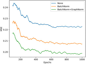
We illustrate the impact of batch normalization in Fig. 6. During the early epochs before the red dashed line, the model incorporating batch normalization exhibits faster convergence than the model without. However, in the later epochs, the model's mean squared error (MSE) without batch normalization decreases, indicating a better fit to the training set. Nevertheless, the results on the validation set depicted in Fig. 7 reveal that the model without batch normalization performs worse than the other models, suggesting the presence of an overfitting issue and showing how the batch normalization helps generalize the model. In summary, we achieved additional regularization without a dropout layer by incorporating batch normalization into our model, expedited the training process, and improved overall performance (see ESI Fig. S3† for the performance of the dropout layer).

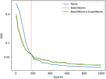Fig. 6 Training performance of the model with different batch normalization setting, the model without batch normalization (blue) get the best performance in training set (lower is better).

Fig. 7 Validation performance of the model with different batch normalization settings, the model with both BatchNorm and GraphNorm (green) gets the best performance in validation set (lower is better).

3.3.2 Pre-trained models. This study aims to apply graph neural network to a protein based on the protein's sequence, assuming that we cannot obtain the actual or predicted protein structure. Therefore, it would be best to utilize a pre-trained model because it has learned a massive dataset and might implicitly store some information about the protein structure. Consequently, we chose two pre-trained models to create a protein input feature for our model and evaluated their prediction performance on the Davis dataset, as shown in Table 5.

Table 5 Performance of model component on average five-fold Davis's cross validation set

Model	MSE (std)	CI (std)
Baseline (DgraphDTA)	0.212(0.006)	0.885(0.004)
Pre-trained choice
ProtT5	0.206(0.008)	0.895(0.005)
ESM-1v	0.202(0.007)	0.897(0.005)
Edge feature
ESM-1v w/o edge feature	0.202(0.007)	0.897(0.005)
ESM-1v w/edge feature	0.198(0.006)	0.899(0.002)
Protein global feature
ESM-1v w/edge feature	0.198(0.006)	0.899(0.002)
iEdgeDTA(ESM + edge + global)	0.195(0.005)	0.901(0.002)

---

The findings indicated that both pre-trained models performed better than the baseline model (DGraphDTA), which relied on manually crafted features for protein representation. However, ESM-1v provided superior performance to PortT5, where the MSE value was 0.201, and the CI value was 0.898. As a result, we selected ESM-1v as our pre-trained model for final evaluation.

3.3.3 Edge and global features. Since we could extract an edge feature of the drug compound, we also passed it to our modified GNN model to include the edge feature for every message-passing process. However, extracting an edge feature for protein is still challenging. Hence, we instead pulled out an independent global feature by averaging its pre-trained node-level feature and learning to draw out a latent property via three dense layers. The performance of introducing the compound's edge and protein's global features into the model is shown in Table 5.

The results indicated that edge features on only the drug branch could improve the performance to achieve 0.198 for the MSE value and 0.899 for the CI value. Then, we assessed the performance of the protein's global feature, and the findings indicated that this feature also helped improve the prediction result, with MSE lowering to 0.195 and CI score increasing to 0.901 for the optimal iteration.

Besides, we compared our edge feature integration method to existing methods such as RGCN, which improves prediction by employing independent weights for each relation type rather than sharing weights across all nodes and edges. In this task, the bond type is passed as a relation type consisting of a single bond, double bond, triple bond, aromatic, and self-loop, resulting in five distinct weights. As shown in Table 6, utilizing RGCN does not increase model performance on a five-fold cross-validation set. This result may be related to our approach leveraging multidimensional edge features, whereas RGCN can only accept a single feature as the relation type.

Table 6 Comparison of the edge integration approach with a five-fold Davis's cross validation set

Model	Edge feature	MSE (std)
RGCN	Relation	0.201(0.006)
Our (GCN)	None	0.201(0.006)
Our (Edge-GCN)	Muti-dimension	0.198(0.006)

---

Furthermore, we incorporated our Edge-GCN approach into our baseline model, DGraphDTA, to assess the efficacy of integrating an edge feature into drug representations. In this experiment, we replaced the original GCN layers with our Edge-GCN layers in the drug branch, using the same edge feature introduced in this paper. The results are shown in Table 7, revealing that introducing an edge feature to the graph neural network improves both MSE and CI scores.

Table 7 Performance of applying an edge feature to DGraphDTA model on five-fold Davis's cross validation set

Model	MSE (std)	CI (std)
DGraphDTA	0.212(0.007)	0.888(0.004)
w/Edge-GCN	0.207(0.006)	0.895(0.002)

---

To assess the impact of individual contributions of node-level and sequence-level features for protein feature extraction, we selected a CNN architecture as our baseline due to its prevalence in prior studies and its suitability for assessing the effectiveness of our 1D-GCN in addressing the fixed-length problem. We set the hyperparameters of the CNN following GraphDTA¹³ work. Specifically, we fixed the protein sequence length at 1000 amino acids, padded shorter sequences, and truncated longer sequences. In Table 8, we present the results obtained from the experiment, showing the performance of the individual node-level and sequence-level features as standalone versions. These results demonstrate the improvement achieved by each feature independently and highlight their respective contributions. Moreover, integrating both node-level and sequence-level features within the 1D-GCN model yielded significant enhancements, surpassing the performance of the baseline model. This outcome shows the benefits of combining these features, further improving prediction accuracy.

Table 8 Individual contribution of node-level and sequence level feature with a CNN baseline model on five-fold Davis's cross validation set

Model	Method	MSE (std)	CI (std)
CNN baseline	CNN	0.210(0.007)	0.891(0.003)
Node feature	1D-GCN	0.198(0.005)	0.899(0.002)
Global feature	Linear	0.202(0.005)	0.896(0.003)
iEdgeDTA	1D-GCN + Linear	0.195(0.005)	0.901(0.002)

---

3.3.4 Contact map performance. Lastly, we conducted an additional analysis to investigate the influence of protein structure on our model. Specifically, we replaced a 1D sequence graph with a contact map obtained from various contact map model predictions. For this experiment, we selected three works: pconsc4,^14,37 utilized by our baseline model DGraphDTA, RaptorX³⁸ employed by GEFA, and the ESM²⁶ contact map prediction model. These models provide a probability indicating the likelihood of an amino acid pair being in contact, where contact determination is based on a threshold set as 0.5. To conduct this analysis, we maintained consistent model architecture and froze all hyperparameters while modifying the construction of the protein graph. Additionally, we employed our 1D sequence graph in the DGraphDTA model to assess the impact of 1D-GCN in a different model setting. The results of this analysis are presented in Table 9.

Table 9 Performance of 1D-GCN compared with predicted contact map from various contact map prediction models on average five-fold Davis's cross validation set

Contact map model	MSE (std)	CI (std)
DGraphDTA
pconsc4	0.212(0.006)	0.885(0.004)
1D-GCN	0.211(0.007)	0.893(0.001)
iEdgeDTA
pconsc4	0.197(0.005)	0.901(0.003)
RaptorX	0.196(0.006)	0.899(0.004)
ESM	0.198(0.004)	0.900(0.004)
1D-GCN	0.195(0.005)	0.901(0.002)

---

Our findings revealed that the performance of the 1D-GCN setting is on par with that of a model utilizing a contact map. Furthermore, the 1D-GCN approach exhibited slightly superior performance in our work and the DGraphDTA experiment compared to the contact maps derived from other prediction models. These results indicated that the structural information obtained from contact map predictions might contain noise that could potentially degrade model performance, suggesting that achieving enhanced performance requires either a genuine contact map or highly accurate predictions. Nonetheless, our comparative evaluation highlights that the 1D-GCN approach delivers similar performance without using contact maps. Moreover, given that actual protein contact maps are a limited resource, generating experimentally determined contact maps for proteins can be difficult and time-consuming, requiring specific equipment, specialized knowledge, and substantial resources, making them less accessible and limited to specific research facilities. Many strategies employ machine learning algorithms or statistical methods to infer residue–residue contacts based on the available protein sequence. However, due to the complexity of the nature of proteins, accurately predicting contact maps remains a challenging problem that requires substantial computational resources. Our model holds promise for real-world applications, such as high-throughput virtual screening, using only protein sequences.

However, iEdgeDTA does have limitations. First, using a 1D representation poses a drawback, as the protein's folding determines the binding pocket, and the 1D model does not guarantee that the binding pocket will correspond to a series of adjacent amino acids in the sequence string. Therefore, visualizing or predicting the binding pocket solely from the 1D representation remains a challenging problem. Second, a limitation lies in the pre-trained model, which may generate noise during extracting long protein sequences, as estimated in Algorithm 1. Using a more accurate pre-trained model that can handle arbitrary sequence lengths will reduce the model's sensitivity to noise, which may improve its performance.

4 Conclusions

Accurate drug target affinity prediction is essential for identifying promising candidates in developing and optimizing the design of new drugs. It can also help reduce drug discovery costs and time via drug repositioning to assess if existing drugs can bind to a specific protein target. In this study, we introduced a graph-based deep learning model that enhanced the prediction performance by incorporating background knowledge, adding a multidimensional edge feature, and using a more complicated node feature of proteins from the pre-trained model. By comparing the performance of our model to other recent research employing a range of methodologies, we found that our method improves prediction accuracy. In addition, we evaluated the effectiveness of our model when we included protein structure based on a contact map, and the results indicated that protein structure is optional for our model to achieve good prediction accuracy. As our model only incorporates an edge feature in the drug branch, future work could improve the model's accuracy by enhancing the protein node and edge feature extraction.

Author contributions

N. N. primarily designed the study and supervised model development and testing. D. W. supervised the overall research project and reviewed and provided valuable feedback on the manuscript, contributing to its improvement. The original draft was written by N.N. and reviewed/edited by D. W.

Data availability

https://github.com/cucpbioinfo/iEdgeDTA

Conflicts of interest

There are no conflicts to declare.

Acknowledgements

This work was partially supported by the National Research Council of Thailand (NRCT) under contract number N34A640454 and the Program Management Unit for Competitiveness (PMU-C), Office of National Higher Education Science Research and Innovation Policy Council, Thailand, under contract number C10F640366. We want to thank Chulalongkorn University Technology Center (UTC) for facilitating the GPU infrastructure for our model development and testing.

Notes and references

1. Y. L. Ng, C. K. Salim and J. J. H. Chu, Pharmacol. Ther., 2021, 228, 107930.
2. W. D. Jang, S. Jeon, S. Kim and S. Y. Lee, Proc. Natl. Acad. Sci. U. S. A., 2021, 118, e2024302118.
3. A. Khataniar, U. Pathak, S. Rajkhowa and A. N. Jha, COVID, 2022, 2, 148–167.
4. M. Thafar, A. B. Raies, S. Albaradei, M. Essack and V. B. Bajic, Front. Chem., 2019, 7, 782.
5. T. N. Jarada, J. G. Rokne and R. Alhajj, J. Cheminf., 2020, 12, 46.
6. T. T. Ashburn and K. B. Thor, Nat. Rev. Drug Discovery, 2004, 3, 673–683.
7. A. Mullard, Nat. Rev. Drug Discovery, 2014, 13, 877.
8. M. C. Cobanoglu, C. Liu, F. Hu, Z. N. Oltvai and I. Bahar, J. Chem. Inf. Model., 2013, 53, 3399–3409.
9. D.-S. Cao, L.-X. Zhang, G.-S. Tan, Z. Xiang, W.-B. Zeng, Q.-S. Xu and A. F. Chen, Mol. Inf., 2014, 33, 669–681.
10. H. Öztürk, E. Ozkirimli and A. Özgür, BMC Bioinf., 2016, 17, 128.
11. H. Öztürk, A. Özgür and E. Ozkirimli, Bioinformatics, 2018, 34, i821–i829.
12. B. Shin, S. Park, K. Kang and J. C. Ho, Proceedings of the 4th Machine Learning for Healthcare Conference, 2019, pp. 230–248.
13. T. Nguyen, H. Le, T. P. Quinn, T. Nguyen, T. D. Le and S. Venkatesh, Bioinformatics, 2020, 37, 1140–1147.
14. M. Jiang, Z. Li, S. Zhang, S. Wang, X. Wang, Q. Yuan and Z. Wei, RSC Adv., 2020, 10, 20701–20712.
15. T. M. Nguyen, T. Nguyen, T. M. Le and T. Tran, IEEE/ACM Trans. Comput. Biol. Bioinf., 2022, 19, 718–728.
16. M. Jiang, S. Wang, S. Zhang, W. Zhou, Y. Zhang and Z. Li, BMC Genomics, 2022, 23, 449.
17. Z. Yang, W. Zhong, L. Zhao and C. Yu-Chian Chen, Chem. Sci., 2022, 13, 816–833.
18. Q. Pei, L. Wu, J. Zhu, Y. Xia, S. Xie, T. Qin, H. Liu and T.-Y. Liu, SMT-DTA: Improving Drug-Target Affinity Prediction with Semi-supervised Multi-task Training, arXiv, 2022, preprint, arXiv:2206.09818,  DOI:10.48550/arXiv.2206.09818.
19. T. N. Kipf and M. Welling, Proceedings of the 5th International Conference on Learning Representations, 2017.
20. M. I. Davis, J. P. Hunt, S. Herrgard, P. Ciceri, L. M. Wodicka, G. Pallares, M. Hocker, D. K. Treiber and P. P. Zarrinkar, Nat. Biotechnol., 2011, 29, 1046–1051.
21. J. Tang, A. Szwajda, S. Shakyawar, T. Xu, P. Hintsanen, K. Wennerberg and T. Aittokallio, J. Chem. Inf. Model., 2014, 54, 735–743.
22. T. He, M. Heidemeyer, F. Ban, A. Cherkasov and M. Ester, J. Cheminf., 2017, 9, 24.
23. Z. Zhu, C. Shi, Z. Zhang, S. Liu, M. Xu, X. Yuan, Y. Zhang, J. Chen, H. Cai, J. Lu, C. Ma, R. Liu, L.-P. Xhonneux, M. Qu and J. Tang, 2022, preprint, arXiv:2202.08320,  DOI:10.48550/arXiv.2202.08320.
24. G. Landrum, P. Tosco, B. Kelley, D. Ric, R. Vianello, N. Schneider, E. Kawashima, D. N, A. Dalke, G. Jones, B. Cole, M. Swain, S. Turk, A. Savelyev, A. Vaucher, M. Wójcikowski, I. Take, D. Probst, V. F. Scalfani, K. Ujihara, G. Godin, A. Pahl and F. Berenger, JLVarjo, jasondbiggs, strets123 and JP, rdkit/rdkit: 2022_09_5 (Q32022) Release, 2023,  DOI:10.5281/zenodo.7671152.
25. M. Schlichtkrull, T. N. Kipf, P. Bloem, R. van den Berg, I. Titov and M. Welling, The Semantic Web, ESWC 2018, Lecture Notes in Computer Science, ed. A. Gangemi et al., Springer, Cham, 2018, vol. 10843,  DOI:10.1007/978-3-319-93417-4_38.
26. J. Meier, R. Rao, R. Verkuil, J. Liu, T. Sercu and A. Rives, bioRxiv, 2021, preprint,  DOI:10.1101/2021.07.09.450648.
27. J. Jumper, R. Evans, A. Pritzel, T. Green, M. Figurnov, O. Ronneberger, K. Tunyasuvunakool, R. Bates, A. Žídek, A. Potapenko, A. Bridgland, C. Meyer, S. A. A. Kohl, A. J. Ballard, A. Cowie, B. Romera-Paredes, S. Nikolov, R. Jain, J. Adler, T. Back, S. Petersen, D. Reiman, E. Clancy, M. Zielinski, M. Steinegger, M. Pacholska, T. Berghammer, S. Bodenstein, D. Silver, O. Vinyals, A. W. Senior, K. Kavukcuoglu, P. Kohli and D. Hassabis, Nature, 2021, 596, 583–589.
28. A. Elnaggar, M. Heinzinger, C. Dallago, G. Rehawi, W. Yu, L. Jones, T. Gibbs, T. Feher, C. Angerer, M. Steinegger, D. Bhowmik and B. Rost, IEEE Trans. Pattern Anal. Mach. Intell., 2021, 1.
29. M. Steinegger and J. Söding, Nat. Commun., 2018, 9, 2542.
30. M. Steinegger, M. Mirdita and J. Söding, Nat. Methods, 2019, 16, 603–606.
31. B. E. Suzek, Y. Wang, H. Huang, P. B. McGarvey and C. H. Wu, The UniProt Consortium, Bioinformatics, 2014, 31, 926–932.
32. B. E. Suzek, H. Huang, P. McGarvey, R. Mazumder and C. H. Wu, Bioinformatics, 2007, 23, 1282–1288.
33. S. Ioffe and C. Szegedy, Proceedings of the 32nd International Conference on International Conference on Machine Learning, 2015, vol. 37, pp. 448–456.
34. T. Cai, S. Luo, K. Xu, D. He, T. yan Liu and L. Wang, GraphNorm: A Principled Approach to Accelerating Graph Neural Network Training, 2020.
35. I. Loshchilov and F. Hutter, Decoupled Weight Decay Regularization, arXiv, 2017, preprint, arXiv:1711.05101,  DOI:10.48550/arXiv.1711.05101.
36. M. Fey and J. E. Lenssen, ICLR Workshop on Representation Learning on Graphs and Manifolds, 2019.
37. M. Michel, D. Menéndez Hurtado and A. Elofsson, Bioinformatics, 2018, 35, 2677–2679.
38. S. Wang, S. Sun, Z. Li, R. Zhang and J. Xu, PLoS Comput. Biol., 2017, 13, 1–34.

---

Footnote

† Electronic supplementary information (ESI) available: Detailed drug feature, performance of iEdgeDTA evaluated in the same setting as reproduced previous work, dataset distribution, graphical explanation of cross-validation and testing, performance of dropout layers. See DOI: https://doi.org/10.1039/d3ra03796g

---