
 Open Access Article
 This Open Access Article is licensed under a Creative Commons Attribution-Non Commercial 3.0 Unported Licence
Magnetocaloric effect and critical behavior of the La0.75Ca0.1Na0.15MnO3 compound
Souhir Bouzidi *a,
Mohamed Hsinib,
Sonia Soltanic,
Manel Essidd,
M. A. Albedahe,
Hafedh Belmabrouke and
J. Dhahria
*a,
Mohamed Hsinib,
Sonia Soltanic,
Manel Essidd,
M. A. Albedahe,
Hafedh Belmabrouke and
J. Dhahria
aLaboratoire de La Matière Condensée et des Nanosciences, Département de Physique, Faculté des Sciences de Monastir, Avenue de L’Environnement Monastir, 5019 Monastir, Tunisia. E-mail: Souhirbouzidi@outlook.com
bLaboratory of Physical Chemistry of Materials, Faculty of Science of Monastir, Department of Physics, University of Monastir, 5019 Monastir, Tunisia
cDepartment of Physics, College of Science and Arts, Qassim University, Dariyah 58251, Saudi Arabia
dChemistry Department, College of Science, King Khalid University (KKU), P.O. Box 9004, Abha, Saudi Arabia
eDepartment of Physics, College of Science, Majmaah University, Al Majma'ah, 11952, Saudi Arabia
First published on 1st June 2023
Abstract
In this paper, we have studied the critical behavior and the magnetocaloric effect (MCE) simulation for the La0.75Ca0.1Na0.15MnO3 (LCNMO) compound at the second order ferromagnetic–paramagnetic phase transition. The optimized critical exponents, based on the Kouvel–Fisher method, were found to be: β = 0.48 and γ = 1. These obtained values supposed that the Mean Field Model (MFM) is the proper model to analyze adequately the MCE in the LCNMO sample. The isothermal magnetization M(H, T) and the magnetic entropy change −ΔSM(H, T) curves were successfully simulated using three models, namely the Arrott–Noakes equation (ANE) of state, Landau theory, and MFM. The framework of the MFM allows us to estimate magnetic entropy variation in a wide temperature range within the thermodynamics of the model and without using the usual numerical integration of Maxwell relation.
1 Introduction
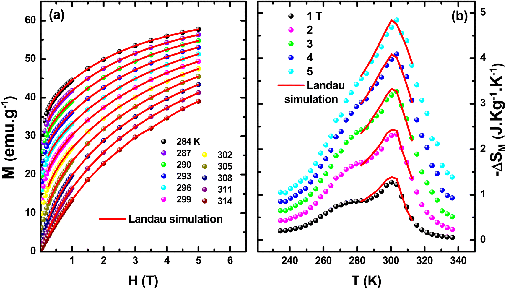
The ferromagnetic (FM)–paramagnetic (PM) second-order phase transition is one of the most advanced issues in terms of functionality and fundamental physics of magnetic materials. As an advanced research interest, it is important to analyze the magnetocaloric effect when evaluating the effectiveness of magnetic refrigerators, which should be more economical and environmentally friendly.1–3 Therefore, the second-order ferromagnetic–paramagnetic phase transition may be discussed based on the concept of critical behavior that links several thermodynamic properties of the magnetic system.Around the FM–PM, various phase-transition measurable quantities can be determined using a series of critical exponents defining the behavior of these magnetic materials.4–7 The design and development of magnetic refrigeration devices require a solid thermodynamic description of the magnetic system, as well as its characteristics during each phase of the refrigeration cycle. Recently the magnetic properties and the magnetocaloric effect (MCE) for La0.75Ca0.1Na0.15MnO3 (LCNMO) manganite undergoing a second order (SO) FM–PM phase transition, were reported in our previous work.8 Near room temperature, the LCNMO sample exhibits a large magnetic entropy change with maxima of 4.83 J kg−1 K−1 and a high relative cooling power of 230 J kg−1 under 5 T magnetic field. These results suggest that the LCNMO sample could be promising candidates for magnetic refrigeration.
Several numerical methods9–12 can be exploited to solve the non-algebraic equation relating the magnetization M(H, T) to the applied magnetic field H and the temperature T in the ferromagnetic material. The utility of theoretically efficient methods can be exploited to simplify data analysis. However, the magnetic entropy change, −ΔSM(H, T) is governed by H, T, the magnetic field variation (ΔH), the temperature variation (ΔT) and M(H, T) data. As a result, choosing H, T, ΔH, and ΔT is important during evaluating the MCE of the magnetic material.
In this work, the critical behavior of LCNMO has been studied. Firstly, the critical exponents β and γ were calculated by an iterative method extended to the modified Arrot plot (MAP). The inverse of the magnetic susceptibility χ0−1(T) and the spontaneous magnetization Ms(T) were determined. Then, isothermal M(H, T) and −ΔSM(T) curves were generated by resolving the Arrott–Noakes equation (ANE) of state. Secondly, the use of the Landau model of phase transitions13–15 enables the simulation of M(H, T) and −ΔSM(T) curves. However, these two approaches (ANE and Landau theory) are valid only in a very narrow temperature region near the Curie temperature, TC. Thirdly, by analyzing the mean field equation, the M(H, T) and −ΔSM(T) plots of our studied LCNMO magnetic system are generated. Contrarily to what has been mentioned about the ANE and the Landau model, the dependence of M and −ΔSM on T, H can be described by using the Mean Field Model (MFM) in a large temperature region.
2 Results and discussions
The LCNMO manganite8 was prepared by the flux method. The crystallographic study revealed that the LCNMO compound is characterized by the coexistence of a mixture of orthorhombic and rhombohedral structures with Pbnm and R![[3 with combining macron]](https://www.rsc.org/images/entities/char_0033_0304.gif) c space groups, respectively. The magnetization data, under 0.05 T magnetic field proved that LCNMO exhibited a SO FM–PM near the room temperature (TC = 301.5 K).
c space groups, respectively. The magnetization data, under 0.05 T magnetic field proved that LCNMO exhibited a SO FM–PM near the room temperature (TC = 301.5 K).
2.1 Arrott–Noakes equation (ANE)
Overall, the ANE near the second-order ferromagnetic–paramagnetic transition is expressed as:16
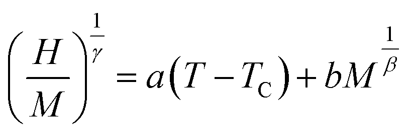 | (1) |
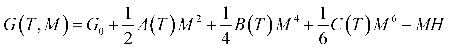
Using the thermodynamic relation 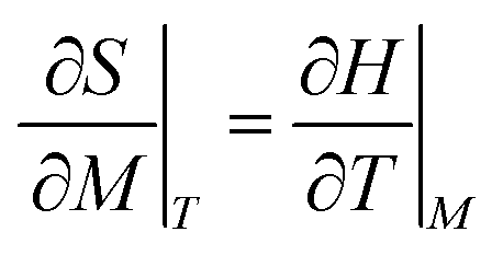 , the expression of −ΔSM(M) is given through eqn (1) by:17
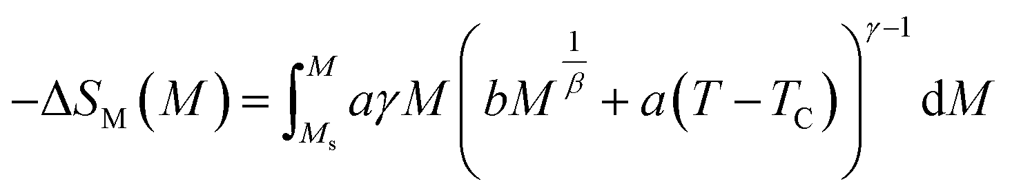 | (2) |
Basing on eqn (1), the initial magnetic susceptibility χ0 for T > TC and the spontaneous magnetization MS for T < TC are as follows:18
| MS = M0(−ε)β; T < TC, | (3) |
| χ0−1 = h0εγ; T > TC, | (4) |
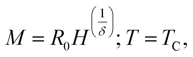 | (5) |
 ,
,  is the reduced temperature, M0, h0 and R0 present critical amplitudes. The choice of β and γ values is adequate if it results in a parallel set of linear lines for the plot
  vs.
vs.  with the passing of the critical isotherm (at T = TC) from the origin. For T < TC, the abscissa intercepts correspond to MS1/β however for T > TC, the ordinate intercepts refer to (χ0−1)1/γ. The involvement of arbitrary critical exponents in eqn (1) may conduct to unacceptable fits and erroneous values of the exponents. For this reason, an implemented program based on a rigorous iterative method19 is often used to determine the values of the couple (β, γ) after starting with the initial MFM critical values (β = 0.5, γ = 1). After multiple iterations, a set of nearly parallel straight lines
  vs.
vs.  have been generated. In Fig. 1, we report the curves using the values: β = 0.48 and γ = 1.
 | ||
Fig. 1 Modified Arrot plot,  vs. vs.  , for La0.75Ca0.1Na0.15MnO3 (LCMNO) compound. , for La0.75Ca0.1Na0.15MnO3 (LCMNO) compound. | ||
It is evident in Fig. 1 that isothermal lines  vs.
vs.  were set under high magnetic fields (greater than H = 1 T). This is because isotherms are averaged and magnetized in different directions at lower magnetic fields.20 But, under high magnetic fields, all isotherms undergo parallel straight lines. The values of the critical exponent of LCMNO are close to those predicted by the MFM (β = 0.5, γ = 1). Linear fits of the MAP yield the MS1/β and (χ0−1)1/γ described above. The estimated data of MS(T) and χ0−1(T) are plotted in Fig. 2(a). Fitting MS(T) using eqn (3) gives the values of: β = 0.48 and TC = 301.49 K. Similarly, fitting χ0−1(T) using eqn (4) gives: γ = 1 and TC = 301.5 K. Since the experimental data of the critical isotherm M(H) at TC = 301.5 K is not available, the critical exponent δ is supposed to be restricted between M(H) at 299 and 302 K. temperature. The fit of the isotherms M(H, T = 299 K) and M(H, T = 302 K) with eqn (5) gives the respective values of δ as 3.46 and 2.86. Furthermore, this δ exponent may be also calculated from Widom scaling relation:21
  With the optimized values, β = 0.48 and γ = 1, δ = 3.08. It is obvious that the δ value is restricted between the ones calculated from the fit of isotherms M(H, T = 299 K) and M(H, T = 302 K) with eqn (5). As a result, the reliability of the estimated critical exponents was confirmed.
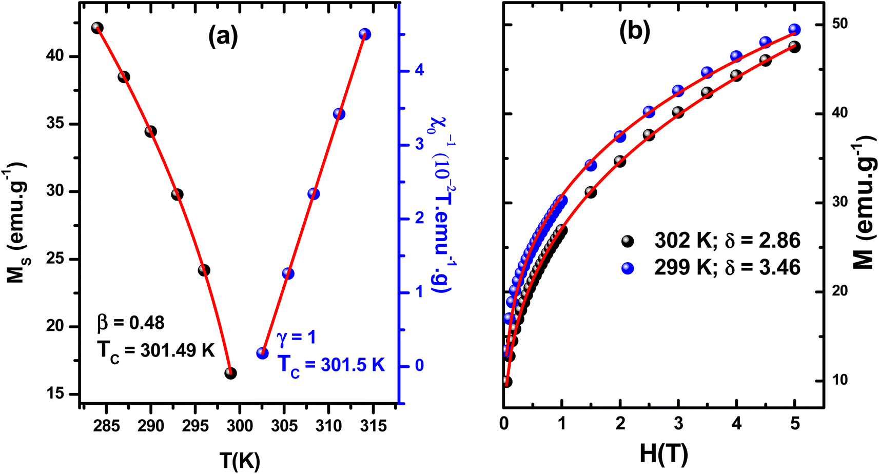 | ||
| Fig. 2 (a) Fitting of MS(T) and χ0−1(T), with eqn (3) and (4), respectively. (b) Fitting of M(H) at 299 and 302 K temperature with eqn (5), for LCMNO sample. | ||
For the LCMNO compound, the γ value matches the MFM suggesting that the FM–PM phase transition would belong to the MFM. Thus, the origin of this transition is explained by the long-range physical interaction. Moreover, for a system of dimension d and spin n, γ varies with extension of the interaction σ as:22 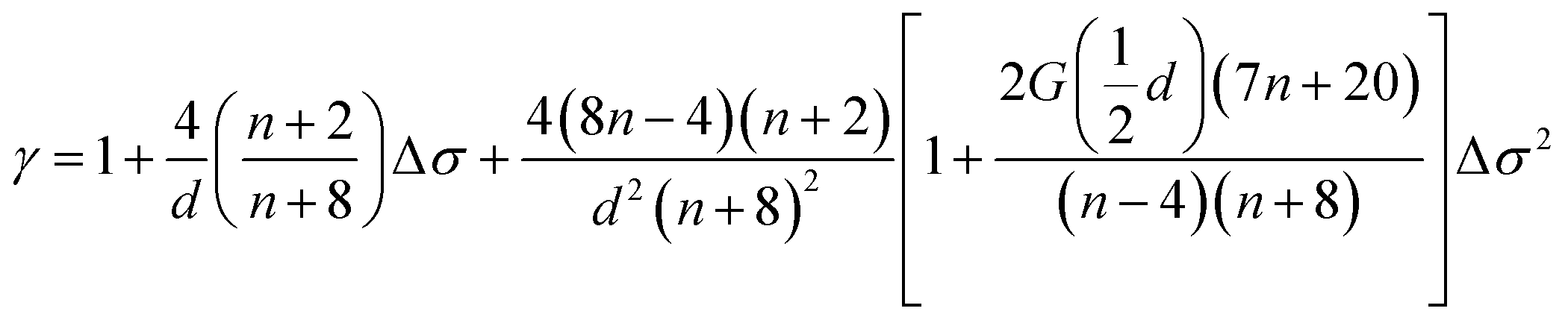 with
with 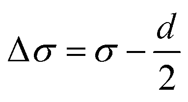 ;
; 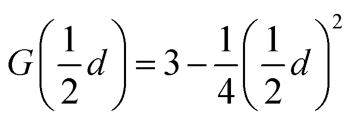 . The renormalization group study suggests that σ (or γ) indicates the exchange integral J(r) over a distance r as follows:23 J(r) ∼ r−(d+σ). For σ > 2 or σ < 2, we observe a 3D system of isotropic long- or short-range spins, respectively. The 3D Heisenberg model is correct if σ > 2, with J(r) decreasing at short distances faster than r−5. In our case (with γ = 1), σ ≈ 1.5; then J(r) decreases as r−4.5. Therefore, J(r) decreases more slowly than r−5 for LCMNO manganite as a function of long-range distance.
To simulate M(H, T) and −ΔSM(T, H) curves, around TC, we have first determined the constants a and b given in eqn (1) were firstly determined. The linear fits of  vs.
vs.  yield a(T − TC) at the interceptions of the axis
  . The quantity b represents the slope of
  vs.
vs. 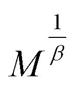 at TC. Both constants are calculated as: a = 0.0036 and b = 2.6 10−5 with units of M in emu g−1 and H in tesla.
Then the numerical resolution of eqn (1) generates M(H, T) plots (solid lines). A good agreement is observed with the experimental data mainly when H is greater than 1 T as presented in Fig. 3(a).
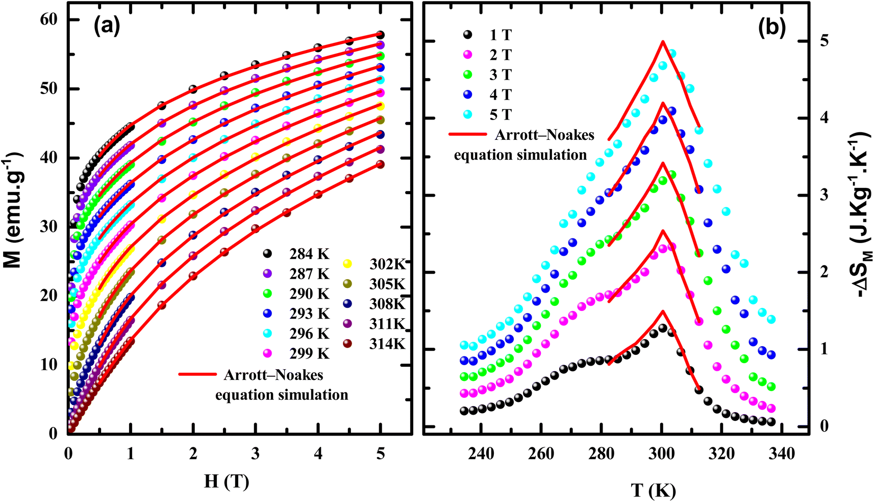 | ||
| Fig. 3 The experimental (red lines) and the simulated (symbols) curves of (a) M vs. H and (b) −ΔSM vs. T using the ANE. | ||
Using MS(T) and the generated values of M(H, T), a theoretical estimation of −ΔSM(T, H) can be obtained. These simulated −ΔSM curves (solid lines) correlated adequately with experimental −ΔSM curves which were evaluated using the well-known Maxwell relation 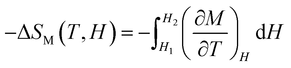 , as shown in Fig. 3(b). Although a reasonable correlation was obtained in the whole temperature, the simulated curves of −ΔSM(T) depart slightly from the experimental ones near TC. This shift is consistent with saturation effects not contemplated in the ANE.24
2.2 Landau theory
According to the Landau model, the Gibbs free energy can be written as follows:25
 | (6) |
 | (7) |
The variables A(T), B(T) and C(T) can be calculated from the quadratic fit of vs. M2.
The magnetic entropy is given as follows:
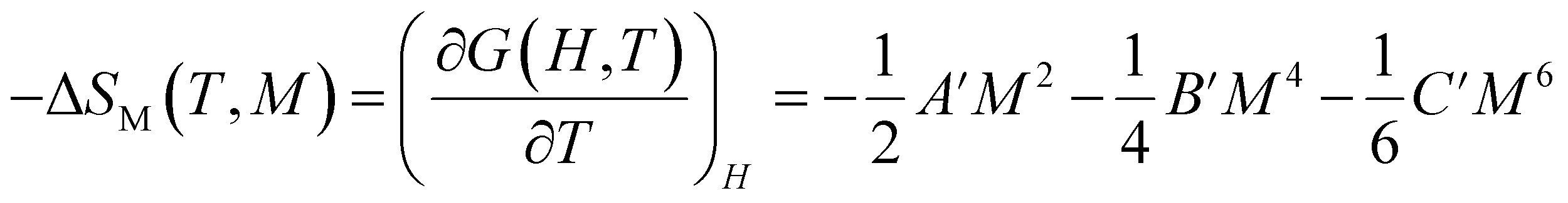 | (8) |
 ,
,  and
and  .
.
Using the renormalization group, Dong et al.26 pointed out that in the absence of the external magnetic field, −ΔSM(H = 0 T) should differ from zero since it is impacted by spontaneous magnetization. Therefore, eqn (8) should be adjusted as follows:
 | (9) |
The treatment of eqn (6) leads to the generation of M(H, T) plots which are represented by red lines and corroborate the experimental data when H is larger than 0.5 T as indicated in Fig. 4(a). Then, using generated M(H, T), obtained from eqn (6), and MS(T) in eqn (8), simulated −ΔSM curves can be determined. An acceptable concordance is achieved between the simulated −ΔSM curves (red lines) and the experimental −ΔSM curves (symbols) estimated by Maxwell's relations as given in Fig. 4(b).
 | ||
| Fig. 4 The experimental (symbols) and the simulated (red lines) curves of (a) M vs. H and (b) −ΔSM vs. T using the Landau theory. | ||
Some points can be discussed when comparing the ANE with its derivatives from one side and the Landau theory from the other side. These two approaches are valid only in a very narrow region: |ε| < 0.1.27 Since the critical behavior at the second FM–PM phase transition is studied at high magnetic field, under weak magnetic fields, the ANE has a limited ability to simulate the curves of magnetic compounds (in this study), we take the analysis starting from 1 T because of the inability to obtain parallel straight lines  vs.
vs. 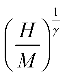 for the total applied magnetic field. Landau theory (which starts at 0.5 T) decreases this disability but is still unable to simulate M(H, T) curves under low magnetic fields.
2.3 Mean field model
The magnetization values can be expressed according to the MFM with respect to the saturation magnetization (M0) as28,29
 | (10) |
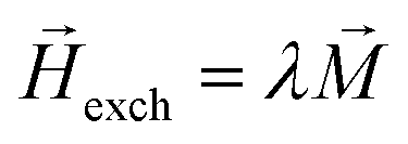 , λ is the exchange parameter.
Knowing that M is a function of  ; in other words,
 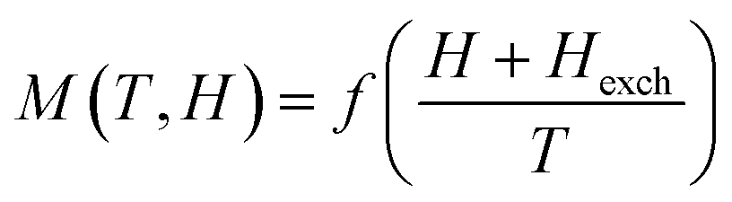 , we may obtain the relation:
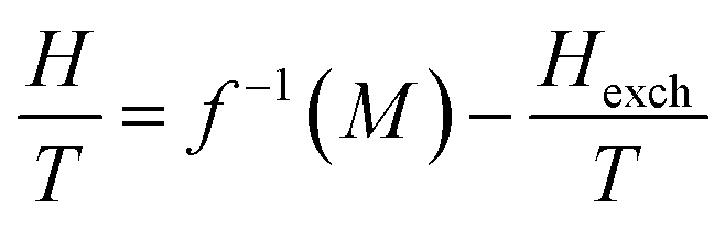 | (11) |
Then, ΔSM between two magnetic fields H1 → H2 can be estimated theoretically as follows:31
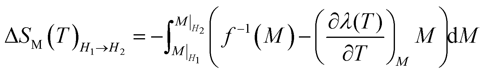 | (12) |
From the M(H, T) curves evaluated at constant values of magnetization M with a step of 2 emu g−1, the evolution of  as a function of
 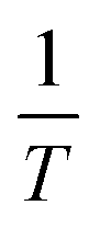 was plotted in Fig. 5(a). A linear behavior of the isomagnetic curves of
 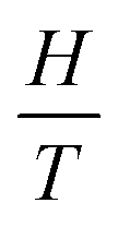 versus
  is observed. The lines gradually shift to larger values of the temperature. It is worth studying the Hexch to sort out the value of the mean-field exchange parameter λ. From eqn (11), the slopes of
  vs.
vs.  give the Hexch. Then, Hexch versus M was plotted in Fig. 5(b). Knowing that magnetization is an odd function of the exchange magnetic field:32
| Hexch = λ1M + λ3M3 | (13) |
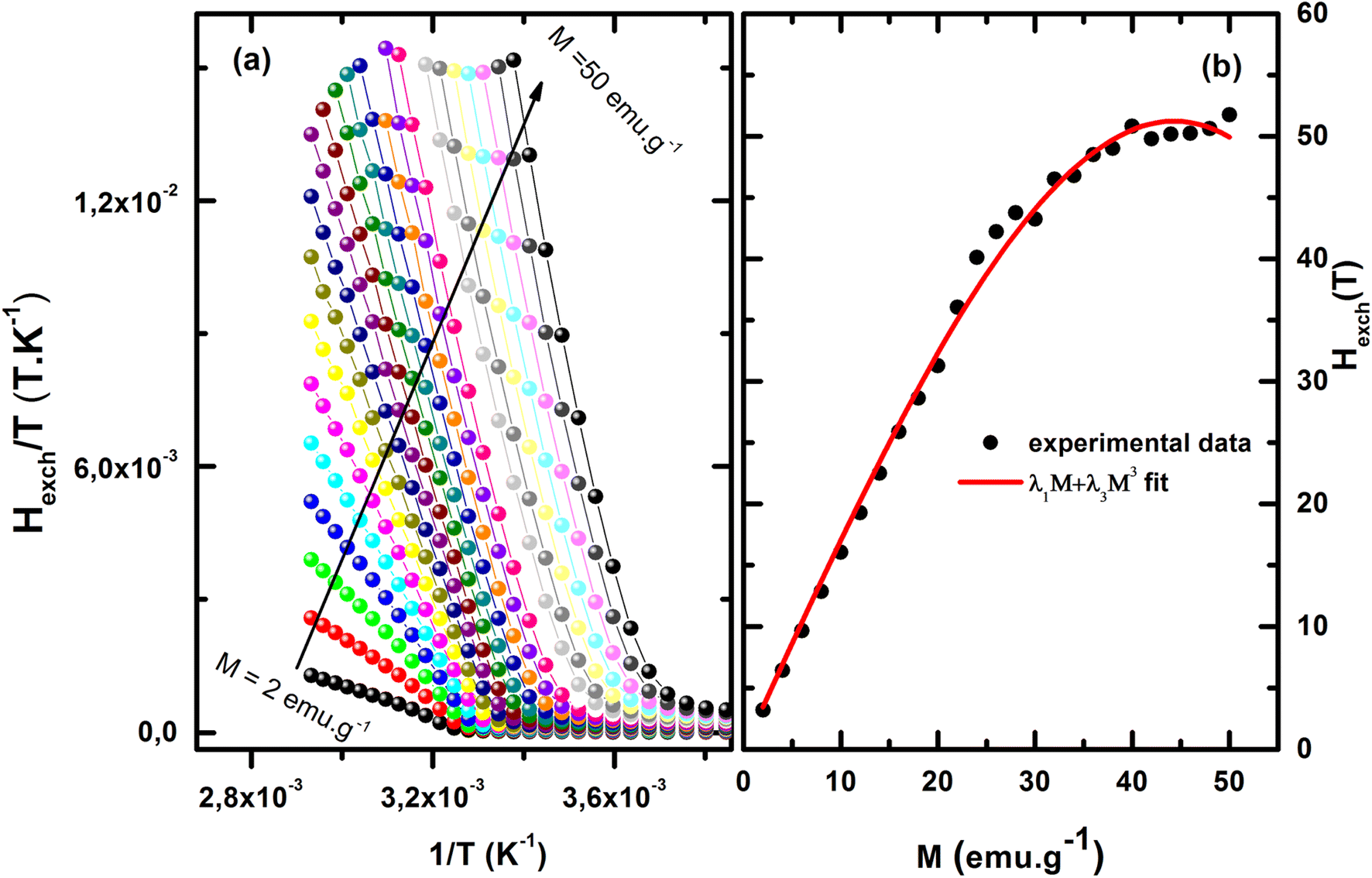 | ||
Fig. 5 (a) Evolution of  vs. vs.  with 2 emu g−1 step plot (b) fitting Hexch vs. M. with 2 emu g−1 step plot (b) fitting Hexch vs. M. | ||
Then, Hexch as a function of M in Fig. 5(b) was fitted by eqn (13). A very low dependence on M3 was noted (λ3 = −0.0003 (T emu−1 g)3). One can consider Hexch = λ1M ≈ λM, with λ1 = 1.73 T emu−1 g.
For La0.75Ca0.1Na0.15MnO3 manganite, using the Hund rules in ref. 30, J = g = 2. The saturation magnetization is given by fitting M(H, T) vs.  with eqn (10) (not shown here) and its value is found to be M0 = 103.9 emu g−1.
Adding parameters λ, J, g and M0 to eqn (10) enables the generation of M(H, T) curves (red lines) which are plotted in in Fig. 6(a) with experimental M(H, T) data (black symbols). A good agreement between the calculated and the experimental plots of M(H, T) was found.
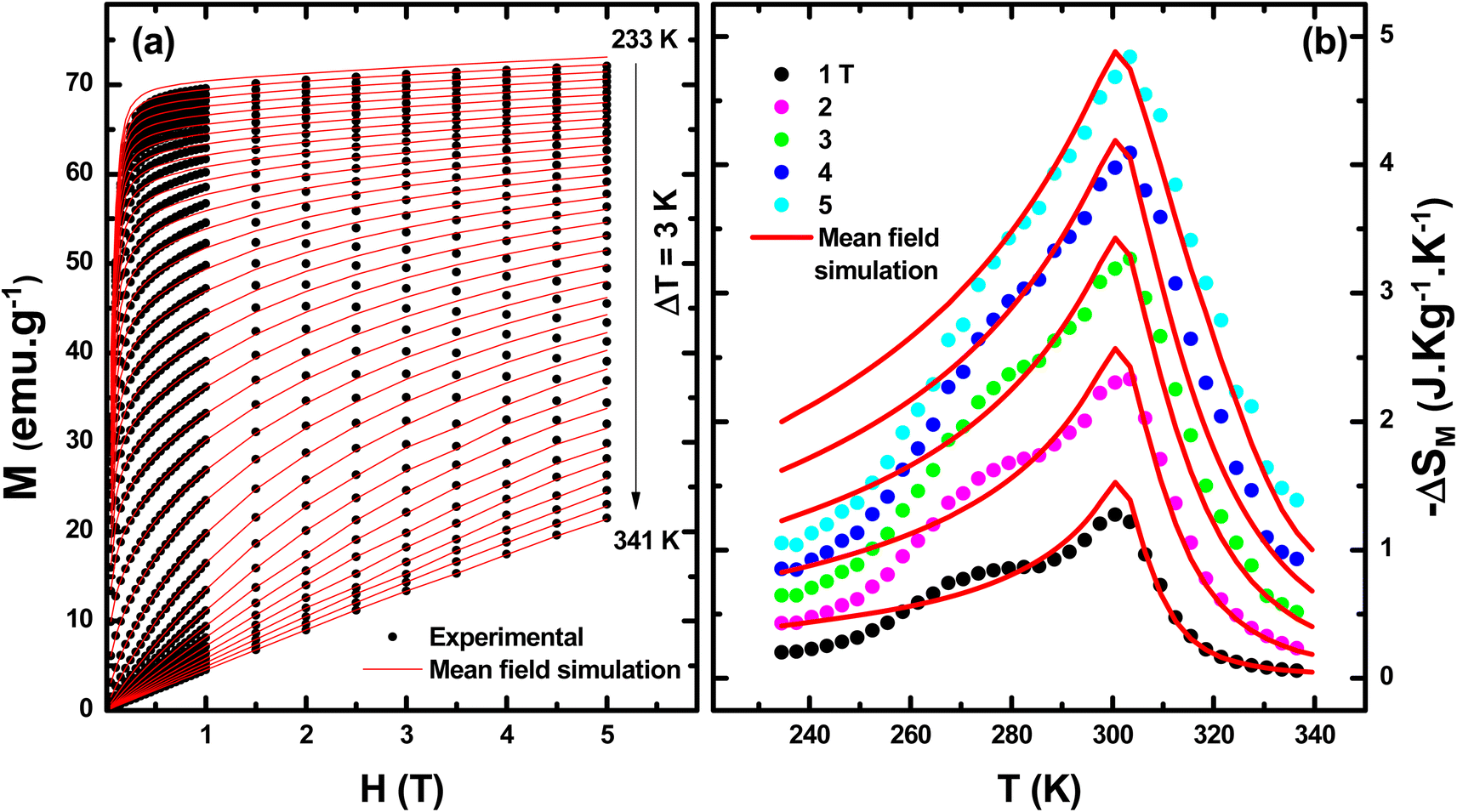 | ||
| Fig. 6 The experimental (symbols) and the simulated (red lines) curves of (a) M vs. H and (b) −ΔSM vs. T using the MFM. | ||
Fig. 6(b) shows the comparison between the −ΔSM curves using the MFM (red lines) from exploiting eqn (12) and the related experimental data (solid symbols) by using Maxwell's relation. The entropy results show a good agreement between simulated and experimental −ΔSM curves in the PM region but some notable discrepancies, especially in the FM range. These discrepancies may be associated with the high spontaneous magnetization in the FM area; the phase transition is far from the area of interest. In fact, this MS(T) obeys eqn (3) for a temperature range far from the transition where the ANE is not valid. When integrating eqn (2), MS(T) has been eliminated. But eqn (12) does not mention MS(T). This could be explained by the fact that the MFM is not able to accurately describe the magnetization and magnetic entropy in these temperature ranges (far from TC).33 In addition, some deviations of the simulated entropy results near TC may be associated to the fact that the MFM does not consider fluctuations and disorder effects (chemical and structural inhomogeneity) near TC.34
3 Conclusion
In conclusion, three models were exploited to investigate the MCE of La0.75Ca0.1Na0.15MnO3 (LCNMO) manganite. The ANE was analyzed to determine the critical exponents of the LCNMO magnetic system. The deduced critical exponents are found to be as: β = 0.48 and γ = 1. A close relationship between these estimated critical exponents and those identified by the Mean Field Model (MFM) with β = 0.5 and γ = 1. An excellent agreement exists between the simulated and the experimental curves of the isothermal magnetization M(H, T) and the magnetic entropy change −ΔSM(T) curves using the ANE and the Landau model near the FM–PM transition but in a short temperature range. Considering that the MFM may be adequate to analyze the MCE in LCNMO magnetic system, a good correlation was found between the M(H, T) and −ΔSM(T) curves generated by the MFM and the corresponding experimental data. The results of this MFM scaling method are very promising for a SO magnetic system. Moreover, it is interesting to emphasize that this analysis is global, in the sense that it encompasses the consistency of the whole range magnetization data.Data availability
The datasets generated or analysed during the current study are available from the corresponding author on reasonable request.Author contributions
The manuscript was written with the contributions of all authors. SB contributed to preparing experimental data. MH contributed to calculations. SS and ME contributed to editing of the manuscript. MAA and HB contributed to reviewing and editing of the manuscript. JD contributed to review of the manuscript and supervising.Conflicts of interest
There are no conflicts to declare.Acknowledgements
The authors extend their appreciation to the Deanship of Scientific Research at King Khalid University for funding this work through large group Research Project under grant number RGP2/110/44.References
- Z. Ma, P. Xu, J. Ying, Y. Zhang and L. Li, Acta Mater., 2023, 247, 11875 CrossRef.
- Y. Zhang, J. Zhu, S. Li, Z. Zhang, J. Wang and Z. Ren, Sci. China Mater., 2022, 65, 1345–1352 CrossRef CAS.
- Y. Zhang, Y. Tian, Z. Zhang, Y. Jia, B. Zhang, M. Jiang, J. Wang and Z. Ren, Acta Mater., 2022, 226, 117669 CrossRef CAS.
- D. Guo, L. M. Moreno-Ramírez, J. Law, Y. Zhang and V. Franco, Sci. China Mater., 2023, 66, 249–256 CrossRef CAS.
- P. Xu, L. Hu, Z. Zhang, H. Wang and L. Li, Acta Mater., 2022, 236, 118114 CrossRef CAS.
- Y. Zhang, P. Xu, J. Zhu, S. Yan, J. Zhang and L. Li, Mater. Today Phys., 2023, 32, 101031 CrossRef CAS.
- L. Li and M. Yan, J. Mater. Sci. Technol., 2023, 136, 1–12 CrossRef.
- S. Bouzidi, M. A. Gdaiem, J. Dhahri and E. K. Hlil, RSC Adv., 2019, 9, 65–76 RSC.
- A. S. Erchidi Elyacoubi, R. Masrour and A. Jabar, Solid State Commun., 2018, 271, 39–43 CrossRef CAS.
- N. H. van Dijk, J. Magn. Magn. Mater., 2021, 529, 167871 CrossRef CAS.
- M. Hsini, S. Hcini and S. Zemni, J. Magn. Magn. Mater., 2018, 466, 368–375 CrossRef CAS.
- M. Hsini, S. Hcini and S. Zemni, Eur. Phys. J. Plus, 2019, 134, 588 CrossRef CAS.
- A. Fujita and K. Fukamichi, IEEE Trans. Magn., 2005, 41, 3490–3492 CAS.
- V. S. Amaral, J. P. Araújo, Yu. G. Pogorelov, P. B. Tavares, J. B. Sousa and J. M. Vieira, J. Magn. Magn. Mater., 2002, 242–245, 655–658 CrossRef CAS.
- V. S. Amaral, et al., J. Appl. Phys., 2003, 93, 7646 CrossRef CAS.
- A. Arrott and J. E. Noakes, Phys. Rev. Lett., 1967, 19, 786 CrossRef CAS.
- V. Franco and A. Conde, Int. J. Refrig., 2010, 33, 465 CrossRef CAS.
- M. E. Fisher, Rep. Prog. Phys., 1967, 30, 615 CrossRef CAS.
- V. Franco, J. S. Blazquez and A. Conde, Appl. Phys. Lett., 2006, 89, 222512 CrossRef.
- V. Franco, A. Conde, J. M. Romero-Enrique and J. S. Blazquez, J. Phys.: Condens. Matter, 2008, 20, 285207 CrossRef.
- B. Widom, J. Chem. Phys., 1965, 43, 3898 CrossRef.
- A. Aharoni, Introduction to the Theory of Ferromagnetism, Clarendon Press, Oxford, 1996, ch. 4 Search PubMed.
- A. K. Pramanik and A. Banerjee, Phys. Rev. B: Condens. Matter Mater. Phys., 2009, 79, 214426 CrossRef.
- C. Romero-Muniz, J. J. Ipus, J. S. Blazquez, V. Franco and A. Conde, Appl. Phys. Lett., 2014, 104, 252405 CrossRef.
- V. S. Amaral and J. S. Amaral, J. Magn. Magn. Mater., 2004, 272–276, 2104–2105 CrossRef CAS.
- Q. Y. Dong, H. W. Zhang, J. L. Shen, J. R. Sun and B. G. Shen, J. Magn. Magn. Mater., 2007, 319, 56 CrossRef CAS.
- L. Zhang, J. Fan and Y. Zhang, Mod. Phys. Lett. B, 2014, 28, 1450059 CrossRef.
- J. Coey, Magnetism and Magnetic Materials, Cambridge University Press, Cambridge, 2009 Search PubMed.
- J. A. Gonzalo, Effective Field Approach to Phase Transitions and Some Applications to Ferroelectrics, World Scientific, Singapore, 2006 Search PubMed.
- C. Kittel, Introduction to Solid State Physics, John Wiley and Sons, New York, 7th edn, 1996 Search PubMed.
- J. S. Amaral, N. J. O. Silva and V. S. Amaral, Appl. Phys. Lett., 2007, 91, 172503 CrossRef.
- S. B. Ogale, R. Shreekala, R. Bathe, S. K. Date, S. I. Patil, B. Hannoyer, F. Petit and G. Marest, Phys. Rev. B: Condens. Matter Mater. Phys., 1998, 57, 7841 CrossRef CAS.
- B. Mohamed, F. Allab, C. Dupuis, D. Fruchart, D. Gignoux, et al., Analysis and modeling of magnetocaloric effect near magnetic phase transition temperature, in Second IIF-IIR International Conference on Magnetic Refrigeration at Room Temperature, Portoroz, Slovenia, 2007 Search PubMed.
- J. S. Amaral, P. B. Tavares, M. S. Reis, J. P. Araújo, T. M. Mendonça, V. S. Amaral and J. M. Vieira, J. Non-Cryst. Solids, 2008, 354, 5301–5303 CrossRef CAS.
| This journal is © The Royal Society of Chemistry 2023 |