Electrical and mechanical properties of self-supported hydroxypropyl methylcellulose–polyaniline conducting films

Abstract

The purpose of this work was to develop a simple method to produce self-supported films composed of hydroxypropyl methylcellulose (HPMC) and polyaniline (PANI) by the direct mixture of aqueous dispersions of both polymers with subsequent drying. The addition of HPMC, a cellulose derivative with an excellent film-forming capacity, was fundamental to overcoming the poor processability of PANI, which impairs its use in many technological applications. All films showed conductivity in the order of 10⁻² to 10⁻³ S cm⁻¹, which is in the range for metals or semiconductors. The typical electroactivity of PANI was also maintained in the hybrid films. The thermal stability and the mechanical properties of the pristine PANI were also improved with the addition of HPMC. Cellulose-containing conducting polymers can be considered a material of the future, with possible applications in several areas, such as smart wallpapers, e-papers, and sensors.

---

Introduction

Polyaniline (PANI) is one of the most studied conducting polymers due to its ease of synthesis, low cost, reversible redox properties, and thermal and chemical stabilities.¹ Owing to its attractive features, PANI has been applied in various fields such as sensors, anticorrosion and antistatic coatings, and electrochromic displays.^2–9 Despite these advantages, polyaniline is relatively hard to process due to its insolubility in the majority of usual solvents and its poor mechanical strength. In addition, it cannot be easily cast into films, and membranes, molded into different shapes, or extruded into fibers, significantly impairing its use in many technological applications.¹⁰ To overcome these limitations, the combination of this conducting polymer with other polymeric matrices with superior mechanical properties has been proposed. Among these polymers, hydroxypropyl methylcellulose (HPMC) is one of the most attractive, since it is a water-soluble cellulose derivative and a good film-forming material with several potential applications.^11,12 The incompatibility between these polymers, due to the solubility differences, is a drawback to be overcome, and the search for a preparation method that will promote the intimate combination between the components is needed.¹³ Only a few recent studies have explored the preparation of conductive composite based on HPMC and PANI films. In 2020, Kim and co-workers have fabricated a flexible composite based on PANI and cellulose fabrics with electrical conductivity in the order of 10⁻² S cm⁻¹.¹⁴ In 2017, Hussin and colleagues developed a procedure to produce aqueous PANI-cellulose derivatives dispersions through the polymerization of aniline monomer in cellulose solution initiated by ammonium persulphate.¹³ Later, these investigators used the PANI-HPMC composite as a chemical sensor for detecting hydrazine in aqueous effluents through the electrical conductivity values variation of the dispersion.¹⁵

This study aims to prepare conductive films based on HPMC and polyaniline (Fig. 1) using a simple procedure. To produce homogenous films, it was used a water-soluble polyaniline dispersion. Using this procedure, the conductive polymer was well-dispersed in the cellulose matrix, which is important for the movement of electrons occurs without interruption and the maintenance of the electrical properties.^16,17 The chemical and physical structures, electrical conductivity, and mechanical properties of the conductive cellulose film were evaluated. The excellent film-forming capacity of HPMC was fundamental to overcoming the poor processability of PANI, which impairs its use in many technological applications.

Fig. 1 PANI and HPMC structures.

Experimental

Materials and methods

Hydroxypropyl methylcellulose (HPMC) (Vivapur K4M, J. Rettenmaier & Söhne GmbH + Co KG) was used as purchased. Aqueous solutions of HPMC (2% w/w) were prepared by adding the required amount of polymer to distilled water. This solution was denominated HPMC_H₂O. Aniline (Aldrich, 99%) was distilled before use. Polyvinylpyrrolidone (PVP) (Aldrich, average molecular weight of 360 000) and ammonium persulphate (Aldrich, 98%) were used as purchased.

Preparation of the polyaniline aqueous dispersion

This dispersion was synthesized following a procedure described in the literature.¹⁸ Firstly, aniline hydrochloride was prepared by mixing aniline (85 mmol) and concentrated hydrochloric acid (85 mmol). After the removal of the solvent under reduced pressure using a rotary evaporator (10 mmHg at 60 °C), a white solid was obtained (melting point: 196–198 °C).¹⁹ Then, an aqueous solution of ammonium persulphate (5.71 g in 50 mL deionized water; 25 mmol) was prepared (solution A). Aniline hydrochloride (2.59 mg; 20 mmol) was dissolved in 50 mL of an aqueous solution of PVP (40 g L⁻¹) (solution B). Solution A and B were mixed at room temperature for 10 minutes and then left at rest to polymerize. The polymerization was completed in several minutes (30 minutes). The dispersion was exhaustively dialyzed against 0.2 mol L⁻¹ HCl to remove ammonium sulfate resulting from the decomposition of ammonium persulphate and residual monomer. Dialysis tubing cellulose membrane with a typical molecular weight cut-off of 14 000 was used. A green dispersion was obtained (Fig. S1 – ESI†).

Fabrication of HPMC-PANI films

HPMC_H₂O solution was mixed with different volumes of the PANI dispersion at room temperature for 15 minutes. Films with distinct amounts of HPMC (0, 5, 10, 20, 30, 40 w/w%) were prepared. The amounts used in the preparations are indicated in Table 1. The resulting solutions were transferred into polystyrene Petri dishes (diameter = 8.5 cm) and dried at 60 °C overnight. These films were denoted as PANI_x%HPMC, where x is the mass percentage of HPMC. All calculations are shown in Note 1 in the ESI.† An illustration of this preparation procedure is shown in Fig. S1 (ESI†).

Table 1 Amounts of components used in the PANI_x%HPMC films^a

Sample	Mass of HPMC solution^b (g)	HPMC mass (mg)	Volume of PANI dispersion (mL)	PANI mass (mg)	PVP mass (g)	wt% of HPMC	wt% of PANI	wt% of PVP
a All calculations are shown in Note 1 (ESI).b Aqueous solutions of HPMC (2% w/w).
PANI	0	0	19.20	416	384	0	52.0	48.0
PANI_5%HPMC	2.00	40	18.20	395	365	5	49.4	45.6
PANI_10%HPMC	4.00	80	17.30	374	346	10	46.8	43.2
PANI_20%HPMC	8.00	160	15.40	333	307	20	41.6	38.4
PANI_30%HPMC	12.00	240	13.40	290	270	30	36.3	33.7
PANI_40%HPMC	16.00	320	11.50	250	230	40	31.3	28.7

---

Characterization

Thermal analyses (TGA) were carried out on DTG-60 SHIMADZU equipment, using an aluminium crucible, a heating rate of 5 °C min⁻¹, and under a synthetic air flow of 100 mL min⁻¹ in a temperature range of 30–900 °C.

Dynamic mechanical analysis (DMA) was performed in a DMA Q800-TA instrument using an air atmosphere with bending deformation at a heating rate of 5 °C min⁻¹ from 30 to 300 °C. The tests were carried out with a fixed frequency of 1 Hz, 1 N applied pre-force, and an oscillation amplitude of 25 μm. The films were cut into 6 mm × 40 mm.

For the attenuated reflectance measurements, a horizontal ATR sampling accessory (ATR-8200HA) equipped with a ZnSe cell was employed. All spectra were carried out using a Shimadzuprestige-21 spectrometer in the range of 4000–700 cm⁻¹ with a 4 cm⁻¹ resolution.

Electronic absorption spectra were recorded in an Ocean Optics spectrophotometer model USB 4000. The films were vertically positioned (perpendicular to the light beam) in a homemade sample holder. The spectra of each film were measured using the non-irradiated film itself as a blank to have the light scattering of the films compensated.

X-ray diffractograms (XRD) were recorded in a BRUKER D8 Advance lab diffractometer using the CuKα radiation (λ = 1.54 Å) from a generator operating at 40 keV and 40 mA as the applied voltage and current, respectively.

MALDI-TOF measurements were performed with a Bruker UltrafleXtreme in the reflector acquisition operation mode. The spectrum was recorded using the PANI sample solution in the presence of the matrix 2,5-dihydroxybenzonic acid (DHB).

Scanning electron microscopy (SEM) images of the films were registered using a JSM-6610 microscope by JEOL, using secondary electron detection mode with carbon-coated samples.

Cyclic voltammetry experiments were performed in a potentiostat (METROHM AUTOLAB model 302 N) using a single-compartment electrochemical cell. A carbon glass electrode (Metrohm, geometric area = 0.0314 cm²) was used as a working electrode, a Pt wire as a counter electrode, and an Ag/AgCl (KCl 3 mol L⁻¹) as a reference electrode. These measurements were carried out in different potential windows ranging from −0.2 V to 0.8 V with a scan rate of 100 mV s⁻¹ in 1.0 M HCl aqueous solution. The working electrode was modified via drop-casting of four sequential depositions of 10 μL of the dispersion followed by drying at 40 °C.

Zeta potentials of the dispersions were measured in disposable folded capillary cells (DTS1070) in triplicate in a Zetasizer Nano ZS from Malvern.

Tensile strength (MPa) and elongation at break (%) were measured using a Brookfield CT3 texture analyser with a dual grip assembly (TA3/100). The preload force was set to 0.07 N and all tests were performed at a strain rate of 0.05 mm s⁻¹ until the films rupture. The samples were cut into rectangle strips (100 mm × 25.4 mm) and fixed on the grips of the stretching unit. The tensile strength was estimated by dividing the maximum load by the cross-sectional area of the film (thickness × width) while the elongation at break was obtained as the percentage of extension at the moment of rupture.

The electrical conductivity measurements were performed in triplicate using a four-point method with FPP200 equipment at room temperature and 55% of humidity.

Results and discussion

The aqueous dispersion of polyaniline was prepared by the oxidation of aniline by sulfate persulfate using polyvinylpyrrolidone as a stabilizer, following a well-established procedure described in the literature.¹⁸ In the absence of PVP, the polyaniline chains would aggregate and precipitate from the solution and a water-stable dispersion would not be obtained. As described in the literature PVP adsorbs on the PANI particle surface, inhibiting aggregation.²⁰ The crude product was dialyzed to remove any reaction byproducts and low molecular weight impurities. A green dispersion was obtained, which is the typical color of the PANI in the emeraldine salt oxidation state (Fig. S1 – ESI†). The absorption spectrum (Fig. 2) has a broad band located between 300–450 nm which is characteristic of π–π* and polaron–π* transitions and another between 600 to 800 nm assigned by the π–polaron transition. These features confirmed the formation of emeraldine salt form.²¹ The spectra collected from this sample each week for 2 months were identical, indicating that it is stable with time. The zeta potential of the PANI dispersion was 0.64 ± 0.20 mV, suggesting that PVP, a neutral polymer, is responsible for the steric stabilization of this sample.²² MALDI-TOF was used to provide the molecular weight of synthesized PANI (Fig. S2 – ESI†). The spectrum revealed the presence of a complex mixture. Peaks are ranging from m/z = 600 to 2500 that can be tentatively assigned to a polymer chain with 26 repeating units (considering the monomer unit of PANI (C₆NH₅) = 93). The complexity occurs because oligomers and polymers show different peak clusters, corresponding to several redox states and different end groups. The detection of longer polymers could not be identified since they can be entrapped inside the PVP with high molecular weight (MW = 360 000) and therefore, it is not accessible for detection.²³

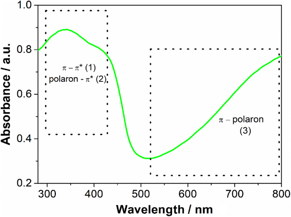Fig. 2 UV-Vis absorbance spectra of polyaniline dispersion.

Hydroxypropyl methylcellulose-PANI films were prepared by simple mixing of the aqueous solutions of PANI and HPMC, followed by drying. The films were self-supported and showed green color and they seem homogeneous in appearance to the naked eye (Fig. 3). It is worth mentioning that on closer observation obtained in an electronic microscope (MEV), this homogeneity is also revealed (Fig. S3 – ESI†). PANI_40%HPMC has similar morphology to HPMC and PANI samples (Fig. S3A and B†) and its surface is smooth and without pores.

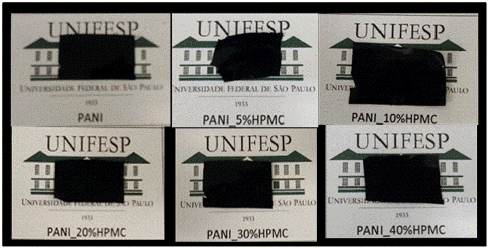Fig. 3 Photos of the HPMC-PANI films.

Aiming to apply these films as conductive materials, the electrical conductivities at room temperature in three different places of the sample were measured (Table 2). The measurements were quite similar, indicating that the samples were homogeneous. The incorporation of PANI as a conductive loading into the HPMC, which is an insulator material, leads to an increase in electrical conductivities. All films can be classified as conductive paper because the conductivity is around 10⁻³ cm⁻¹, which is in the range of metals or semiconductors.²⁴ Independently of the HPMC loading, the electrical conductivity values of the films are in the same order of magnitude. One explanation is that the conductive loading (PANI) is homogeneously distributed in the HPMC membrane.

Table 2 Electrical conductivity values of the films

Sample	Electrical conductivity^a (S cm^−1)
a Arithmetic average.
HPMC	Insulating material
PANI	17 × 10^−3 ± 5.7 × 10^−4
PANI_5%HPMC	11 × 10^−3 ± 7.3 × 10^−4
PANI_10%HPMC	9.1 × 10^−3 ± 1.9 × 10^−4
PANI_20%HPMC	7.6 × 10^−3 ± 2.9 × 10^−5
PANI_30%HPMC	6.3 × 10^−3 ± 1.6 × 10^−3
PANI_40%HPMC	5.4 × 10^−3 ± 6.9 × 10^−4

---

Given the conductivity results, in further characterizations (FTIR, DRS, TGA, DMA, tensile tests), only the samples with the lowest and highest amount of HPMC were analyzed.

PANI film (Fig. 4A) reveals bands at 821, 1157, 1491, 1582–1609 cm⁻¹ (highlighted with green rectangles) attributed to C–H (the first three ones) and C=C benzenoid and quinoid ring vibrations. The band located at 1350 cm⁻¹ (pointed out with a black arrow) has been assigned to the vibration mode of the C–N⁺ structure in the emeraldine salt form of polyaniline.¹⁸ In addition, the typical bands of PVP are seen at 1291, 1424 and 1656 cm⁻¹ (highlighted with magenta rectangles) designated to the C–N stretching, C–H bending, and C=O stretching.²⁵ The FTIR spectrum of the pristine PVP film was shown in the inset of Fig. 4 for comparison. The carbonyl stretching band observed in the PVP at 1660 cm⁻¹ suffers a slight change in the PANI sample, suggesting the interaction of this functional group with the N–H bonds (e.g.) present in the PANI structure, as previously reported in the literature.²⁶

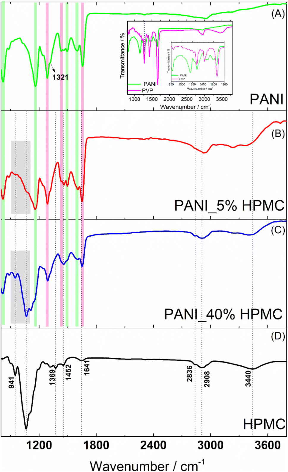Fig. 4 FTIR spectra of PANI (green), PANI_5%HPMC (red) and PANI_40%HPMC (blue) and HPMC (black).

FTIR spectrum of HPMC film (Fig. 4D) exhibits absorptions related to the C–O axial deformation around 1060 and 941 cm⁻¹ and C–H stretching bands in the range of 2800–2900 cm⁻¹. Bands at wavenumbers around 1369 and 1452 cm⁻¹ are assigned to the angular deformation of C–H bonds within –(CH₂)_n– chains. The bands close to 1639 and 3455 cm⁻¹ are related to the angular and axial deformations of the residual hydroxyl groups or adsorbed water, present in the HPMC film, respectively.²⁷

The spectra of the PANI films containing 5 and 40% HPMC (Fig. 4B and C) contain the characteristic vibrations of PANI and HPMC discussed previously. As expected, the sample PANI_5%HPMC is especially like pure PANI (Fig. 4A), since this is the majority component, while in the sample PANI_40%HPMC the cellulose vibrations seemed more evidently. The minor differences can be attributed to the interaction of HPMC and PANI as shown in Fig. S4 (ESI†).

UV-vis diffuse reflectance spectra of the HPMC, PANI, and PANI_x%HPMC samples are shown in Fig. 5A. In comparison to the pristine HPMC membrane which shows a relatively high diffuse reflection in the visible range, the PANI_x%HPMC films independently of the HPCM loading, exhibit a quite low reflection over UV and visible range, as the neat PANI sample, due to great light absorption of this polymer as discussed before. The band gaps of the PANI_x%HPMC films were estimated by extrapolating the tangent line in the plot of (F(R)hυ)² against energy (Fig. 5B). The band gap of PANI is following some previous works.^28,29 The band gap values increase with HPMC loading. This might result from the weakening of the electronic properties of the hybrid membrane due to the insulating nature of HPMC. Band gaps values for the PANI_x%HPMC samples are close to each other and coherent with conductivity data.

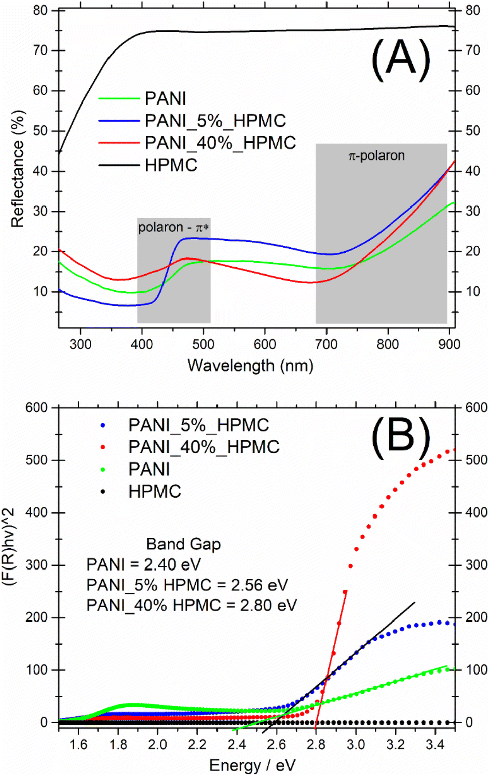Fig. 5 (A) UV-vis diffuse reflectance spectra of PANI (green), PANI_5%HPMC (red) and PANI_40%HPMC (blue) and HPMC (black) (B) F(R) versus E.

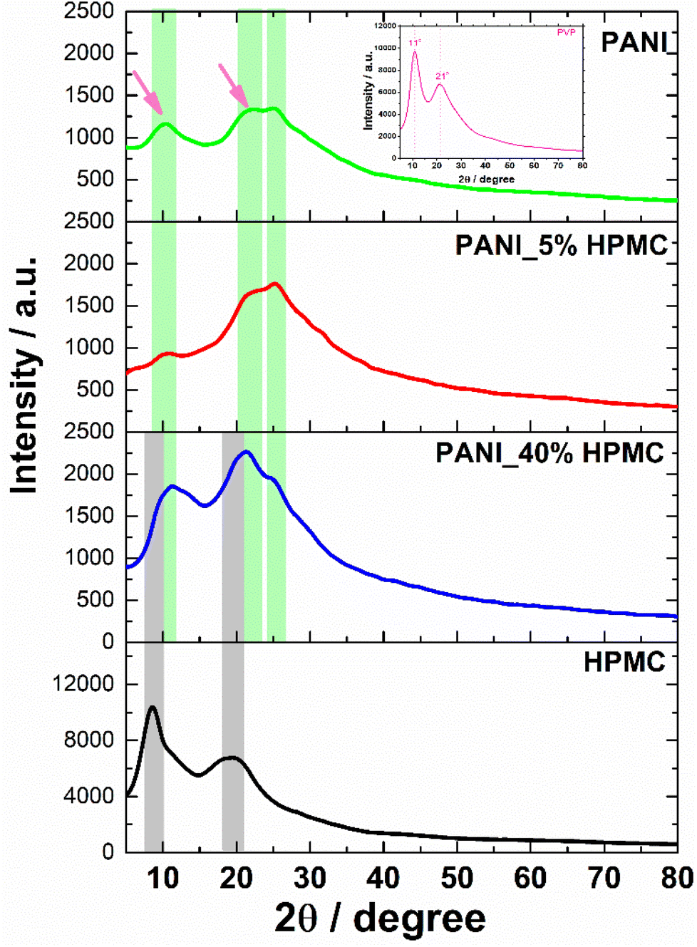
HPMC membrane shows two broad halos in the range 2θ = 9–10° and 2θ = 20–21° seen in Fig. 6.³⁰ In turn, the PANI membrane has two weak diffraction halos in 2θ = 11° and 22° (pointed with magenta arrows), attributed to PVP³¹ (inset in Fig. 6) and also a shoulder at 2θ = 25°, typical of PANI.³² PANI_5% HPMC diffractogram is similar to the PANI sample, while PANI_40% HPMC sample contains HPMC and PANI diffractions overlapped.³³ These data have shown that the films PANI_x% HPMC films are amorphous.

Fig. 6 DRX of PANI (green), PANI_5%HPMC (red) and PANI_40%HPMC (blue) and HPMC (black).

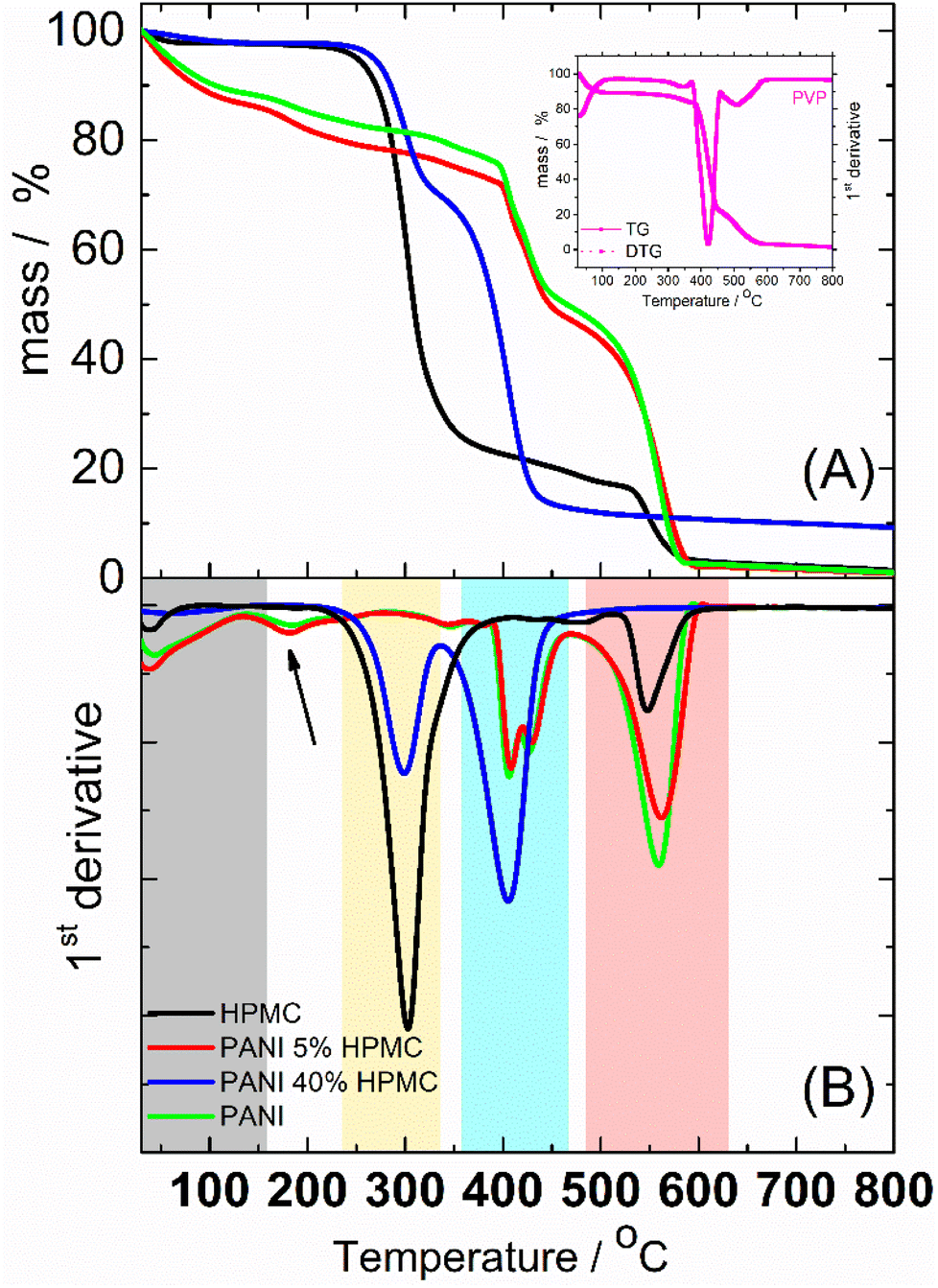
Thermogravimetric (TG) (Fig. 7A) analyses were implemented to study the thermal behavior of the films. The thermal decomposition of HPMC could be roughly divided into 3 stages, as seen in the first derivative curve (DTG) (Fig. 7B). The small weight loss from room temperature to 150 °C was attributed to the elimination of absorbed water. The second stage taking place in the temperature range of 150–450 °C (DTG peak at ca. 300 °C) was designated as the main pyrolysis.³⁴ At higher temperatures (DTG peak at ca. 550 °C) took a further decarboxylation and complete carbonization. PANI and PANI_5%HPMC thermograms are similar and show four main steps of weight loss. The first one begins at room temperature and continues until 150 °C (gray rectangle) due to the loss of water³⁵ and oligomers.³⁶ The mass loss in the temperature range of ∼150–350 °C (pointed with a black arrow) is due mainly to the elimination of PANI dopant. The two-step weight loss seen in DTG at around 420 °C (blue rectangle) is a result of the PVP³⁷ degradation present in both samples. After 500 °C (rose rectangle) occurs the degradation of the PANI backbone³⁵ and HPMC in the case of the PANI_5%HPMC sample. PANI_40%HPMC has a thermal behavior like HPMC from 30 °C till 350 °C, however at higher temperatures seems that the decomposition of PVP, PANI, and HPMC occurs in one step observed at 410 °C, indicating good miscibility of all components. The addition of 40 wt% of HPMC increases the thermal stability of the PANI film.

Fig. 7 (A) TG curves of HPMC, PANI, PANI_5%HPMC and PANI_40%HPMC (B) First derivative.

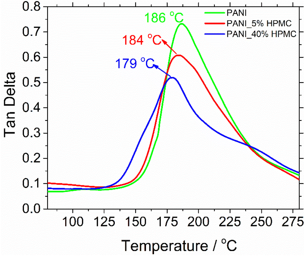
The glass transition temperatures (T_g) were measured using dynamic mechanical analysis (DMA). Although there are several thermal techniques available to make T_g measurements, by far DMA is the most sensitive technique.³⁸ T_g has been obtained respectively at the maximum tan δ peak curves (Fig. 8). The glass transition temperature of neat PANI is seen at 186 °C. This transition can be understood as the thermal motion of individual chain segments along the polymer backbone. This temperature dropped to 179 °C when HPMC is added.²⁹ Such an effect can be attributed to the presence of cellulose derivative in the PANI matrix, which increases the mobility of polymer chains and so as a result, the transition happened at the lower temperatures.

Fig. 8 Tangent delta curves of PANI, PANI_5%HPMC, and PANI_40%HPMC.

The effect of HPMC on the mechanical properties of the neat polyaniline film was evaluated by tensile tests. The stress–strain curves of the films are illustrated in Fig. S5 (ESI†). From these data, the tensile strength (TS) and elongation at break (E) were calculated (Table 3) and they are shown in Fig. 9. Tensile strength at break measures the maximum stress that a specimen can withstand while being stretched before breaking, while elongation at break measures how much bending and shaping a material can withstand without breaking. HPMC film has the highest tensile strength and elongation, in agreement with literature data.^39,40 On the other hand, PANI shows the lowest TS and elongation, indicating that this film exhibits a brittle character. As HPMC is added, independently of the percentage, TS and E% increase, indicating the films become more resistant. In addition, the elastic deformation of both samples containing HPCM is higher than that of the neat PANI film.

Table 3 Tensile strength and elongation of the PANI, PANI_x%HPMC, and HPMC films

Sample	Tensile strength/MPa	Elongation/%
HPMC	55.7 ± 3.16	0.167 ± 0.015
PANI	5.11 ± 0.42	0.018 ± 0.002
PANI_5%HPMC	9.16 ± 0.08	0.075 ± 0.003
PANI_40%HPMC	8.40 ± 0.24	0.101 ± 0.006

---

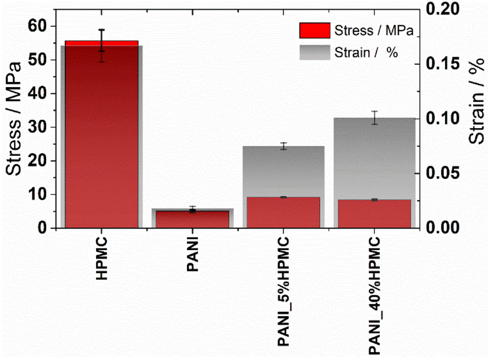Fig. 9 Tensile strength and elongation values of the HPMC, PANI, PANI_5%HPMC, and PANI_40%HPMC.

Cyclic voltammetry was used to monitor the electroactivity of polyaniline in the films (Fig. 10). PANI (green) and PANI_5%HPMC (red) voltammograms are quite similar, which is the typical response of the conducting polymer. Two redox processes are seen, the first anodic peak observed at 0.34 V, designated as P1, corresponds to the transformation of the leucoemeraldine form to the emeraldine form of polyaniline. The second one (P2) around 0.57 V corresponds to the transformation of the emeraldine form into the pernigraniline form of polyaniline.⁴¹ On the other hand, due to the higher loading of HPMC, an insulating polymer, the electroactivity response is decreased in the PANI_40%HPMC sample. The modified electrode (PANI_5%HPMC) was cycled during fifty cycles, and the peak shapes and the corresponding current values remained constant during successive cycles, suggesting excellent cycling stability (Fig. S6 – ESI†).

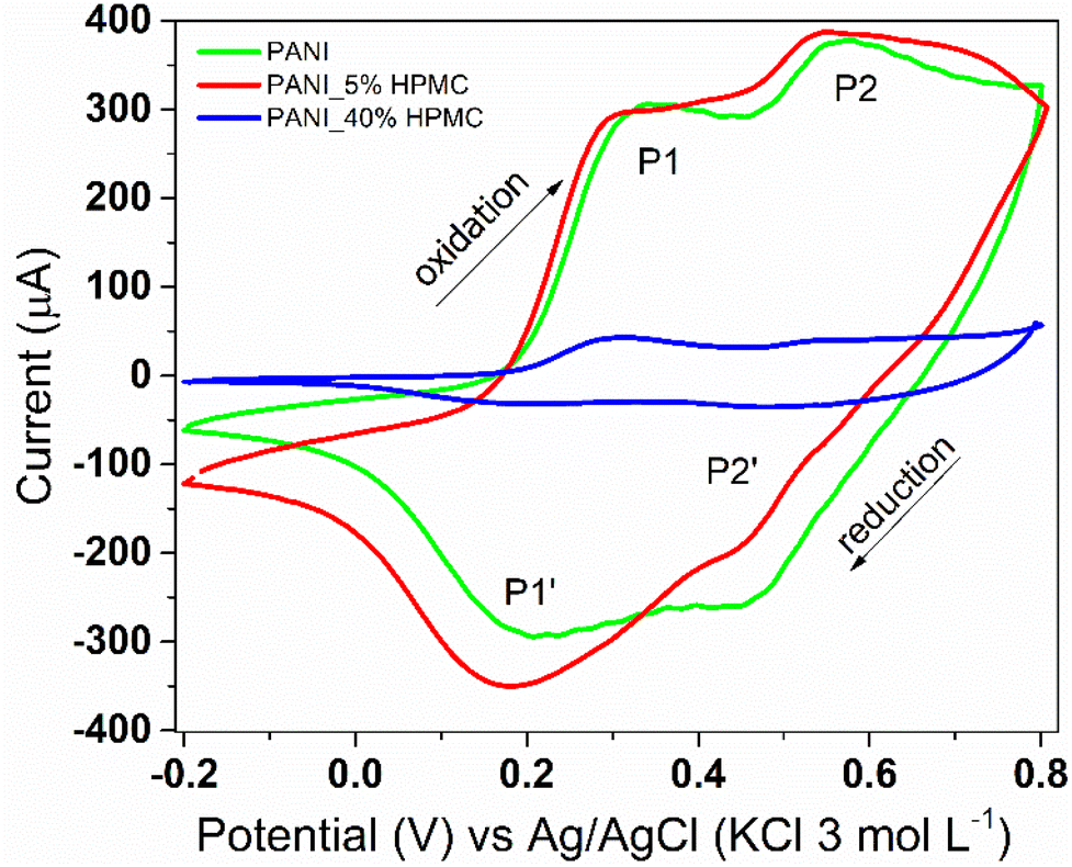Fig. 10 Cyclic voltammograms of PANI (green), PANI_5%HPMC (red) and PANI_40%HPMC (blue). Scan rate 100 mV s⁻¹ in 1.0 M HCl aqueous solution.

Conclusions

This work presented a remarkably simple method of preparing self-supported films based on PANI and HPMC. The use of an aqueous solution of PANI was the distinctive aspect of this preparation, which has permitted complete miscibility among the components. All hybrid films had electrical conductivity in the order of 10⁻² to 10⁻³ S cm⁻¹ and the typical electroactivity of the PANI, despite the insulating feature of HPMC. The addition of HPMC in the pristine PAN resulted in improved mechanical properties that can be seen through the tensile tests performed. Cellulose hybrid films with conducting polymer can open new horizons in the field of smart paper technology and can be used in developing flexible electrochemical sensors.

Author contributions

Study conception: Celso Molina and Fernanda Ferraz Camilo. Data collection and analysis: all authors. Supervision: Celso Molina and Fernanda Ferraz Camilo. First draft of the manuscript: all authors. All authors have read and approved the final manuscript.

Conflicts of interest

The authors declare that they have no known competing financial interests or personal relationships that could have appeared to influence the work reported in this paper.

Acknowledgements

This study was financed in part by the Coordenação de Aperfeiçoamento de Pessoal de Nível Superior – Brasil (CAPES) – Finance Code 001. Fernanda F. Camilo gratefully acknowledges the financial support from FAPESP (Grant Numbers 2018/20826-4 and 2021/08987-5) and CNPq scientific productivity fellowship (Grant Number: 310893/2021-6).

References

1. Z. A. Boeva and V. G. Sergeyev, Polym. Sci., Ser. C, 2014, 56, 144–153.
2. P. P. Deshpande, N. G. Jadhav, V. J. Gelling and D. Sazou, J. Coat. Technol. Res., 2014, 11, 473–494.
3. K. Hyodo, Electrochim. Acta, 1994, 39, 265–272.
4. G. A. Snook, P. Kao and A. S. Best, J. Power Sources, 2011, 196, 1–12.
5. X. Hong, Y. Liu, Y. Li, X. Wang, J. Fu and X. Wang, Polymers, 2020, 12, 331.
6. S. Mondal, U. Rana and S. Malik, Chem. Commun., 2015, 51, 12365–12368.
7. S. Mondal, U. Rana, P. Das and S. Malik, ACS Appl. Polym. Mater., 2019, 1, 1624–1633.
8. S. Mondal, U. Rana and S. Malik, ACS Appl. Mater. Interfaces, 2015, 7, 10457–10465.
9. S. Mondal and S. Malik, J. Power Sources, 2016, 328, 271–279.
10. A. Bhattacharya and A. De, Prog. Solid State Chem., 1996, 24, 141–181.
11. A. Fahs, M. Brogly, S. Bistac and M. Schmitt, Carbohydr. Polym., 2010, 80, 105–114.
12. M. Wrona, M. J. Cran, C. Nerín and S. W. Bigger, Carbohydr. Polym., 2017, 156, 108–117.
13. H. Hussin, S. N. Gan, S. Mohamad and S. W. Phang, Polym. Polym. Compos., 2017, 25, 515–520.
14. H. Kim, J.-Y. Yi, B.-G. Kim, J. E. Song, H.-J. Jeong and H. R. Kim, PLoS One, 2020, 15, e0233952.
15. H. Hussin, S.-N. Gan and S.-W. Phang, Polym. Bull., 2022, 79, 1843–1856.
16. M. S. Cho, S. Y. Park, J. Y. Hwang and H. J. Choi, Mater. Sci. Eng., C, 2004, 24, 15–18.
17. L. Liu and J. C. Grunlan, Adv. Funct. Mater., 2007, 17, 2343–2348.
18. J. Stejskal and I. Sapurina, Pure Appl. Chem., 2005, 77, 815–826.
19. A. Furst and R. E. Moore, J. Am. Chem. Soc., 1957, 79, 5492–5493.
20. S. Bongiovanni Abel, M. A. Molina, C. R. Rivarola, M. J. Kogan and C. A. Barbero, Nanotechnology, 2014, 25, 495602.
21. M. Trchová, I. Šeděnková, Z. Morávková and J. Stejskal, Polym. Degrad. Stab., 2014, 109, 27–32.
22. P. R. Somani, Mater. Chem. Phys., 2003, 77, 81–85.
23. E. Shim, J. Noro, A. Cavaco-Paulo, H. R. Kim and C. Silva, Front. Bioeng. Biotechnol., 2020, 8, 438.
24. F. M. Kelly, J. H. Johnston, T. Borrmann and M. J. Richardson, Eur. J. Inorg. Chem., 2007, 2007, 5571–5577.
25. K. M. Koczkur, S. Mourdikoudis, L. Polavarapu and S. E. Skrabalak, Dalton Trans., 2015, 44, 17883–17905.
26. R. da S. Oliveira, M. A. Bizeto and F. F. Camilo, Carbohydr. Polym., 2018, 199, 84–91.
27. H. S. Bhatti, S. Kumar, K. Singh and Kavita, J. Mater. Sci., 2013, 48, 5536–5542.
28. F. Usman, J. O. Dennis, K. C. Seong, A. Yousif Ahmed, F. Meriaudeau, O. B. Ayodele, A. R. Tobi, A. A. S. Rabih and A. Yar, Results Phys., 2019, 15, 102690.
29. A. A. M. Farag, A. Ashery and M. A. Rafea, Synth. Met., 2010, 160, 156–161.
30. G. Perfetti, T. Alphazan, W. J. Wildeboer and G. M. H. Meesters, J. Therm. Anal. Calorim., 2012, 109, 203–215.
31. D.-G. Yu, L.-M. Zhu, C. J. Branford-White, J.-H. Yang, X. Wang, Y. Li and W. Qian, Int. J. Nanomed., 2011, 6, 3271.
32. C. M. Correa, R. Faez, M. A. Bizeto and F. F. Camilo, RSC Adv., 2012, 2, 3088.
33. K. Lewandowska, Prog. Chem. Appl. Chitin Its Deriv., 2014, 19, 65–71.
34. R. Das, A. B. Panda and S. Pal, Cellulose, 2012, 19, 933–945.
35. N. Peřinka, M. Držková, M. Hajná, B. Jašúrek, P. Šulcová, T. Syrový, M. Kaplanová and J. Stejskal, J. Therm. Anal. Calorim., 2014, 116, 589–595.
36. X. Feng, Y. Zhang, Z. Yan, N. Chen, Y. Ma, X. Liu, X. Yang and W. Hou, J. Mater. Chem. A, 2013, 1, 9775.
37. P. Ghosh, A. Chakrabarti and S. K. Siddhanta, Eur. Polym. J., 1999, 35, 803–813.
38. S. Ebnesajjad, Surface Treatment of Materials for Adhesive Bonding, Elsevier, 2014.
39. C. Bilbao-Sainz, J. Bras, T. Williams, T. Sénechal and W. Orts, Carbohydr. Polym., 2011, 86, 1549–1557.
40. M.-J. Akhtar, M. Jacquot, M. Jamshidian, M. Imran, E. Arab-Tehrany and S. Desobry, Food Hydrocolloids, 2013, 31, 420–427.
41. P. R. Deshmukh, N. M. Shinde, S. V. Patil, R. N. Bulakhe and C. D. Lokhande, Chem. Eng. J., 2013, 223, 572–577.

---

Footnote

† Electronic supplementary information (ESI) available. See DOI: https://doi.org/10.1039/d3ra00916e

---