
 Open Access Article
 This Open Access Article is licensed under a Creative Commons Attribution-Non Commercial 3.0 Unported Licence
Desorption and ablation regimes in UV-MALDI: the critical fluence†
E. Alonso *a and
A. Peralta Condeb
*a and
A. Peralta Condeb
aPlasma novus – clean air solutions s.l, Department of Research and Development, Avda, de francisco vallés, no 8. 1a Planta, Oficina 7. Edificio Bioincubadora – Parque Tecnológico de Boecillo, Boecillo 47151, Valladolid, Spain. E-mail: eduardo.alonso@plasmanovus.com
bUniversidad Internacional de la Rioja, UNIR, Spain. E-mail: alvaro.peralta@unir.net; Web: https://www.unir.net
First published on 3rd January 2023
Abstract
Although MALDI is a widely used technique, there is so far no theoretical description able to reproduce some critical aspects of the experimental results. For example, there is experimental as well as theoretical controversy regarding the minimum laser fluence, i.e., the so-called fluence threshold (FT), required to evaporate a sample. Furthermore, although the different processes involved in ion production have been the focus of many investigations, the fact is that the primary process for ion formation in MALDI is not desorption but ablation. In this work, we present a new phenomenological approach for understanding MALDI results based on a simple, but physically intuitive, idea consisting of limiting the laser–matter interaction process to three layers. This description allows us to consider the different processes that dominate ion formation, i.e., heat dissipation, as well as the different existing regimes. Concretely, we present the results for three different matrices, i.e., DHB, ferulic acid (FA) and α-cyano-4-hydroxycinnamic acid (CHCA), in the limit of low fluence. The simulations we carried out show great qualitative and pseudo-quantitative agreement with the experimental results. Also, based on the simulation results, it is possible to distinguish clearly between the two dominant regimes, i.e., desorption and ablation, and it is possible, therefore, to estimate the critical fluence (FC) that defines the transition from one regime to another.
Introduction
Matrix-assisted laser desorption ionization (MALDI) is nowadays recognized as one of the most important ionization methods for the mass spectrometry of non-volatile, high molecular weight compounds. It was developed in the second half of the 1980s1–5 and rapidly gained popularity for the possibility of conducting analysis of a sample, typically large molecules embedded in a matrix, with minimal fragmentation. Despite the potential of the technique, some basic limitations were rapidly recognized: basically, shot-to-shot reproducibility and the heterogeneous nature of the samples. The first of these limitations has been successfully addressed with the unceasing development of laser technology in the last few decades. Regarding sample preparation, traditionally the so called “dried droplet” method was commonly used, remaining unchanged until the mid-1990s. In this decade, new sample preparation methods were developed, improving the homogeneity of the matrix and expanding the capabilities of the technique to new molecules. Ref. 6 (O'Rourke 2018) and the references therein are an excellent review of these new methods. Nowadays, although the matrix preparation problem has not been completely solved, attention to the theoretical aspects is focused on understanding the basic phenomena occurring during and after the laser–matter interaction, e.g., solid-to-gas phase sample transformation (neutrals in the most general sense) and ion formation mechanisms.Typically, in MALDI, a pulsed laser is focused into the matrix containing the molecule of interest. The subsequent absorption of energy from the radiation generates a hot plume, leaving the matrix containing different species like ions in different states of charge, neutrals, clusters, chunks, etc. Further ionization and/or recombination processes can also take place in the hot plume. The charged fragments are then accelerated by a combination of electric and magnetic fields towards a mass spectrometer, where they are discriminated as a function of the charge–mass ratio. It should be mentioned that, despite the complexity of the ionization processes, one advantage of MALDI with respect to other techniques is the finer control over the state of charge of the fragments by modulating the incident laser intensity.
Despite the increasing number of laboratories using this technique and its well-known applications, there are some uncertainties that still need to be addressed like, for example, the ionization process. Although there are some phenomenological models that describe the ion yields detected in the experiments reasonably well, we are far from having a whole understanding of the processes underlying the generation of ions; see, for example, ref. 7–12 and the references therein. This is probably because ionization comprises a large variety of different mechanisms. In fact, ionization can take place in the matrix, meaning before the particles are ejected, or inside the plume. The first situation is known as primary ion formation and comprises such mechanisms as multiphoton ionization, thermal ionization, or excited-state proton transfer. However, if the ionization takes place inside the plume, in this secondary ion formation, mechanisms like gas-phase proton transfer, electron transfer/attachment or charge compensation must be taken into account. Also, we must consider that the general implementation of MALDI comprises very different experimental conditions, including different laser wavelengths, pulse durations, photon energies or sample preparation methods. Although for the laser parameters a direct comparison between different experiments seems possible, sample preparation is not a standard technique between laboratories. Thus, small differences in the preparation of the matrix and the target molecule can produce great discrepancies in the experimental data. Notwithstanding the difficulty of modelling the ionization processes in MALDI, the effort is worthwhile. A better understanding of the ionization processes will provide better control over the fragmentation and state of charge of the particles, with a wider variety of molecules accessible to MALDI.
In MALDI experiments, after the first instants of the interaction of the laser radiation with the matrix, i.e., after some hundreds of picoseconds that is usually the timescale for the activation of phonons in the matrix, one could think of the interaction as a thermodynamic process. Although this interaction, and the subsequent absorption and relaxation of energy, comprises very different phenomena like the already-mentioned phonon creation or photoionization of electrons, energy transfer, etc., it can be analyzed in terms of a phase transition from solid to gas, where two different mechanisms, i.e., desorption and ablation, take place as a function of the laser fluence. Our approach does not offer a detailed description of the ionization mechanisms themselves, but it provides a simplified but accurate phenomenological description of the observed ion-yields in MALDI experiments.
According to the above discussion, in this thermodynamical approach, it seems critical to determine conditions, namely the minimum energy per area or fluence threshold, to discriminate between desorption and ablation. The theoretical determination of this threshold between mechanisms is hardly achievable because, as we discussed, it is heavily influenced by the experimental conditions, e.g., laser radiation or pulse length, and, more critically, by the deposition method of the molecule of interest into the matrix. In this regard, Zhigieli et al.13 and Yingling et al.14 have demonstrated through molecular dynamic simulations (MDS) that both mechanisms are possible when operating in the typical MALDI fluence ranges (laser pulses of 15 ps and 150 ps at a wavelength of 337 nm). Furthermore, Knochenmuss based on studies of several authors15 stated that when operating at the considered medium/high fluences for MALDI, i.e., at laser fluence of 5 to 50 mJ cm−2, there is a transition from one mechanism to the other as a function of the laser-deposited energy density. Nevertheless, and due to the complexity of the mechanisms involved, e.g., stress confinement (phase explosion),13 sublimation processes16–19 or laser-induced pressure pulses,20 a whole description of the ion formation processes in MALDI remains elusive.
Another key observation required for a correct interpretation of MALDI spectra is the non-linear dependence of the molecules per area which become transferred from solid to gas phase (nS)21 and/or ion yield as a function of the laser fluence. Previous studies22 have already proved that the ion yield detected as a function of the laser fluence presents two separated regions with different nonlinear dependencies. This seems to confirm a transition between different ionization mechanisms. In the last few years, this dependency has been confirmed by novel techniques such crossed molecular beams.
For example, Lu et al.23 demonstrated that the ion-to-neutral ratio exhibits a turning point, underlining the importance of thermal proton transfer reactions for the generation of ions in ultraviolet-MALDI. The latter work has recently been mentioned by Knochenmuss,24 insisting on the idea that, so far, no theoretical model has successfully explained this feature.
A key aspect in this discussion is determination of the laser fluence at which the solid begins to sublimate. Although this topic has been experimentally addressed, few theoretical investigations have been devoted to it. Thus, Prasad et al.25 pointed out that the phase change of molecules from solid to gas occurs at fluences as low as 0.4 mJ cm−2 (pulse duration of 15 ps and laser wavelength of 337 nm). These simulations, in which MDS was employed, were based on the breathing sphere model developed by Zhigilei et al.26 Another approach following a rate-equation-based simulation was carried out by Knochenmuss et al.18 and applied to 2,5-dihydroxybenzoic acid (DHB). In this work, fluence thresholds (FT) of 2 mJ cm−2 for a 4 ns laser pulse at a wavelength of 337 nm, and 14 mJ cm−2 for the same pulse duration and a wavelength of 355 nm were found. Recently, the same author corrected24 some parameters for better adjustment of the data recorded by Lu et al.23 obtaining a value of 10 mJ cm−2 for 5 ns pulses at 355 nm radiation wavelength.
Following the previous discussion, the focus of this work is to shed light on the UV-MALDI laser–matter interaction processes, pointing out two major issues. On one hand, there are two different ionization regimes, which depend critically on the radiation fluence. In fact, in the following we will investigate how the thickness of the desorbed/ablated layer varies as a function of the radiation fluence. On the other hand, we will establish the fluence threshold (FT) between both regimes. The simulations will be based on our previously presented three-layer energy–matter balance model19 for low laser fluence. This model, rigorously based on a thermodynamic approach, accounts for the physical–chemical effects taking place when laser radiation irradiates the MALDI matrix, allowing us, as will be discussed, to distinguish between two different ionization regimes. In the following sections, we will show numerical results for three different MALDI matrixes, i.e., DHB, ferulic acid (FA) and α-cyano-4-hydroxycinnamic acid (CHCA), for which two different regimes as a function of the radiation fluence are clearly visible. For determination of the critical fluence (FC), the different dependences of the gas phase per area (nS) and the layer thickness will be analysed in detail. Furthermore, the numerical results obtained allow us to discuss thoroughly the fluence threshold (FT) and the minimum layer ablated (layer threshold, lT) parameters.
Methods and theory
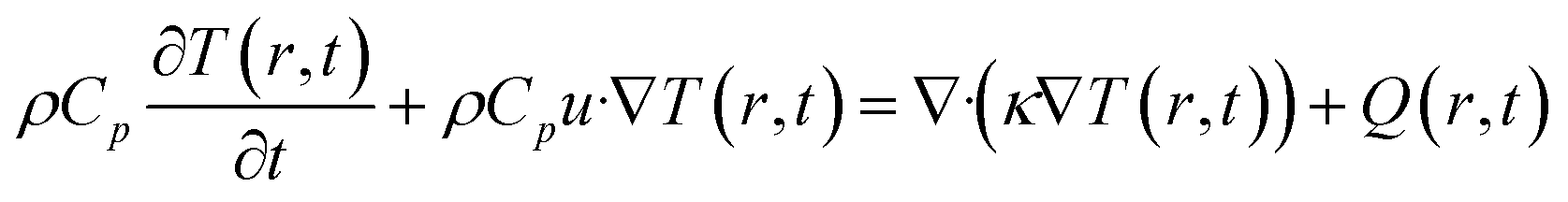
The numerical results obtained are based on a modelization of the MALDI process using rate equations, including the Fourier transform of heat transfer and, hence, the sublimation effects and the dependence on the radiation parameters (see ref. 19 for further details). We used three layers whose thicknesses vary as a function of the simulation parameters.Temperature calculation
For this calculation, we follow the same theoretical treatment discussed in ref. 19, in which a three-layer energy–matter balance model was used. The model is derived from the Fourier theorem, as given by eqn (1):
 | (1) |
If we include the effects of radiation and sublimation, and after some mathematical treatment, eqn (1) yields:
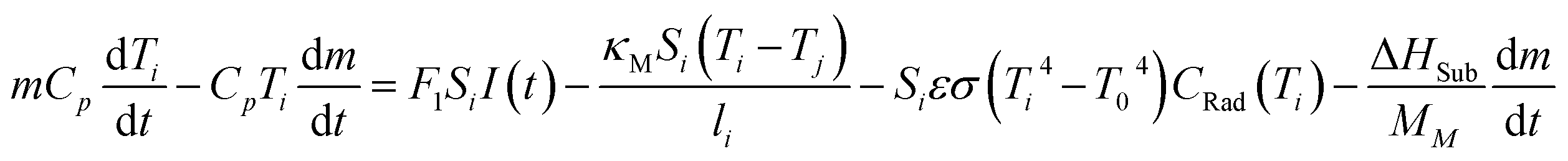 | (2) |
The area of the matrix irradiated by the laser can be considered by including a “coverage” fraction factor χM. This is included in factor F1 of eqn (2), and is equal to χM(1 − RM), where RM is the reflection coefficient. It is important to emphasize that the layer thickness, li, is calculated using the absorption coefficient αM,λ times a factor Δβ,19 as shown in eqn (3):
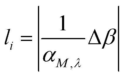 | (3) |
The idea behind the use of the factor Δβ is to prevent the temperature of the second layer reaching the sublimation temperature (TSub).
For the calculations,30 we applied the following stepwise procedure:
(1) A fluence is selected.
(2) An arbitrary value of Δβ is given.
(3) The calculation is carried out. Then:
(3.1) If T of 2 layer > TSub, then Δβ is increasing. Go to step 3.
(3.2) If T of 2 layer < TSub, then Δβ is decreasing. Go to step 3.
(3.3) If T of 2 layer = TSub of sublimation, then Δβ is the value sought and l is determined by eqn (3).
When T = TSub, the thicknesses of the three layers are assumed to be equal. Besides, it is considered that the thickness of the layers is >750 nm, so the metal substrate of the sample does not play an important role in the heat dissipation (from the matrix towards the metal).
The described approach was employed to calculate the rises in temperature suffered by the matrix layers and their variation as a function of time. When the laser irradiates the matrix, the crystalized molecules deposited on the metal substrate start to gain energy from the radiation, i.e., they are heated, leading to a swift phase transition when TSub is reached. It should be noted that this process occurs because the energy dissipation by the crystalline structure is not fast enough. Thus, while the laser is still active, molecules are transferred into the gas phase.
In fact, the transference of molecules from the solid to gas phase continues beyond the duration of the laser pulse until the excess energy is dissipated. Thus, the molecules existing in the gas phase become a supersaturated molecular ensemble, which enables an increase above TSub. This was confirmed by the simulations we carried out, where the surface temperature remained above the sublimation temperature for a long time after the laser pulse had ceased. This time can reach even the microsecond timescale for high laser fluence. The whole process in MALDI resembles the dynamics of supersonic beams, with the ejected molecules achieving velocities above the speed of sound by energy transfer from the laser radiation (see ref. 18 and 19 and ESI† of this work). Therefore, a thermodynamic adiabatic correction to pressure and density might be applicable.27
Another important aspect that must be considered is, that since the laser heating persists for a longer time than the pulse duration, the first portion of sublimated molecules, i.e., those molecules sublimated while the laser is still active, can acquire further energy by interacting in the gas phase with the radiation. This result is crucial, especially in UV-MALDI where laser radiation may favour the positive and negative ion yield via photonic effects. In other words, measurements carried out with no time-lag-focusing28 or short delay extraction time, in comparison to the laser lifetime, will differ from those with medium or long times.
Thermal conductivity κ calculation
Although the thermal conductivity is an intrinsic property of every material or compound, it varies as a function of temperature. Thus, in our simulations for considering the heat diffusion between the different layers, it is necessary to calculate the thermal conductivity κ and the layer thickness, li, for every step of the procedure. Typically, when the temperature rises, the conductivity increases up to a maximum. Once it has reached this maximum value, it decreases but at a much slower rate than when it rises.For this work, data of thermal conductivity κ for the matrices DHB, FA and CHCA were taken from the NIST database, although values over a large range of temperatures are scarce. Thus, aiming to reproduce the parameter behaviour, we adjusted the data sets numerically using power polynomials and Taylor series (cos(x) or sin(x)). Finally, a step function containing two sub-domains was achieved (see Fig. 1 in ESI†).
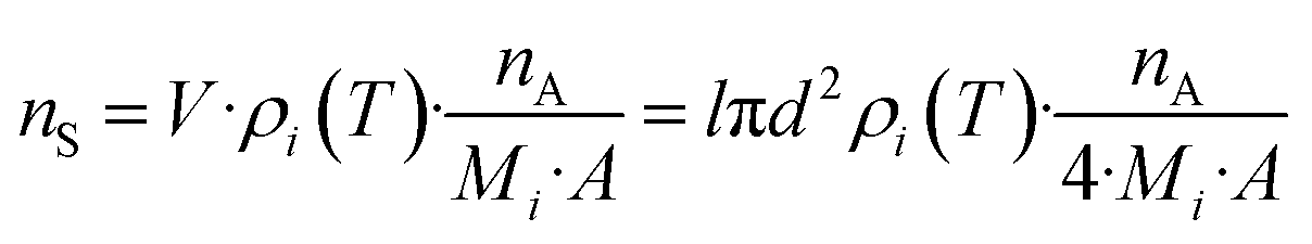
Calculation of number of molecules per square meter
One relevant parameter for obtaining a complete picture of MALDI dynamics is the number of molecules transferred into the gas phase per area (nS), which is basically related to the molecules existing in the sublimated layer. This parameter is easily derived from our calculation using eqn (4):
 | (4) |
 | (5) |
According to the previous discussion, eqn (5) accounts for density changes up to TSub. From this value on, a supersonic expansion correction factor is applied as well as a correction to the second layer, which emits heat in form of radiation.19
Fitting of trends, two-regime turning point and fluence threshold (FT)
Calculations were carried out between 100 mJ cm−2 and the lowest fluence value, for which the parameter Δβ could be adjusted so that the temperature of the second layer does not reach TSub. It is important to note that this fluence limit is not the fluence threshold, but the fluence for which the first layer becomes completely sublimated. This value corresponds to the layer threshold lT. Below this thickness, there is no value of Δβ for which the second layer achieves TSub. However, there is still a gradient of temperatures for the first layer and so for the rest.Meanwhile, if the temperature of the first layer passes TSub, partial sublimation occurs. Thus, the fluence threshold is calculated by fitting the data obtained from the simulation, assuming an extrapolation of the Δβ factor up to 3 Å. This value was chosen because it is meant to be the minimum van der Waals longitudinal interaction. It is important to notice that in the obtained data two trends are clearly distinguishable (see Fig. 6 and Discussion). This supports the hypothesis of two different regimes as a function of the laser fluence: i.e., desorption for low radiation fluences and ablation for high ones. The laser fluence at which there is a change from one regime to another is called the critical fluence FC.
The obtained data were adjusted to linear equations of the form:
| [Δβ, nS or l] = AΔβ + BΔβ·F | (6) |
Results and discussion
For the numerical simulations, we considered laser radiation at 355 nm wavelength and pulse duration of 4 ns (FWHM). This radiation is typically provided by frequency mixing of the fundamental output and its second-harmonic of an Nd![[thin space (1/6-em)]](https://www.rsc.org/images/entities/char_2009.gif) :YAG laser. The focus diameter was set to 100 μm, which seems reasonable for most experimental cases. A fluence range of 3 mJ cm−2 for DHB and CHCA, and 2.4 mJ cm−2 for FA, up to 100 mJ cm−2 was studied in the simulations. To account for the pulse durations, different power density ranges were used: 7.5 × 10⁹ W m−2 (DHB, CHCA) and 6 × 10⁹ W m−2 (FA) to 2.5 × 10¹¹ W m−2.
:YAG laser. The focus diameter was set to 100 μm, which seems reasonable for most experimental cases. A fluence range of 3 mJ cm−2 for DHB and CHCA, and 2.4 mJ cm−2 for FA, up to 100 mJ cm−2 was studied in the simulations. To account for the pulse durations, different power density ranges were used: 7.5 × 10⁹ W m−2 (DHB, CHCA) and 6 × 10⁹ W m−2 (FA) to 2.5 × 10¹¹ W m−2.
It must be mentioned, as we discussed above, that the deposition methods, i.e., the sample preparation, heavily influence the experimental results from MALDI. In simulations, this factor can be taken into consideration by adjusting the coverage fraction (χM). In our previous work,19 χM values of 0.95 and 0.85 were chosen. In this work, we considered χM = 1 in most situations, i.e., we assumed that the target is completely covered by, for example, sublimation or electrospray deposition methods. Nevertheless, for comparison purposes, we also analysed the situation of χDHB = 1 and χDHB = 0.85. This is shown in Fig. 4, where around a 15% difference in the Δβ factor was found.
In addition, we considered the following conditions:
(i) The laser beam irradiates the MALDI plate at normal incidence.
(ii) Expansion and evolution of the plume occur in the absence of an electrical field.
(iii) As a consequence of (ii), pulsed ion extraction is not in operation. The latter together with (i) and (ii) are typical conditions of an internal MALDI FT-ICR-MS set-up.
(v) Derived from (iv): no effects produced by laser-metal interaction are accounted for.
The parameters used in the calculation are summarized in Table 1.
| Parameter | DHB | FA | CHCA | Ref. |
|---|---|---|---|---|
| ri/m | 3.5 × 10⁻¹⁰ | 10.4 × 10⁻¹⁰ | 10.1 × 10⁻¹⁰ | Calc. by DFT |
| 1/αi /m @ 355 nm | 8.7 × 10⁻⁶ m | 1.25 × 10⁻⁷ m | 3.5 × 10⁻⁷ m | 23 and 29 |
| εi (W m−2 K−4) | 0.8 | 0.8 | 0.8 | Assumed |
| κi (W m−1 K−1) | f(T) | f(T) | f(T) | 31 and ESI |
| Cp,i (J mol−1) | f(T) | f(T) | f(T) | 23 and 29 |
| Mi (Kg mol−1) | 0.15412 | 0.194186 | 0.18917 | 31 |
| ΔHSub (J mol−1) | 1.17 × 10⁵ | 1.2 × 10⁵ | 1.071 105 | 31 |
| ρi (T = 298 K) (kg m−3) | 1.4 × 10³ | 1.123 103 | 1.4 103 | 31 |
| TSub/K | 450 | 445 | 460 | 31 |
Temperature variation and first derivative
The calculation of T variation as a function of time was carried out for three different matrices. Here we show a typical time-dependent T-profile for the DHB at a fluence of 4.1 mJ cm−2 (see Fig. 1). As it can be seen in Fig. 1, the temperature T of the second layer never reaches TSub. This is due to the adjustment of Δβ to a certain value.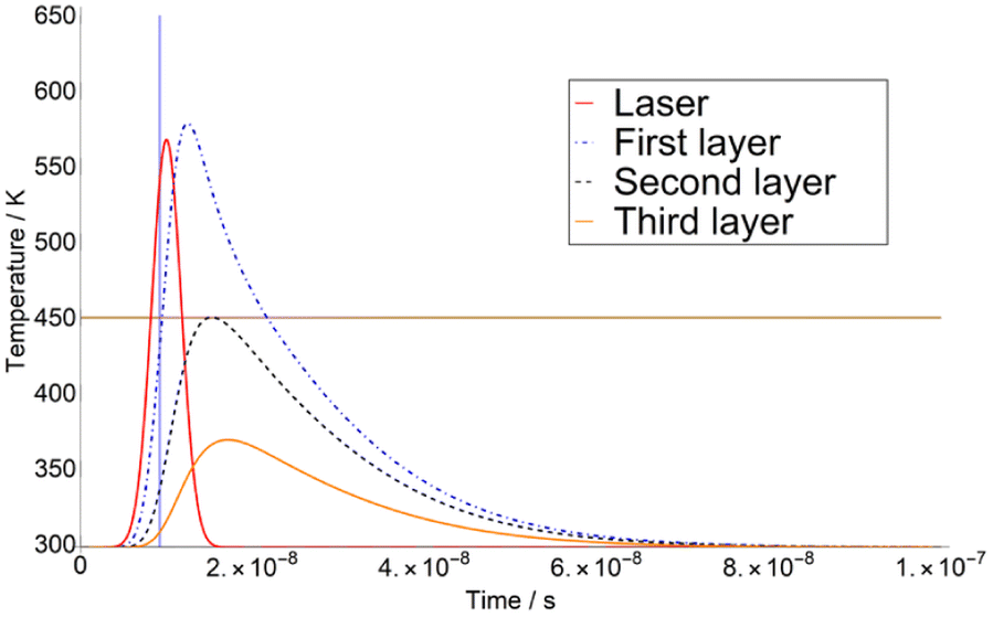 | ||
| Fig. 1 Temperature transients for DHB (χDHB = 1) according to the three-layer model for a fluence of 4.1 mJ cm−2. The horizontal brown line represents TS (450 K), and the blue vertical line the time when TSub is reached. | ||
The first derivatives of transients from Fig. 1 are plotted in Fig. 2. As it can be seen in Fig. 2, the temperature of the third layer T3 exhibits a maximum, i.e., the first derivative is zero, just when the laser radiation has almost ceased. This behaviour is similar at higher fluence, i.e., 7.5 mJ cm−2 in ESI,† for which the maximum of T3 takes place far later than the extinction of the laser pulse.
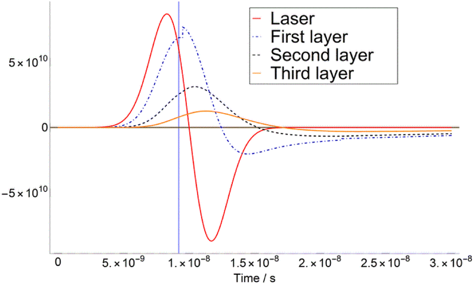 | ||
| Fig. 2 First derivatives of transients in Fig. 1 (4.1 mJ cm−2). The feature presented in the first layer is an effect of the adiabatic correction to the pressure and volume when T = TSub. (iv) It is assumed that after matrix deposition, 100% of the metal target is covered. | ||
According to these results, one can define a turning point at which the slope of Δβ as a function of the fluence F changes. The fluence at which this occurs is the so-called critical fluence FC and defines the transition between the two discussed regimes.15 Thus, if F < FC, the dominant regime is desorption, and there is a smooth transition from solid to gas. On the other hand, if F > FC, ablation is predominant, and a sudden overheating of the sample takes place. In our calculation, the value of FC was derived for the three chosen matrixes: DHB = 4.1 mJ cm−2, FA = 3.1 mJ cm−2 and CHCA = 7.1 mJ cm−2.
Δβ and fluence threshold, FT
Two series of data were chosen according to the fit of eqn (6). Values of the parameters BΔβ and Bl are collected in Table 2. Variation of Δβ as a function of the fluence for FA and CHCA matrices (DHB in ESI†) are compared in Fig. 3. It is interesting to note that the FA matrix shows a much faster rise than the CHCA one. In addition to this, both matrices exhibit different behaviour when the fluence falls below FC. Thus, the turning point for FA takes place at a lower fluence than for CHCA, therefore making FC higher for CHCA. Conversely the fluence threshold FT, extrapolated for Δβ = 3 Å, is lower for CHCA than for FA. Thus, the minimum fluence required to partially sublimate a matrix follows the trend: CHCA (1.73 mJ cm−2) < FA (1.89 mJ cm−2) < DHB (2.21 mJ cm−2).| Parameter | DHB132 | DHB0.8533 | FA134 | CHCA135 |
|---|---|---|---|---|
| a The subscripts 1 and 0.85 correspond to χM = 1 and 0.85 χM = 0.85, respectively. | ||||
| BΔβ for F > FC | 0.034 | 0.030 | 0.045 | 0.021 |
| BΔβ for F < FC | 0.017 | 0.015 | 0.021 | 0.0175 |
| FC (mJ cm−2) | 4.1 | 4.8 | 3.1 | 7.1 |
| FT (mJ cm−2) | 2.21 | 3.16 | 1.89 | 1.73 |
| lT1 Å−1 | 22.4 | 23.8 | 10.1 | |
| Bl for F < FC | 1.5 × 10⁻⁹ | 6.0 × 10⁻¹⁰ | ||
| Bl for F > FC | 7.2 × 10⁻¹⁰ | 5.0 × 10⁻¹⁰ | ||
| Unit cell data | DHB I | DHB II | ||
| a/Å | 4.911 | 5.545 | 4.5887 | 5.8182 |
| b/Å | 11.828 | 4.877 | 16.7619 | 9.5061 |
| c/Å | 11.058 | 23.3506 | 11.7853 | 15.461 |
| V/Å3 | 642.22 | 630.1 | 906.00 | 853.15 |
 /Å /Å |
9.26 | 11.26 | 11.04 | 10.3 |
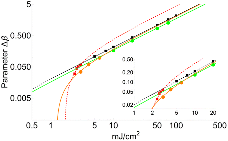 | ||
| Fig. 3 Trends of FA (squares) and CHCA (circles) for the two sets of data selected according to the best fitting criteria. The fluence at which the increase in Δβ varies as a function of fluence is different for both matrices. The threshold is higher for FA than CHCA (1.7 vs. 1.3 mJ cm−2). The inset shows an enlargement for fluences between 1 and 20 mJ cm−2. | ||
It is important to point out that the experimental measurements of FT and our calculated values are of the same order of magnitude. In fact, according to ref. 36 the FT value for DHB is close to 1.5 mJ cm−2, while our simulation yields 2.2 mJ cm−2. Also, this parameter FT for FA and CHCA has values of 4 and 2.5 mJ cm−2, respectively, according to the measurements carried out in ref. 23. These values are again slightly higher than those obtained in our calculations: 1.9 mJ cm−2 for FA and 1.7 mJ cm−2 for CHCA. We believe that a possible explanation for this disagreement resides in the ion transmission efficiencies of the ion optics and/or mass filters, which might have great difficulties detecting low amounts of neutrals.
Fig. 4 shows a comparison between two different coverage fractions, χDHB = 1 and χDHB = 0.85, in the inset, for a DHB matrix and its influence on the calculated parameters. The numerical results show that both FC and FT are higher for χDHB = 0.85 than for χDHB = 1. These interesting results agree with the observations carried out by Dreisewerd et al.22 In this work, the value of FT when first ions and/or neutrals are detected gets higher when the laser spot decreases, i.e., when the parameter χM gets smaller.
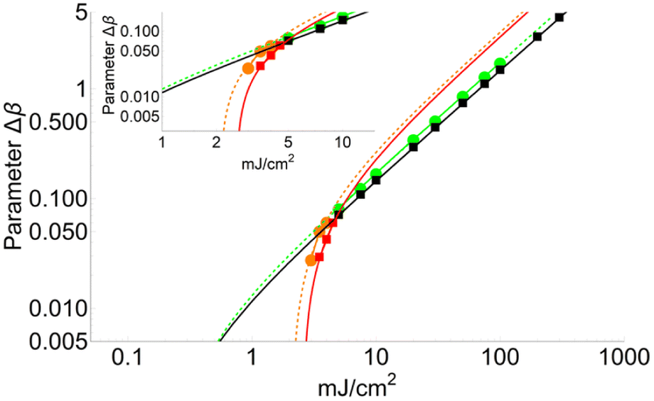 | ||
| Fig. 4 Variation of Δβ as a function of fluence for χDHB = 1 (circles) and χDHB = 0.85 (squares) for 100 μm laser-spot diameter. | ||
From Fig. 4, it is also possible to obtain a value for the fluence threshold and the critical fluence for the different coverage fractions considered: FT = 2.1 mJ cm−2 and FC = 4.1 mJ cm−2 for χDHB = 1, and FT = 2.6 mJ cm−2 and FC = 4.8 mJ cm−2 for χDHB = 0.85. Besides, Dresisewerd and coworkers in ref. 22 observed that the slope of the fitting decreased when the laser diameter was larger. In our simulations the slope diminishes from 0.034 to 0.030 (F < FC) and from 0.017 to 0.015 (F > FC). This means a reduction of 15%, which is observed both in FC and FT.
Sublimated thickness (l) and layer threshold (lT)
Fig. 5 shows the variation in thickness (l) as a function of fluence for FA and CHCA (DHB in ESI†). Since the variation of the layer desorbed per laser shot is proportional to Δβ, according to the results shown in Fig. 5, we can conclude that the layer depth affected by the laser and, therefore, totally transferred to the gas phase is higher for FA than CHCA. The slopes of the trends are quite similar: 7.2 × 10⁻¹⁰ and 5.0 × 10⁻¹⁰ for FA and CHCA, respectively, when F > FC, but quite different to lower fluences: 1.5.0 × 10−9 and 6.0 × 10⁻¹⁰ for FA and CHCA, respectively (F < FC). Also, the minimum layer desorbed for FA is 23.8 Angstroms (Å) while that for CHCA is 10.1 Å. This result is surprising if one compares it with those obtained from the structure of the crystalized matrix. In X-ray diffraction studies a 3D unit cell is identified for each substance and three different distances are given: a, b and c (see Table 2). Considering that in MALDI, crystals are randomly oriented, an average can be used as a reference. Thus, = 10.3 Å for CHCA and 11.04 Å for FA. Strikingly, the value for the latter almost corresponds to that obtained computationally but is almost twice the obtained experimental value.
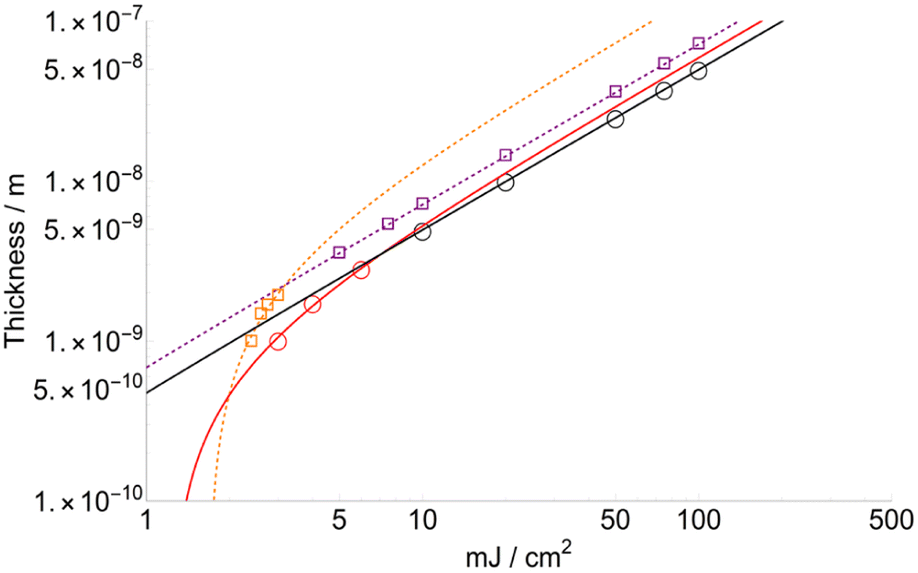 | ||
| Fig. 5 Thickness sublimated FA (squares) and CHCA (circles) for the two sets of data selected according to the best fitting criteria. | ||
Another interesting aspect is that calculations extended to DHB show a minimum thickness of 22.4 Å. This is also roughly double the average calculated from the unit cell:  = 11.3 Å. We believe that there is a relation between the minimum desorbed thicknesses and how molecules are located in the unit cell. Thus, CHCA molecules are oriented in co-planar layers differently than those from FA and DHB, whose molecular planes cross each other (ESI†). In other words, the interaction of the molecules via dispersive forces would basically be reflected by the macroscopic characteristics, such as the sublimation temperature, heat conductivity and heat capacity.
Number of molecules per square meter (nS)
The number of sublimated molecules per square meter can be calculated from eqn (4). Results for FA and CHCA are shown in Fig. 6 (DHB in ESI†). According to the results, the parameter nS increases much faster for low fluences (F < FC) than for high ones. This trend has been observed repeatedly for many years and recently confirmed by crossed molecular beam techniques.36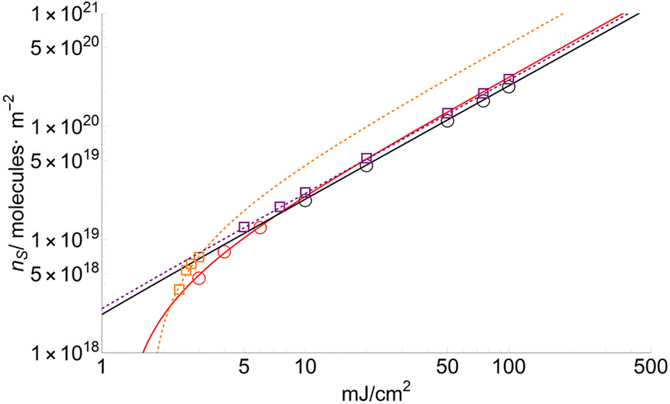 | ||
| Fig. 6 Number of molecules per square meter (ns) for FA (squares) and CHCA (circles) sublimated at different fluences. nFA and nCHCA are similar for fluences higher than 7 mJ cm−2. | ||
Fig. 7 displays the total number of molecules (N) surpassing the solid-to-gas phase barrier (ΔHSub) at low fluence for the three matrices.
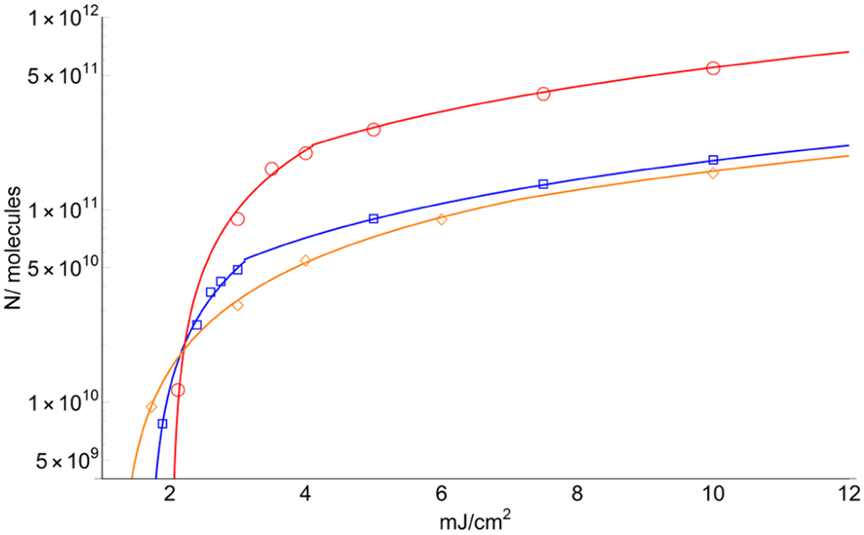 | ||
| Fig. 7 Number of total sublimated molecules (including those ionized) for DHB (circles), FA (square) and CHCA (rhomboid). Only the fit for data obtained for F > FC is shown. | ||
In the following, we compare the results obtained with the most recent, and in our experience the most accurate, data for the desorbed molecule. It is interesting to compare the increase in the calculated number of total molecules per shot per area (nS) with those from ref. 23, 37 and 38 It should be mentioned that C. K. Ni and co-workers23,37 employed cross-beam techniques for measurement, which is in our opinion the most powerful methodology so far, for the neutrals of the three matrices we have studied. In addition to these studies, we should note that there are not many articles where a quantitative analysis of the number of neutrals (N) and/or neutrals per area (nS) versus fluence can be found. For example, Niehaus et al.39 in 2018 published an excellent study showing qualitative trends that our work predicts. However, any attempt to compare this work with our data is not possible since the normalized photoacoustic signal from MALDI material ejection is given in arbitrary units. With an awareness of the scarcity of information existing in this sense, we refer the reader to the many good reviews published in the last two decades8,40–45 and references therein.
In Table 3, we record the data from ref. 23 and 37 calculated from the plots and divided by the laser spot: circular with a diameter of 200 μm diameter and 50 times 80 μm rectangular laser-spots, respectively. For this comparison, we have used the data plotted in Fig. 6 of our work for CHCA and FA and Fig. 3 of ESI,† where the thickness (l) of desorbed/ablated DHB is presented (with eqn (4) in which nS = (N/area). In general, we observed for all values close agreement of measurements to our predictions for all the matrices studied. In the case of DHB at lower fluence than the critical, an order of magnitude higher is predicted.
| Fluence mJ cm−2 | CHCA ref. 23 | CHCA this work | FA ref. 23 | FA this work | DHB ref. 37 | DHB this work |
|---|---|---|---|---|---|---|
| Neutrals shot/m2 | Neutrals shot/m2 (this work/ref. 23) | Neutrals shot/m2 | Neutrals shot/m2 (this work/ref. 23) | Neutrals shot/m2 | Neutrals shot/m2 (this work/ref. 37) | |
| a Predictions of this work divided by data from references are given in parentheses. | ||||||
| 2.5 | 1.5 × 10¹⁷ | 1.2 × 10¹⁹ (80.2) | ||||
| 5 | 2.0 × 10¹⁸ | 3.0 × 10¹⁹ (15.0) | ||||
| 10 | 9.5 × 10¹⁸ | 2.0 × 10¹⁹ (2.1) | 6.4 × 10¹⁸ | 2.2 × 10¹⁹ (3.5) | 5.0 × 10¹⁸ | 6.57 × 10¹⁹ (13.2) |
| 15 | 2.0 × 10¹⁹ | 1.1 × 10²⁰ (5.5) | ||||
| 20 | 6.4 × 10¹⁹ | 4.0 × 10¹⁹ (0.6) | 3.8 × 10¹⁹ | 5.0 × 10¹⁹ (1.3) | 3.7 × 10¹⁹ | 1.53 × 10²⁰ (4.1) |
| 25 | 5.0 × 10¹⁹ | 2.2 × 10²⁰ (4.0) | ||||
| 30 | 2.·1020 | 6.0 × 10¹⁹ (0.3) | 6.4 × 10¹⁹ | 7.0 × 10¹⁹ (1.1) | ||
In Table 4, we compare our predictions, obtained by interpolating our data with fitting equations, with those of ref. 38 for CHCA and DHB, where 1.5, 2, 3 and 4 times the threshold fluence were measured (0.30 and 0.87 μJ for CHCA and DHB, respectively, and an area of 0.0019 mm2 in both cases). According to the data, for CHCA the values predicted by our approach are around an order of magnitude higher than in ref. 38. However, for the DHB matrix this difference increases to two orders of magnitude.
| Fluence mJ cm−2 | CHCA ref 38 | CHCA this work | DHB ref 38 | DHB this work |
|---|---|---|---|---|
| Neutrals shot/m2 (1.5, 2, 3, 4 times threshold fluence) | Neutrals shot/m2 (this work/ref. 38) | Neutrals shot/m2 (1.5, 2, 3 times threshold fluence) | Neutrals shot/m2 (this work/ref. 38) | |
| a Predictions of this work divided by data from references are given in parenthesis. | ||||
| 24 | 5.0 × 10¹⁸ | 5.0 × 10¹⁹ (10.00) | ||
| 32 | 6.9 × 10¹⁸ | 7.0 × 10¹⁹ (10.2) | ||
| 47 | 1.7 × 10¹⁹ | 1.0 × 10²⁰ (6.0) | ||
| 63 | 2.3 × 10¹⁹ | 1.5 × 10²⁰ (6.6) | ||
| 69 | 1.6 × 10¹⁸ | 4.4 × 10²⁰ (275.0) | ||
| 92 | 2.5 × 10¹⁸ | 5.5 × 10²⁰ (220.7) | ||
| 137 | 4.5 × 10¹⁸ | 9.8 × 10²⁰ (221.0) | ||
It is interesting to pay close attention to these discrepancies with regard to the number of molecules (N). For the DHB matrix, we estimate an increase in neutrals of about 119 times for a fluence range between FT and 25 mJ cm−2. However, in ref. 23 this increase is nearly an order of magnitude higher (2500). For FA and CHCA and according again to ref. 37, the increase in neutrals for the same range of fluences is 200 for FA and 2000 for CHCA. However, we calculate increases of 59 and 41, respectively, which are significantly smaller. Thus, it seems clear that experiments show a faster increase in the number of neutrals as a function of fluence compared with theoretical results, e.g., one and two orders of magnitude for FA and CHCA-DHB, respectively. This observation is contrary to the (nS) results, for which the predictions show greater numbers.
We believe that this disagreement between theoretical and experimental results, and the aforementioned results corresponding to nS, has two different origins. On the one hand, the calculation of thermodynamical factors related to the processes of sublimation, radiation, and heat conduction, i.e., κ, Cp and f(T), could present some numerical inaccuracies. It is plausible that small inaccuracies could produce large discrepancies in the calculation of the relevant parameters in such highly correlated systems. On the other hand, and more importantly, a mechanical contribution should be introduced to consider the sudden loosening of material (chunks), i.e., a huge mass rate leaving the sample. In this situation, a compression effect defined by a force built rapidly. This force has the same magnitude but a different sign to that created by the material ejected from the surface. Including extra terms in the system of equations, where pressure (F → /area) is taken into account, would represent compensation for the temperature increase, giving rise to a more accurate description of the whole process.
Although the model presented in this work qualitatively describes the behaviour of thickness sublimation as a function of fluence as well as many other interesting features, e.g., the appearance of FT and FC, further work will be done to achieve better agreement between theoretical and experimental results.
Conclusions
In the work presented here, the three-layer energy–matter balance model was extended to the limit of the very low fluence threshold. Thus, two different regimes were encountered: desorption for fluences up to 4 or 7 mJ cm−2 (DHB or CHCA), and ablation from these fluences on. The two regimes are well identified by the variation in the sublimated number of molecules as a function of time. Furthermore, this approach applied to ns-UV-lasers based on rate equations describes a change in trend related to the transition in the dominant mechanism for ion production, i.e., related to the transition between adsorption and ablation, and establishes a turning-point fluence named the critical fluence FC. To the best of our knowledge, none of the previous attempts to simulate this behaviour in ns-MALDI was successful. We believe that our model can provide a phenomenological description of these processes because all the possible mechanisms competing between each other are included in our approach.Besides, the discussed model attempts to determine the limit of desorption, yielding values close to those measured by modern molecular crossed-beam techniques. The limit at which molecules (neutrals and/or ions) start to sublimate, known as the fluence threshold FT, is in our approach closer to the experimental values than the values theoretically predicted by the existing models. However, it fails in the description of the rapid increase in the total number of molecules as a function of fluence. Nevertheless, to the best of our knowledge, it provides the best qualitative results up to now.
For future work, it is necessary to devote more efforts to implementing mechanistic effects due to a force originating from the compression of the layer during sublimation. This will refine the model and will surely provide deeper insights. Furthermore, this thermo-mechanic model would explain the emission of chunks and spallation. These model refinements will be the subject of future publications.
Author contribution
E. Alonso: conceptualization, methodology, software, writing original draft. A. Peralta Conde: writing – review & editing, validation, visualization.Conflicts of interest
The authors declare no competing interests.Acknowledgements
We are grateful to Dr A. Lesarri for many helpful discussions and the revision of the manuscript.References
- M. Karas, D. Bachmann and F. Hillenkamp, Anal. Chem., 1985, 57, 2935 CrossRef CAS.
- M. Karas, D. Bachmann, U. Bahr and F. Hillenkamp, Int. J. Mass Spectrom. Ion Processes, 1987, 78, 53 CrossRef CAS.
- K. Tanaka, H. Waki, Y. Ido, S. Akita, Y. Yoshida and T. Yoshida, Rapid Commun. Mass Spectrom., 1988, 2, 151 CrossRef CAS.
- M. Karas and F. Hillenkamp, Anal. Chem., 1988, 60, 2299 CrossRef CAS PubMed.
- F. Hillenkamp, M. Karas, R. C. Beavis and B. T. Chait, Anal. Chem., 1991, 63, 1193A CrossRef CAS PubMed.
- M. B. O'Rourke, S. P. Djordjevic and M. P. Padula, Mass Spectr. Rev., 2018, 37, 217–228 CrossRef PubMed.
- R. Zenobi and R. Knochenmuss, Mass Spectrom. Rev., 1998, 17, 337–366 CrossRef CAS.
- R. Knochenmuss and R. Zenobi, Chem. Rev., 2003, 103(2), 441–452 CrossRef CAS PubMed.
- M. Karas and R. Kruger, Chem. Rev., 2003, 103(2), 427–439 CrossRef CAS PubMed.
- R. Knochenmuss, Analyst, 2006, 131(9), 966–986 RSC.
- K. Dreisewerd, Anal. Bioanal. Chem., 2014, 406(9–10), 2261–2278 CrossRef CAS PubMed.
- H. Awad, M. M. Kahmis and A. El-Aneed, Appl. Spectrosc. Rev., 2015, 50(2), 158–175 CrossRef CAS.
- L. V. Zhigilei and B. J. Garrison, Appl. Phys. Lett., 1999, 74, 1341 CrossRef CAS.
- Y. G. Yingling, L. V. Zhigilei, B. J. Garrison, A. Koubenakis, J. Labrakis and S. Georgiou, Appl. Phys. Lett., 2001, 78, 1631 CrossRef CAS.
- R. Knochenmuss, Electrospray and MALDI Mass Spectrometry, ed. R. B. Cole, Wiley, 2nd edn, 2010, ch. 5, section 5.2.1 Search PubMed.
- R. Knochenmuss, J. Am. Soc. Mass Spectrom., 2015, 26, 1645 CrossRef CAS PubMed.
- A. Vertes, R. Gijbels and F. Adams, Laser Ionization Mass Analysis, Chemical Analysis: A Series of Monographs on Analytical Chemistry and Its Applications, Wiley, 1993, vol. 164 Search PubMed.
- R. Knochenmuss, J. Mass Spectrom., 2002, 37, 867–877 CrossRef CAS PubMed.
- E. Alonso and R. Zenobi, Phys. Chem. Chem. Phys., 2016, 18, 19574 RSC.
- R. E. Johnson and B. U. R. Sundqvist, Int. J. Mass Spectrom. Ion Processes, 1994, 139, 25 CrossRef CAS.
- A. P. Quist, T. Huth-Fehre and B. U. R. Sundqvist, Rapid Commun. Mass Spectrom., 1994, 8, 149 CrossRef CAS.
- K. Dreisewerd, M. Schürenberg, M. Karas and F. Hillenkamp, Int. J. Mass Spectrom. Ion Processes, 1995, 141, 127 CrossRef CAS.
- I. C. Lu, K. Y. Chu, C. Y. Lin, S. Y. Wu, Y. A. Dyakov, J. L. Chen, A. Graz-Wale, Y. T. Lee and C. K. Ni, J. Am. Soc. Mass Spectrom., 2015, 26, 1242 CrossRef CAS PubMed.
- R. Knochenmuss, J. Am. Soc. Mass Spectrom., 2015, 26, 1645 CrossRef CAS PubMed.
- P. B. S. Kodali, L. V. Zhigilei and B. J. Garrison, Nucl. Instrum. Methods Phys. Res., Sect. B, 1999, 153, 167 CrossRef CAS.
- L. V. Zhigilei, P. B. S. Kodali and B. J. Garrison, J. Phys. Chem. B, 1997, 101, 2028 CrossRef CAS.
- G. Scoles, Atomic and Molecular Beam Methods, Oxford University Press, 1988, vol. 1 Search PubMed.
- W. C. Wiley and I. H. McLaren, Rev. Sci. Instrum., 1955, 26, 1150 CrossRef CAS.
- K. Y. Chu, S. Lee, M. T. Tsai, I. C. Lu, Y. A. Dyakov, Y. H. Lai, Y. T. Lee and C. K. Ni, J. Am. Soc. Mass Spectrom., 2014, 25, 310 CrossRef CAS PubMed.
- Wolfram Research, Inc, Mathematica, Version, 2022, 13, 2 Search PubMed.
- http://wtt-pro.nist.gov/wtt-pro/.
- D. E. Cohen, J. B. Benedict, B. Morlan, D. T. Chiu and B. Kahr, Cryst. Growth Des., 2007, 7, 492 CrossRef CAS.
- M. S. Adam, M. J. Gutmann, C. K. Leech, D. S. Middlemiss, A. Parkin, L. H. Thomas and C. C. Wilson, New J. Chem., 2010, 34, 85 RSC.
- S. P. Thomas, M. S. Pavan and T. N. Guru Row, Cryst. Growth Des., 2012, 12, 6083 CrossRef CAS.
- M. Karas, I. Fournier and M. Bolte, Acta Crystallogr., 2005, E61, o383–o384 Search PubMed.
- C. W. Liang, C. H. Lee, Y. J. Lin, Y. T. Lee and C. K. Ni, J. Phys. Chem. B, 2013, 117, 5058 CrossRef CAS PubMed.
- M.-T. Tsai, S. Lee, I. C. Lu, K. Y. Chu, C.-W. Liang, C. H. Lee, Y. T. Lee and C. K. Ni, Rapid Commun. Mass Spectrom., 2013, 27(9), 955–963 CrossRef CAS PubMed.
- Y. J. Bae, J. C. Choe, J. H. Moon and M. S. Kim, J. Am. Soc. Mass Spectrom., 2013, 24(11), 1807–1815 CrossRef CAS PubMed.
- M. Niehaus and J. Soltwisch, Sci. Rep., 2018, 8, 7755 CrossRef PubMed.
- K. Dreisewerd, Chem. Rev., 2003, 103(2), 395–426 CrossRef CAS PubMed.
- I.-C. Lu, C. Lee, Y.-T. Lee and C.-K. Ni, Annu. Rev. Anal. Chem., 2015, 8(1), 21–39 CrossRef CAS PubMed.
- Y. J. Bae and M. S. Kim, Annu. Rev. Anal. Chem., 2015, 8(1), 41–60 CrossRef CAS PubMed.
- R. Knochenmuss, Annu. Rev. Anal. Chem., 2016, 9(1), 365–385 CrossRef PubMed.
- Y.-H. Lai and Y.-S. Wang, Mass Spectrom., 2017, 6(3), S0072 CrossRef PubMed.
- C. D. Calvano, A. Monopoli, T. R. I. Cataldi and F. Palmisano, Anal. Bioanal. Chem., 2018, 410(17), 4015–4038 CrossRef CAS PubMed.
Footnote |
| † Electronic supplementary information (ESI) available. See DOI: https://doi.org/10.1039/d2ra06069h |
| This journal is © The Royal Society of Chemistry 2023 |