
 Open Access Article
 This Open Access Article is licensed under a Creative Commons Attribution-Non Commercial 3.0 Unported Licence
Fast and high-resolution mapping of van der Waals forces of 2D materials interfaces with bimodal AFM
Victor G.
Gisbert
 and
Ricardo
Garcia
*
and
Ricardo
Garcia
*
Instituto de Ciencia de Materiales de Madrid, CSIC, c/Sor Juana Ines de la Cruz 3, 28049 Madrid, Spain. E-mail: r.garcia@csic.es
First published on 20th November 2023
Abstract
High-spatial resolution mapping of van der Waals forces is relevant in several fields ranging from nanotechnology to colloidal science. The emergence of two-dimensional heterostructures assembled by van der Waals interactions has enhanced the interest of those measurements. Several AFM methods have been developed to measure the adhesion force between an AFM probe and the material of interest. However, a reliable and high-resolution method to measure the Hamaker constant remains elusive. We demonstrate that an atomic force microscope operated in a bimodal configuration enables fast, quantitative, and high-resolution mapping of the Hamaker constant of interfaces. The method is applied to map the Hamaker constant of monolayer, bilayer and multilayer MoS2 surfaces. Those interfaces are characterized with Hamaker constant and spatial resolutions of, respectively, 0.1 eV and 50 nm.
Introduction
Long-range van der Waals interactions are relevant in many scientific fields and topics, including colloidal science, atomic force microscopy (AFM) and molecular self-assembly. Several applications, for example those relying on two-dimensional materials, would benefit from a fast, high-spatial resolution and quantitative method to characterize the van der Waals interaction.Within the AFM community, the interest in van der Waals forces arises due to at least two factors. First, van der Waals forces are essential components of the interaction force acting on the AFM tip. Therefore, their precise knowledge and determination drew attention from the scientific community from the early years.1–5 The evolution of AFM methods and probes has kept the interest in van der Waals interactions alive. Second, the emergence of 2D materials and van der Waals heterostructures6–8 underlines the need to develop fast and high-spatial resolution methods to measure van der Waals interactions.
Several AFM-based methods have been developed to determine the Hamaker constant (H) of materials and interfaces.9–30 Among them are quasistatic methods based on recording force–distance curves. In those methods, the Hamaker constant is deduced from the adhesion force value measured in the tip's approach or in the jump into contact discontinuity.9–14 Those methods, albeit useful, have some limitations. First, they require the measurement of a large number of force–distance curves. Second, the adhesion force is the result of different interactions. It might not be always possible to separate the van der Waals force from the other interactions.15 An approach based on friction force microscopy was applied to determine the Hamaker constant of graphite and MoS2 surfaces.16 Dynamic AFM methods such as tapping mode AFM were also proposed to determine the Hamaker constant.5,17,18 There the Hamaker constant was deduced by fitting the AFM observables with theoretical equations. However, those approaches have had very few experimental implementations.
In this context, the development of multifrequency AFM methods, namely bimodal AFM, to determine van der Waals forces at the nanoscale represents a significant advance.19–27 Material property mapping in bimodal AFM might be acquired simultaneously with topography imaging.28–30 Therefore, multifrequency methods are inherently faster than quasistatic or tapping mode approaches. A bimodal AFM operated in the amplitude modulation configuration was applied to generate Hamaker constant maps.27 There, the Hamaker constant was determined by using numerical approximations. Those approximations slowed down the generation of the material property maps.
Here we introduce a bimodal AFM method which enables a fast, direct, quantitative and high-spatial resolution mapping of the Hamaker constant of van der Waals materials. We provide maps of monolayer, bilayer and multilayer flakes of MoS2 deposited on silicon dioxide and gold substrates with spatial and Hamaker constant resolutions, respectively, of 50 nm and 0.1 eV. The accuracy of the bimodal AFM method to determine the Hamaker constant is tested by performing numerical simulations and by developing a self-consistent test.
Theory of bimodal AFM for van der Waals forces
The bimodal AFM method is implemented with an amplitude modulation–frequency modulation (AM–FM) configuration (Fig. 1).31–33 The first mode is controlled by an amplitude modulation (AM) feedback. The AM feedback tracks the topography by keeping the amplitude of the first mode, A1, constant. The second mode is controlled by a frequency modulation (FM) feedback. The FM feedback keeps the phase shift and amplitude of the second mode at fixed values by modifying, respectively, the driving frequency Δf2 and the driving force F2. We noted that in bimodal AFM, the modes are driven and processed simultaneously.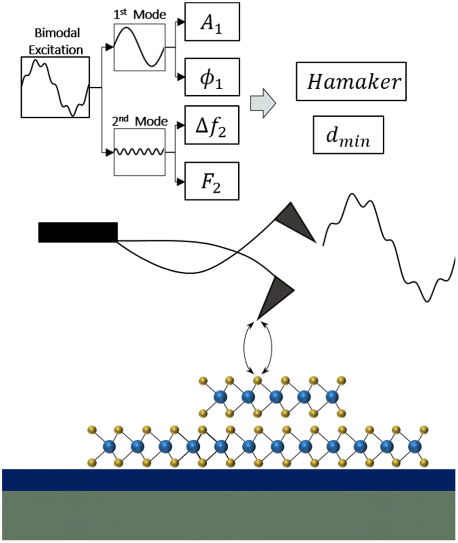 | ||
| Fig. 1 Scheme and observables of the bimodal AM–FM configuration implemented to map the Hamaker constant of 2D materials. The cantilever is simultaneously driven at the first and second resonances. An amplitude modulation feedback (AM) acts on the amplitude of the first mode, while a frequency modulation feedback (FM) controls the observables of the second mode. Analytical equations link the Hamaker constant of the material with the observables. | ||
The bimodal AM–FM configuration has been successfully applied to map nanomechanical properties in a variety of materials which include polymers,34–38 nanocomposites,39 self-assembled monolayers,40 Langmuir–Blodgett films,41 proteins,33,42 graphite43 and 2D materials.44 It has provided maps of the elastic modulus with angstrom-scale resolution.30 The bimodal AM–FM configuration has also been applied to measure long-range magnetic interactions.45 Therefore, it is a strong candidate for mapping van der Waals interactions.
To relate the bimodal AFM observables with the chemical composition of the substrate, the tip–sample interaction is modelled by using the van der Waals force for a sphere-plane geometry5,46
| F = −HR/6z2 | (1) |
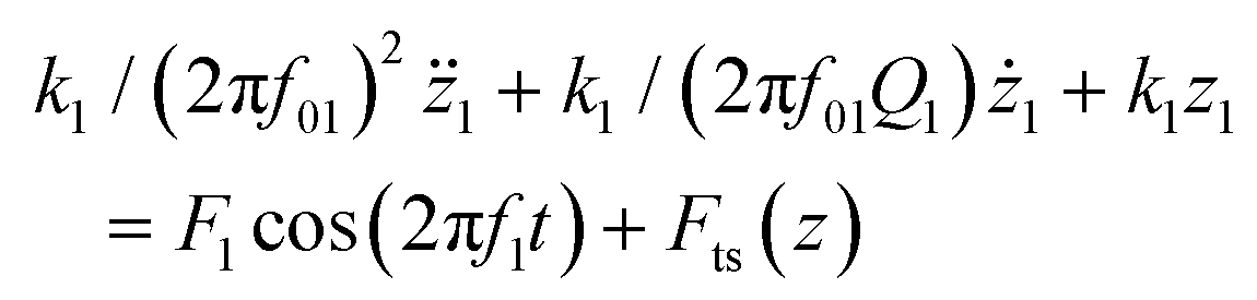
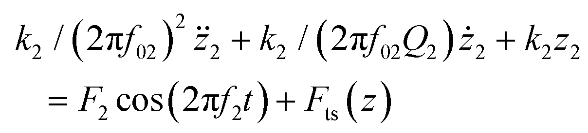
The theory and simulations were conducted with a two-eigenmode model of a rectangular cantilever beam described by the Euler–Bernoulli beam equation:46–48
 | (2) |
 | (3) |
The vertical displacement of the tip with respect to the sample surface is separated into two oscillatory components, one for each mode,
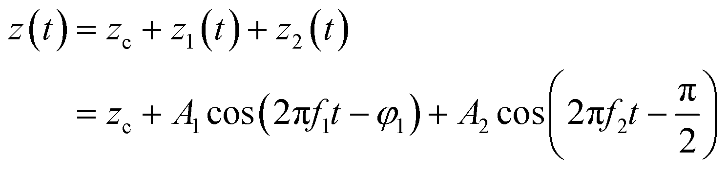 | (4) |
To link the observables with the interaction forces, we apply the virial theorem to the first and second modes5,47
 | (5) |
 | (6) |
For a long-range force of the form α/z2, the above equations yield22
| V1 = 2αA12/(zc2 − A12)3/2 | (7) |
| V2 = αA22(A12 + 2zc2)/(zc2 − A12)5/2 | (8) |
Analytical solutions to the virial equations might also be determined without an explicit knowledge of the interaction force46,47
| V1 = (k1A1A01/2Q1)cosφ1 | (9) |
| V2 = k2A22Δf2/f02 | (10) |
By combining eqn. (1), (7) and (8) we deduce an analytical relationship between the Hamaker constant and the observables
| α = HR/6 | (11) |
| H = 6A1V1/R((zc/A1)2 − 1)3/2 | (12) |
The average tip–sample distance is determined by
 | (13) |
| dmin = zc − A1 − A2 | (14) |
Materials and methods
Bimodal AFM
The bimodal AFM measurements are performed in a commercial AFM (Cypher S, Asylum Research-Oxford Instruments). The microscope is operated in the bimodal AM–FM configuration. The bimodal data are processed in real time with custom-made code. The topography and Hamaker constant maps are obtained in a single pass mode.We have used PPP-NCHAud (Nanosensors, Germany) cantilevers with f01 = 325 kHz, k1 = 40 N m−1, Q1 = 50, f02 = 2000 kHz, and k2 = 1600 N m−1. The tip radius was calibrated in each experiment by using the adhesion of the substrate as a reference.
The force constant of the first mode was calibrated by the multiple reference calibration method.49 To calibrate the spring constant of the second mode of the cantilever, we have used the power law relationship between the frequency and the stiffness:50k2 = k1(f2/f1)2.17. The bimodal AFM maps are obtained by avoiding the mechanical contact between the tip and the sample surface, which is usually called the attractive regime.46,51 To meet this requirement, ϕ1 must be above 90° and Δf2 ≤ 0.
Sample preparation
Flakes of molybdenum disulfide MoS2 (HQ Graphene, Netherlands) were mechanically exfoliated with adhesive tape and transferred onto a clean Si/SiO2 substrate using a polydimethylsiloxane (PDMS) stamp.8 The samples were sequentially ultrasonicated in acetone, isopropanol, and ultrapure water before deposition to remove organic contaminants. The ultrathin MoS2 flakes were afterwards heated at 300 °C for 1 hour. This step facilitated the removal of the moisture from the surface. Gold substrates were fabricated by e-beam evaporation. Flakes with thicknesses between 0.6 and 10 nm were selected by the color contrast obtained with an optical microscope.52 The bimodal AFM experiments were performed immediately after the samples were prepared.Results and discussion
Bimodal AM–FM of MoS2 deposited on SiO2
Fig. 2a shows, respectively, the topography of a multilayer MoS2 flake deposited on a silicon dioxide substrate. The flake height is about 8 nm. Fig. 2b shows an AFM phase image obtained with the first mode. The contrast in the phase shift signal is related to the energy transferred (dissipated) by the tip to the sample surface.17,46,53Fig. 2c shows an image obtained by plotting the frequency shift of the second mode on each position of the surface. The response of the frequency shift might be proportional to the gradient of the interaction force. Fig. 2d shows a map of the minimum distance to the sample surface. The minimum distance is determined by using eqn (14). The values of dmin are positive because the experiments are performed in the attractive regime.51,54 The values of dmin show spatial variations. Those variations reveal changes in the chemical composition of the sample. Fig. 2e shows the Hamaker constant map of the sample. The map shows two regions associated, respectively, with the SiO2 substrate and the multilayer flake. The cross-section (Fig. 2f) shows a value of the Hamaker constant for the multilayer (ML) flake of 0.8 eV while for the SiO2 substrate the value is about 0.4 eV. We note that within a given domain (ML or silicon dioxide) the Hamaker constant value hardly changes. This observation illustrates the reproducibility of the measurements.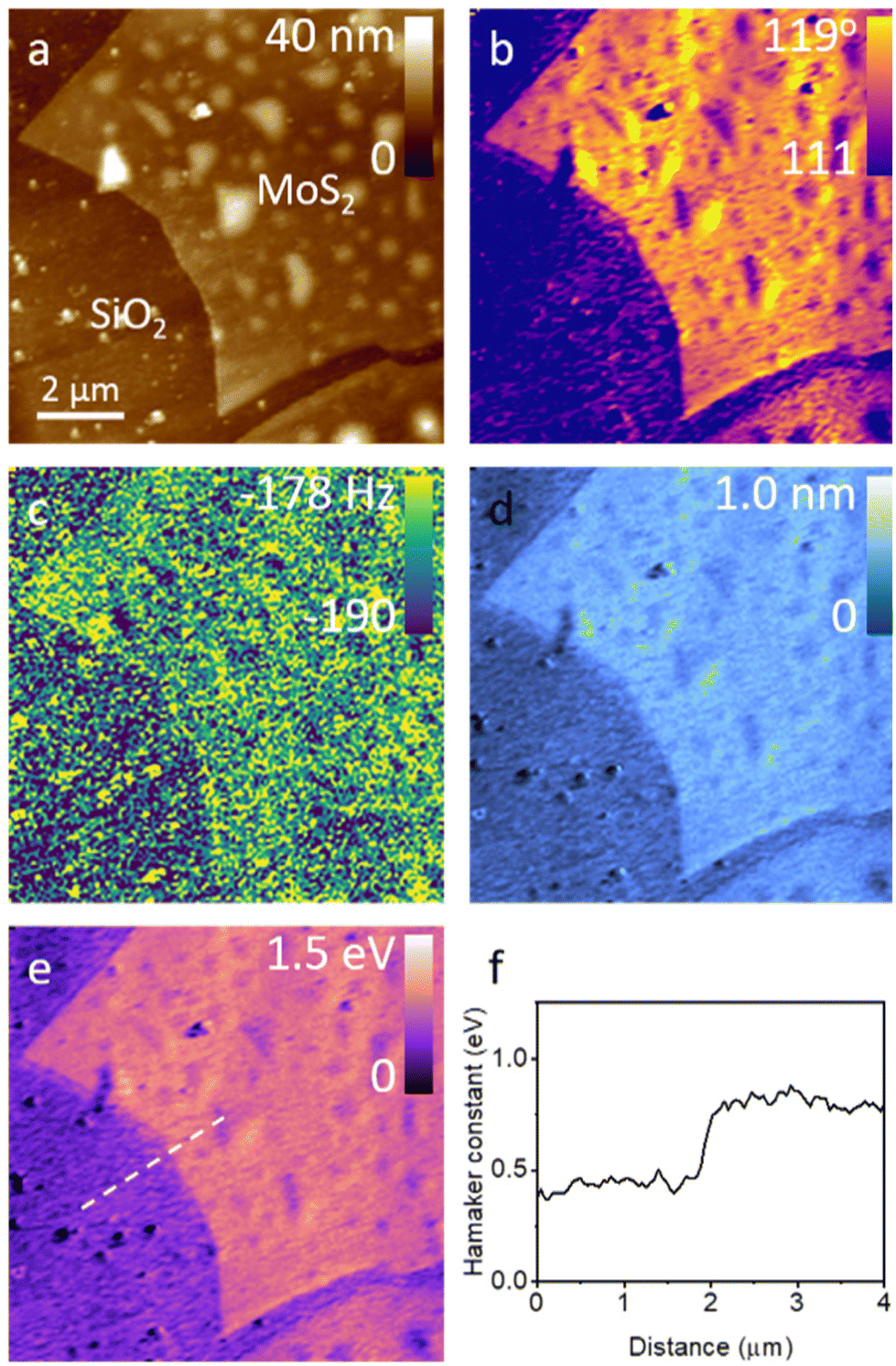 | ||
| Fig. 2 Bimodal AFM maps of MoS2 flakes deposited on SiO2. (a) Topography. (b) AFM phase image (first mode). (c) Frequency shift of the second mode. (d) Minimum distance between the tip and the sample. (e) Hamaker constant map. The map is obtained by processing (b–d) maps. (f) Cross-section along the dashed line marked in (e). It shows the variation of the Hamaker constant from the SiO2 surface to the MoS2 flake. Bimodal AFM parameters: A01 = 10 nm, A1 = 7.8 nm, A02 = 0.3 nm, f1 = 302 kHz, f2 = 1855 kHz, k1 = 41 N m−1, k2 = 1551 N m−1, and Q1 = 560. Scan line rate, 1 Hz; scan size, 11 μm; maps of 256 × 256 pixels. | ||
Bimodal AM–FM of MoS2 deposited on Au
Gold substrates were proposed to facilitate the exfoliation and deposition of single, double and triple monolayers of MoS2.55Fig. 3a shows a topography map of sections of the sample. By measuring the height with respect to the Au substrate we identify four regions: the Au substrate, and monolayer (1L), bilayer (2L) and trilayer (3L) domains of MoS2. In the AFM image, the height (thickness) of a monolayer is about 0.6 nm. Fig. 3b shows a map of the phase shift of the first mode. The map separates the Au substrate from the 1L, 2L and 3L regions. The 1L flake shows a contrast that lies between the Au and the 3L flake. The 2L and the 3L flakes show a similar contrast. Fig. 3c shows a map of the frequency shift of the second mode. Fig. 3d shows the map of dmin. The minimum distance between the tip and the sample in this experiment ranged between 0.2 nm (Au), 0.3 nm (1L) and 0.5 nm (2L/3L). This map reveals a clear contrast between the 2L/3L regions and the 1L and Au substrate. Fig. 3e shows the map of the Hamaker constant calculated from some of the previous maps. The map separates the Au from the 1L and the 2L/3L regions. We note that the map does not show differences between the 2L and 3L regions. From the Hamaker constant map, we infer a spatial resolution of about 50 nm. This value is obtained by considering the pixel size in the map (19.5 nm) and the consideration that 2–3 pixels are needed to show the transition from the Au substrate to the MoS2 flakes.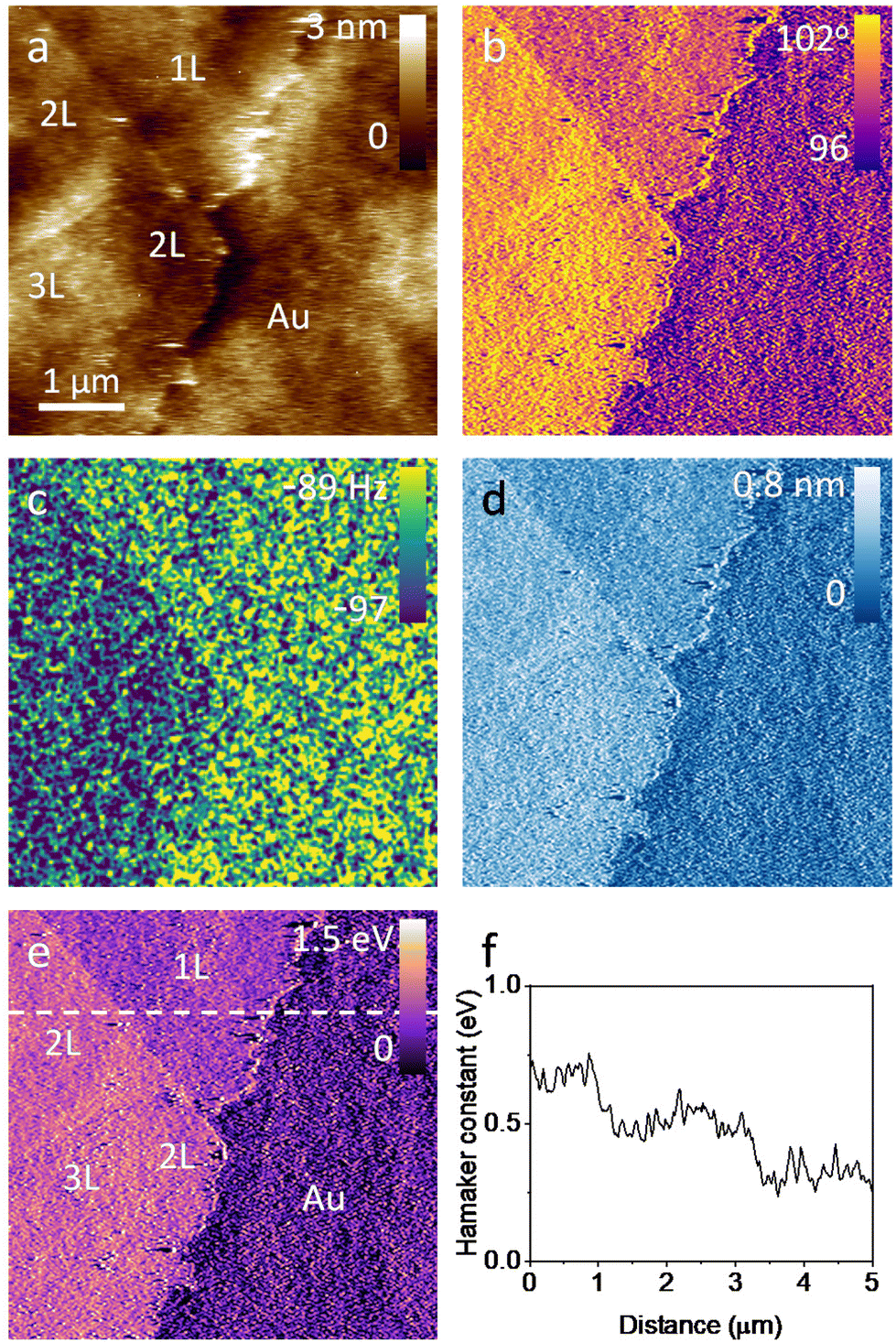 | ||
| Fig. 3 Bimodal AFM maps of MoS2 flakes deposited on Au. (a) Topography of a region of the interface with Au, monolayer (1L), bilayer (2L) and trilayer (3L) MoS2 domains. (b) AFM phase image (first mode). (c) Frequency shift map of the second mode. (d) Minimum distance between the tip and the sample. (e) Hamaker constant map of the interface. The map is obtained from the (b–d) maps. (f) Cross-section along the line marked in (e). The cross-section shows two transitions. Those transitions indicate the existence of three different surfaces. Bimodal AFM parameters: A01 = 13.5 nm, A1 = 12 nm, A02 = 0.4 nm, f1 = 284 kHz, f2 = 1805 kHz, k1 = 39 N m−1, k2 = 1558 N m−1, Q1 = 570. Scan line rate, 2 Hz; scan size, 5 μm; maps of 256 × 256 pixels. | ||
Fig. 3f quantifies the Hamaker constant values by showing a cross section of the Hamaker constant along the dashed line marked in Fig. 3e. The Hamaker constant varies from 0.75 eV (3L) to 0.5 eV (1L) to 0.3 eV (Au). The Hamaker constant values of a given region (3L, 2L, 1L or Au) do not depend on the spatial location within the region. The small fluctuations observed within a given region are attributed to the perturbations originating from the presence of the organic or water adsorbates that were not removed during the cleaning process.
Fig. 4 shows the histograms of the values of the Hamaker constant measured on Au, 1L and 2L MoS2 interfaces. The data show that the Hamaker constant of a bilayer (0.75 eV) is larger than the one of a single layer (0.5 eV) which is larger than the one of the Au substrate (0.25 eV). A similar trend was observed by Chiesa and co-workers on single, bilayer and multilayer graphene deposited on a Cu substrate.27
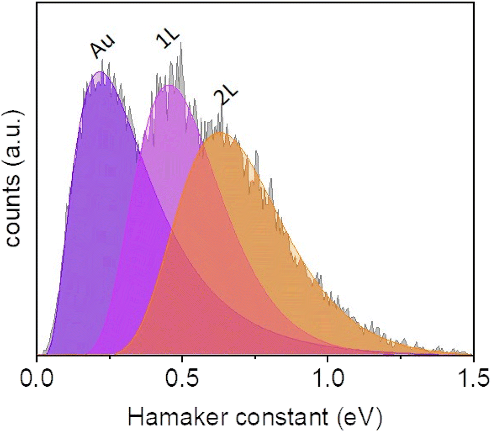 | ||
| Fig. 4 Histograms of the Hamaker constant values measured on Au, 1L and 2L MoS2 interfaces. The histograms are obtained from the map shown in Fig. 3e. The histograms provide the statistical support to the single cross-section shown in Fig. 3f. | ||
The above histograms provide a statistical support of the sensitivity and robustness of the bimodal AFM method to separate the van der Waals interactions arising from 1L and 2L MoS2 flakes. Those histograms are obtained from the map shown in Fig. 3e.
The differences observed between the Hamaker constant of the single and bilayers are attributed to the wetting transparency of the monolayers.56 The total force sensed by the tip on top of a monolayer is a combination of the van der Waals force of the monolayer and the one arising from the Au substrate. The double and triple monolayers show the same value for the Hamaker constant. That value is very similar to the one obtained on a multilayer MoS2 flake (Fig. 2f). This observation indicates that the influence of the Au substrate disappears if the MoS2 flake includes two or more layers.
Validation of bimodal AM–FM to characterize van der Waals forces
To validate the accuracy of the bimodal AFM method, we perform a comparison between experiments and numerical simulations. The experiment involves mapping of a region of a bulk MoS2 flake at different setpoint amplitudes, A1. For example, by reducing A1 we reduce dmin, which in turn increases the strength of the van der Waals forces. In parallel, we use a numerical simulation platform, dForce,57,58 to simulate the bimodal AM–FM observables under the experimental conditions.Fig. 5a shows a comparison of the values of the virial of the first mode obtained in the experiment with the values obtained by using dForce 2.057 as a function of the amplitude ratio A1/A01. The simulations are performed by using the Hamaker constant value for a multilayer MoS2 flake obtained in the bimodal AM–FM experiments (HMoS2 ≈ 0.85 eV). In the amplitude ratio range of 0.7–0.9, the virial V1 increases by reducing A1/A01. A plateau is reached at A1/A01 = 0.7. This behavior is characteristic of amplitude modulation AFM, where the maximum force is reached typically around 60–70% of the amplitude setpoint, and from then on it decreases.46,51 The numerical simulations (continuous line) reproduce the experimental trend and, more importantly, show good agreement with the numerical values. Fig. 5b shows the dependence of V2 on A1/A01. The virial of the second mode reproduces the behavior observed in the first mode. The experimental values of V2 are quantitatively predicted by the numerical simulations. The agreement obtained between experiment and simulations validates the bimodal AFM methodology to measure the Hamaker constant. Furthermore, we calculate the Hamaker constant of a MoS2 flake as a function of the amplitude ratio. Fig. 5c shows that in the A1/A01 range of 0.7–0.9 the value remains about 0.9 eV which is very close to the value used in the simulations (0.85 eV). This result might be considered a self-consistent validation test of the accuracy of the bimodal AFM to determine the Hamaker constant of any material, in particular, 2D materials.
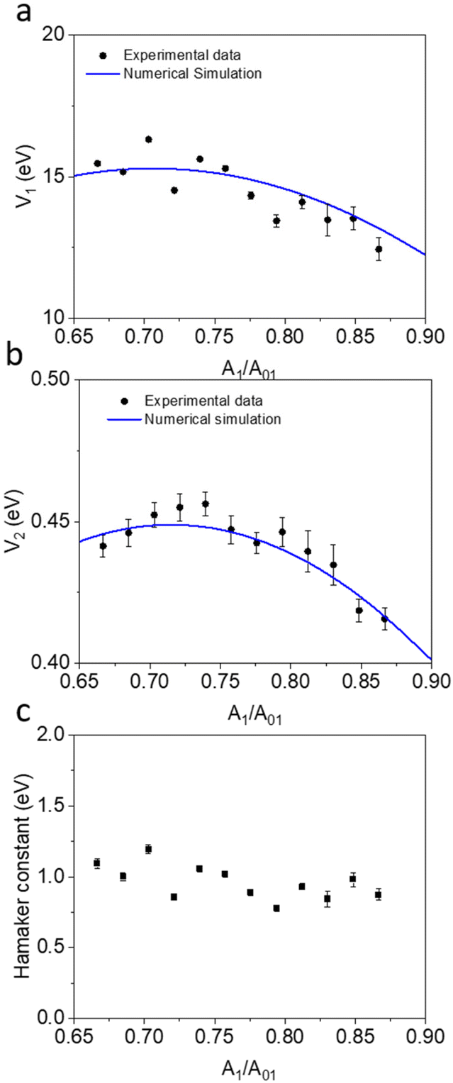 | ||
| Fig. 5 Validation of the bimodal AFM method to determine the Hamaker constant. (a) Virial of the first mode as a function of the amplitude ratio. The dots are the experimental values. The numerical simulation (continuous line) reproduces the experimental data. (b) Virial of the second mode as a function of the amplitude ratio. (c) Hamaker constant values obtained from the experimental data. Experimental and simulation parameters: A01 = 12.0 nm, A1 = 6.5–10.6 nm, A02 = 0.6 nm, f1 = 303 kHz, f2 = 1906 kHz, k1 = 41 N m−1, k2 = 2205 N m−1, and Q1 = 454. | ||
Conclusions
We developed a bimodal AFM method to map with nanoscale spatial resolution the Hamaker constant of heterogeneous 2D materials interfaces. The method is based on using a bimodal AM–FM configuration. The bimodal AFM method provides high-spatial resolution maps of the Hamaker constant of an interface formed by 1, 2 and 3 MoS2 monolayers deposited over a gold substrate. The map shows differences in the Hamaker constant among the Au, the 1L and 2L regions. The Hamaker constant values of the 2L, 3L and multilayers are very similar. This result indicates that the influence of the substrate disappears after the first two MoS2 layers.Key features of the method are its speed, quantitative accuracy and robustness. The method operates in a single pass by processing the data with analytical expressions. The analytical solutions make the mapping of van der Waals interactions fully compatible with the simultaneous imaging of the topography.
The robustness of the bimodal AFM method was tested by performing the measurements under operational conditions, namely amplitude ratios. We show that there is a range of values where the Hamaker constant values do not depend on the operational parameters.
The quantitative accuracy of the method was validated by comparing the data obtained in the experiments with the results obtained by using a numerical simulator.
In summary, we have expanded the capabilities of bimodal AFM by mapping the van der Waals interaction of complex heterogeneous 2D materials surfaces. We have demonstrated a spatial resolution of 50 nm and a Hamaker constant resolution of 0.1 eV.
Author contributions
VGG and RG conceived the project. VGG performed the experiments, developed the bimodal AFM code, and wrote the first draft of the manuscript. VGG and RG adapted the bimodal AFM theory for Hamaker coefficient mapping and analyzed the experimental data. RG wrote the final version of the manuscript.Conflicts of interest
There are no conflicts of interest to declare.Acknowledgements
We thank Francisco M. Espinosa for technical support with sample cleaning. Financial support from the Ministerio de Ciencia, Innovación y Universidades (PID2019-106801GB-I00 and PID2022-136851NB-I00) is acknowledged.References
- U. Hartman, Phys. Rev. B: Condens. Matter Mater. Phys., 1991, 43, 2404 CrossRef PubMed.
- N. Garcia and V. T. Binh, Phys. Rev. B: Condens. Matter Mater. Phys., 1992, 46, 7946 CrossRef PubMed.
- J. L. Hutter and J. Bechhoefer, Rev. Sci. Instrum., 1993, 64, 1868–1873 CrossRef CAS.
- C. Argento and R. H. French, J. Appl. Phys., 1996, 80, 6081 CrossRef CAS.
- A. San Paulo and R. Garcia, Phys. Rev. B: Condens. Matter Mater. Phys., 2001, 64, 193411 CrossRef.
- X. Liu and M. C. Hersam, Adv. Mater., 2018, 30, 1801586 CrossRef PubMed.
- R. Frisenda, E. Navarro-Moratalla, P. Gant, D. P. De Lara, P. Jarillo-Herrero, R. V. Gorbachev and A. Castellanos-Gomez, Chem. Soc. Rev., 2018, 47, 53–68 RSC.
- P. Ares and K. S. Novoselov, Nano Mater. Sci., 2022, 4, 3–9 CrossRef CAS.
- S. Das, P. A. Sreeram and A. K. Raychaudhuri, Nanotechnology, 2007, 18, 035501 CrossRef PubMed.
- S. G. Fronczak, C. A. Browne, E. C. Krenek, S. P. Beaudoin and D. S. Corti, J. Colloid Interface Sci., 2018, 517, 213–220 CrossRef CAS PubMed.
- B. Li, J. Yin, X. Liu, H. Wu, J. Li, X. Li and W. Guo, Nat. Nanotechnol., 2019, 14, 567–572 CrossRef CAS PubMed.
- Y. Li, S. Huang, C. Wei, D. Zhou, B. Li, C. Wu and V. N. Mochalin, ACS Appl. Mater. Interfaces, 2021, 13, 4682–4691 CrossRef CAS PubMed.
- B. Ku, F. van de Wetering, J. Bolten, B. Stel, M. A. van de Kerkhof and M. C. Lemme, Adv. Mater. Technol., 2023, 8, 2200411 CrossRef CAS.
- C. Cafolla, K. Voïtchovsky and A. F. Payam, Nanotechnology, 2023, 34, 505714 CrossRef PubMed.
- P. Lazar, S. Zhang, K. Safarova, Q. Li, J. P. Froning, J. Granatier, P. Hobza, R. Zboril, F. Besenbacher, M. Dong and M. Otyepka, ACS Nano, 2013, 7, 1646–1651 CrossRef CAS PubMed.
- B. A. Krajina, L. S. Kocherlakota and R. M. Overney, J. Chem. Phys., 2014, 141, 164707 CrossRef PubMed.
- R. Garcia, C. J. Gómez, N. F. Martinez, S. Patil, C. Dietz and R. Magerle, Phys. Rev. Lett., 2006, 97, 016103 CrossRef CAS PubMed.
- E. A. López-Guerra, S. Somnath, S. D. Solares, S. Jesse and G. Ferrini, Sci. Rep., 2019, 9, 12721 CrossRef PubMed.
- T. R. Rodrıguez and R. Garcia, Appl. Phys. Lett., 2004, 84, 449–451 CrossRef.
- C. Y. Lai, S. Santos and M. Chiesa, ACS Nano, 2016, 10, 6265–6272 CrossRef CAS PubMed.
- C. Y. Lai, S. Perri, S. Santos, R. Garcia and M. Chiesa, Nanoscale, 2016, 8, 9688–9694 RSC.
- R. Garcia, C. A. Amo and V. G. Gisbert, Spanish PatentES2781793A1, 07 September 2020 Search PubMed.
- C. Y. Lai, S. Santos, T. Moser, B. Alfakes, J. Y. Lu, T. Olukan, N. Rajput, T. Boström and M. Chiesa, Phys. Chem. Chem. Phys., 2020, 22, 4130–4137 RSC.
- S. R. Tamalampudi, S. Santos, C. Y. Lai, T. A. Olukan, J. Y. Lu, N. Rajput and M. Chiesa, Rev. Sci. Instrum., 2020, 91, 2 CrossRef PubMed.
- S. Santos, K. Gadelrab, L. Elsherbiny, X. Drexler, T. Olukan, J. Font, V. Barcons and M. Chiesa, J. Chem. Phys., 2023, 158, 204703 CrossRef CAS PubMed.
- S. Santos, K. Gadelrab, T. Olukan, J. Font, V. Barcons and M. Chiesa, Appl. Phys. Lett., 2023, 122, 7 CrossRef.
- Y. C. Chiou, T. A. Olukan, M. A. Almahri, H. Apostoleris, C. H. Chiu, C. Y. Lai, J. Y. Lu, S. Santos, I. Almansouri and M. Chiesa, Langmuir, 2018, 34, 12335–12343 CrossRef CAS PubMed.
- R. Garcia and E. T. Herruzo, Nat. Nanotechnol., 2012, 7, 217–226 CrossRef CAS PubMed.
- E. T. Herruzo, A. P. Perrino and R. Garcia, Nat. Commun., 2014, 5, 3126 CrossRef PubMed.
- S. Santos, C. Y. Lai, T. Olukan and M. Chiesa, Nanoscale, 2017, 9, 5038 RSC.
- C. A. Amo, A. P. Perrino, A. F. Payam and R. Garcia, ACS Nano, 2017, 11, 8650–8659 CrossRef CAS PubMed.
- M. Kocun, A. Labuda, W. Meinhold, I. Revenko and R. Proksch, ACS Nano, 2017, 11, 10097–10105 CrossRef CAS PubMed.
- S. Benaglia, V. G. Gisbert, A. P. Perrino, C. A. Amo and R. Garcia, Nat. Protocols, 2018, 13, 2890–2907 CAS.
- H. K. Nguyen, M. Ito and K. Nakajima, Jpn. J. Appl. Phys., 2016, 55, 08NB06 CrossRef.
- C. Dietz, Nanoscale, 2018, 10, 460 RSC.
- S. Benaglia, C. A. Amo and R. Garcia, Nanoscale, 2019, 11, 15289–15297 RSC.
- J. Hafner, S. Benaglia, F. Richheimer, M. Teuschel, F. J. Maier and A. Werner, et al. , Nat. Commun., 2021, 12, 152 CrossRef CAS PubMed.
- B. Rajabifar, A. Bajaj, R. Reifenberger, R. Proksch and A. Raman, Nanoscale, 2021, 13, 17428–17441 RSC.
- H. K. Nguyen, A. Shundo, X. Liang, S. Yamamoto, K. Tanaka and K. Nakajima, ACS Appl. Mater. Interfaces, 2022, 14(37), 42713–42722 CrossRef CAS PubMed.
- E. N. Athanasopoulou, N. Nianias, Q. K. Ong and F. Stellacci, Nanoscale, 2018, 10, 23027–23036 RSC.
- J. K. Wychowaniec, J. Moffat and A. Saiani, J. Mech. Behav. Biomed. Mater., 2021, 124, 104776 CrossRef CAS PubMed.
- M. Swierczewski, A. Chenneviere, L. T. Lee, P. Maroni and T. Bürgi, J. Colloid Interface Sci., 2023, 630, 28–36 CrossRef CAS PubMed.
- A. L. Eichhorn and C. Dietz, Adv. Mater. Interfaces, 2021, 8, 2101288 CrossRef CAS.
- Y. Li, C. Yu, Y. Gan, P. Jiang, J. Yu, Y. Ou, D. F. Zou, C. Huang, J. Wang, T. Jia, Q. Luo, X. F. Yu, H. Zhao, C. F. Gao and J. Li, npj Comput. Mater., 2018, 4, 49 CrossRef.
- V. G. Gisbert, C. Amo, M. Jafaar, A. Asenjo and R. Garcia, Nanoscale, 2021, 13, 2026–2033 RSC.
- R. Garcia, Amplitude modulation atomic force microscopy, John Wiley & Sons, 2011 Search PubMed.
- J. R. Lozano and R. Garcia, Phys. Rev. Lett., 2008, 100, 076102 CrossRef PubMed.
- S. D. Solares and G. Chawla, Meas. Sci. Technol., 2010, 21, 125502 CrossRef.
- J. E. Sader, R. Borgani, C. T. Gibson, D. B. Haviland, M. J. Higgins, J. I. Kilpatrick, J. Lu, P. Mulvaney, C. J. Shearer, A. D. Slattery, P.-A. Thorén, J. Tran, H. Zhang, H. Zhang and T. Zheng, Rev. Sci. Instrum., 2016, 87, 093711 CrossRef PubMed.
- A. Labuda, M. Kocuń, W. Meinhold, D. Walters and R. Proksch, Beilstein J. Nanotechnol., 2016, 7, 970–982 CrossRef CAS PubMed.
- R. Garcia and A. San Paulo, Phys. Rev. B: Condens. Matter Mater. Phys., 1999, 60, 4961 CrossRef CAS.
- H. Li, J. Wu, X. Huang, G. Lu, J. Yang, X. Lu, Q. Xiong and H. Zhang, ACS Nano, 2013, 7, 10344–10353 CrossRef CAS PubMed.
- S. Chiodini, J. Kerfoot, G. Venturi, S. Mignuzzi, E. M. Alexeev, B. T. Rosa, S. Tongay, T. Taniguchi, K. Watanabe, A. C. Ferrari and A. Ambrosio, ACS Nano, 2022, 16, 7589–7604 CrossRef CAS PubMed.
- A. San Paulo and R. Garcia, Biophys. J., 2000, 78, 1599–1605 CrossRef CAS PubMed.
- M. Velický, A. Rodriguez, M. Bouša, A. V. Krayev, M. Vondráček, J. Honolka, M. Ahmadi, G. E. Donnelly, F. Huang, H. D. Abruña, K. S. Novoselov and O. Frank, J. Phys. Chem. Lett., 2020, 11, 6112–6118 CrossRef PubMed.
- S. Tsoi, P. Dev, A. L. Friedman, R. Stine, J. T. Robinson, T. L. Reinecke and P. E. Sheehan, ACS Nano, 2014, 8, 12410–12417 CrossRef CAS PubMed.
- V. G. Gisbert and R. Garcia, Soft Matter, 2023, 19, 5857–5868 RSC.
- H. V. Guzman, P. D. Garcia and R. Garcia, Beilstein J. Nanotechnol., 2015, 6, 369–379 CrossRef CAS PubMed.
| This journal is © The Royal Society of Chemistry 2023 |