Solvent controlled 2D structures of bottom-up fabricated nanoparticle superlattices

Abstract

We demonstrate that oleyl phosphate ligand-stabilized iron oxide nanocubes as building blocks can be assembled into 2D supercrystalline mono- and multilayers on flat YSZ substrates within a few minutes using a simple spin-coating process. As a bottom-up process, the growth takes place in a layer-by-layer mode and therefore by tuning the spin-coating parameters, the exact number of deposited monolayers can be controlled. Furthermore, ex situ scanning electron and atomic force microscopy as well as X-ray reflectivity measurements give evidence that the choice of solvent allows the control of the lattice type of the final supercrystalline monolayers. This observation can be assigned to the different Hansen solubilities of the solvents used for the nanoparticle dispersion because it determines the size and morphology of the ligand shell surrounding the nanoparticle core. Here, by using toluene and chloroform as solvents, it can be controlled whether the resulting monolayers are ordered in a square or hexagonal supercrystalline lattice.

---

1 Introduction

The excellent behavior of ligand-stabilized nanoparticles (NPs) to arrange themselves into highly ordered structures during fairly simple evaporation procedures has fueled scientific interest over the last few decades.^1,2 These NP superstructures have already shown enormous potential for the fabrication of new devices and materials due to their extraordinary mechanical,^3–7 electrical,^8,9 and optical properties.¹⁰ Due to their abundance and non-toxicity, iron oxide NPs in particular have been investigated heavily during the last two decades for application in green catalysis,^11,12 medicine, and biotechnology.^13,14 In order to fully take advantage of the self-assembly process, however, two main obstacles have to be overcome: (1) controlling the self-assembly process to such an extent that a fully homogeneous material with few defects can be produced in a reliable way and (2) developing and improving fabrication pathways that can be scaled up to satisfy industrial demands.

For the self-assembly of truncated nanocubes, a variety of different crystal superstructures were reported ranging from face-centered cubic (FCC),¹⁵ rhombohedral (RH),¹⁶ and body-centered tetragonal (BCT),^17,18 to simple cubic (SC)¹⁷ structures. The shape and faceting of the NP core were found to be a major factor in determining the resulting superlattice structure. For cubic NPs, it was shown by both experimental investigations using controlled ligand removal^19–22 and atomistic simulations^23–26 that the supercrystal lattice structure directly depends on the degree of truncation of the particles as long as the ligand shell is not masking the faceting of the NP cores. For perfectly cubic NPs, face–face interactions dominate the interparticle forces and the SC structure is the thermodynamically most stable lattice.²⁷ With increasing truncation of the cubes, the face–face interactions become weaker, and the ligand–ligand interactions play an increasingly important role in determining the crystal structure. Therefore, an evolution in the morphology of NPs from perfectly cubic (1. state) to truncated (2. state) towards spherical (3. state) is accompanied by an evolution in the balance of interparticle forces from a domination of face–face interactions (1. state) to an intermediate state (2. state) towards a ligand–ligand interaction dominated lattice (3. state). With this changing balance between interparticle forces, different structures of the NP superlattices are formed ranging from SC (1. state) to RH and BCT (2. state) towards FCC (3. state).^18,27–29

To further understand the formation of superlattices, not only the NP core but also the ligand shell, as the second constituent part of the building blocks of the lattice, has to be taken into consideration. Consequently, the importance of the ligands around the NPs was recognized from the very beginning of NP self-assembly research by investigations on the effect of different ligand length to core radius ratios on the supercrystal formation.³⁰ For faceted NP cores, the shape and solvation of the ligand shell actually determine whether the core morphology influences the supercrystal formation. Many researchers argue that in a so-called “good” solvent, the ligand shell is well solvated and the ligands swell and spread out, which effectively suppresses the face–face interaction between the faceted NP cores.^17,31–34 To quantify the solubility of the ligands in a given solvent, the Hansen solubility parameter was shown to be a useful tool, even though no clear boundary values were established to determine what exactly constitutes a “good” or “bad” solvent.^17,32,35,36 Furthermore, the solvation of the ligand shell depends on the evolution of the evaporation process. As more and more solvent molecules evaporate, the solvation of the ligand shell and the ligand–solvent interactions naturally decrease. It has further been established by in situ SAXS experiments that during the evaporation process, NPs form an initial prenucleation superlattice in an excess of solvent and rearrange into a different lattice during the final drying stage to adjust for the changing thermodynamic balance of forces in the dry, solvent-poor state.^{29,32,37–41,47} The understanding of the solvation process of the ligand shell in an excess of solvent and its influence on the formation of the initial, prenucleation superlattice structure become especially important for fast preparation techniques like spin-coating, for which the self-assembly duration is relatively short, compared to the self-assembly of bulk materials by the evaporation of solvents over days and weeks.^3,4

Here we demonstrate that by using spin-coating, monolayer controlled nanoparticle films can be prepared. Depending on the solubility of the ligands in the solvent that was used, we were able to “freeze” the particles in square or hexagonal lattices in a controlled way. By analyzing which crystal structure is formed in different solvents, we found that the statement that a well-solvated ligand shell masks the underlying faceting of the NP core is not correct in general. Our results indicate that in a “good” solvent, the ligands are nearly completely spread out in an excess of solvent, which causes the ligand shell to mirror the faceting of the NP core, as can be seen by the superlattice that is formed by the particles. In a “bad” solvent, however, the building blocks are spherical and self-assemble into hexagonal superlattices. In addition to controlling and “freezing” the NP superlattice type, we were also able to reliably control the number of deposited NP layers and determine the NP coverage on the whole sample. Furthermore, we demonstrate that the nanoparticle layers form in a layer-by-layer fashion exhibiting structural motifs known from atomistic growth processes.

2 Results and discussion

We investigated the spin-coating process as a way to prepare 2D NP superlattices on flat yttria-stabilized zirconia (YSZ) substrates. The YSZ substrates are atomically smooth, as we demonstrated in our surface structure analysis.⁴² The building blocks of these superlattices were slightly truncated cubic iron oxide NPs with a ligand shell of oleyl phosphate ligands dispersed in either toluene or chloroform. For all experiments nanoparticles from the same preparation batch were used. The oxide core side length is 14.5 ± 0.88 nm, as determined by transmission electron microscopy (TEM), see Fig. S1 and S2.†

The solvents were chosen to have different Hansen solubilities, so that with respect to the oleyl phosphate ligands of the particles, one of them constitutes a “good” solvent and the other constitutes a “bad” solvent. The total Hansen solubility takes three different interactions between the respective molecules into account: dipolar interactions, hydrogen bonding interactions and dispersion interactions. The relative energy distance (RED) between the ligand and the given solvent in the Hansen space has proven useful to quantify the solubility of ligands as it directly quantifies the strength of the interaction between the ligand and the solvent molecules. For oleyl phosphate the RED values were determined to be 1.4 for toluene and 1.0 for chloroform.³⁵ After the deposition of the NP dispersion the samples were first rotated at a slower rotation speed of 250 rpm, before all remaining dispersion was spun off in a second, faster rotation step. During the 250 rpm step, the rotation is slow enough, so that the NP dispersion is spread out over the sample surface without evaporating immediately, allowing the self-assembly to take place. Furthermore, by controlling and varying the duration of the slow rotation step from 20 seconds up to 210 seconds, we were able to regulate the duration of the self-assembly process. Therefore, the amount of deposited supercrystalline NP layers on the surface was controlled and we were able to deposit from 1 up to 5 and more monolayers onto the substrate by changing the duration of the slow rotation step (Fig. S3†). Additionally, the NP dispersion was slightly diluted for the toluene samples compared to the chloroform sample.

First, we will discuss the results for both solvents in the monolayer regime. The two samples shown in Fig. 1 have a very comparable total coverage for both solvents with an average of 1.1–1.3 monolayers of deposited particles as further verified by XRR measurements (see Fig. 4). Due to the considerably higher evaporation rate of chloroform (see the ESI†) the slow rotation step for the chloroform sample was only 20 s (sample-square) compared to the 120 s of the toluene sample (sample-hexa). The impact of using different solvents can be seen in Fig. 1, which shows the scanning electron microscopy (SEM) images of two samples with similar NP coverage but with a distinctly different crystal structure, which is directly dependent on the solvent used. For the toluene sample (sample-hexa) the 2D monolayers show a hexagonal ordering, while for the chloroform sample (sample-square) the particles are ordered in a square lattice, as illustrated for both by the fast Fourier transformation (FFT) pattern (Fig. 1C and D). The self-assembly takes place in both cases in a nearly perfect layer-by-layer mode, in which the first layer is nearly completed before the nucleation of the second layer starts. For sample-square, prepared in chloroform, the coverage of the first layer is higher as compared to sample-hexa. A possible explanation for this observation could be the smaller domain size of the cubic domains allowing a better “tiling” of the substrate surface with in-plane randomly oriented domains. Alternatively, an incomplete wetting of the YSZ substrate by both solvents could give rise to the observed uncovered areas in the first layer.

Fig. 1 SEM images of the samples prepared with different solvents. (A) Toluene, called sample-hexa and (B) chloroform, called sample-square. (C and D) Corresponding close-up SEM images and fast Fourier transformation showing the hexagonal (C) and square (D) lattice types of the NP superlattices.

The crystallinity depends on the actual duration of the slow rotation step and hence on the duration of the self-assembly process. Estimations of crystal domain sizes based on the SEM images for the samples show an average domain consisting of 50–100 building blocks (equals a domain size of 70–140 nanometer) for the 120 s self-assembly of the toluene sample (sample-hexa), while the 20 s chloroform sample (sample-square) only shows domains made up of 10–20 building blocks (equals a domains size of around 45–75 nm). In addition, features known from atomic scale surfaces can be recognized for both types of structures: well-ordered step edges with defined in-plane orientation can be identified, as well as regular in-plane grain boundaries between domains.

In order to explain the resulting lattice structures, the differences between the used solvents have to be taken into consideration. Since the relative energy difference (RED) between the ligand and solvent molecules is about 40% larger for toluene than for chloroform, the ligands around the NPs are expected to interdigitate and bend around the NPs to a considerably larger extent in toluene than in chloroform in order to reduce solvent–ligand interactions. Therefore, it is expected that the used solvents directly affect the shape and size of the solvation shell around the particles. To further investigate the properties of the ligand shell, we analyzed the single crystal domains from the SEM images of different samples (see Fig. S3†) and measured the average area of a building block and the average nearest neighbor distance (NND) between the NP cores (see Table S1†). However, for the hexagonal samples the average measured area of a single building block is 223.2 ± 0.2 nm² and the NND is 15.2 ± 0.1 nm, and for the square lattice we measured an average area of 268.7 ± 11.5 nm² and a NND of 17.5 ± 0.3 nm. This trend is in-line with the expected behavior of the ligands in a “good” or “bad” solvent. In the “good” solvent chloroform, the ligands are more stretched out, effectively increasing the size of the superlattice building blocks because of the stronger solvent–ligand interaction. In the “bad” toluene solvent, the ligands may interdigitate because of the weaker interaction with the solvent and bend around the particles, leading to an effectively smaller building block.

When increasing the duration of the slow rotation step, the number of nanoparticle layers can be increased in a controlled way, see the SEM images in Fig. S3.† Using toluene as the solvent, the hexagonal arrangement persists also in the second layer after 180 s for the slow rotation step (Fig. S3B†). In a three-layer system, a transition to a cubic arrangement was observed between the second and third layers (Fig. S3C†). Using chloroform as the solvent, 3–5 layer-thick nanoparticle films can be produced (see Fig. S3D–F†). The cubic arrangement persists for all film thicknesses, demonstrating its higher stability. The evolution of monolayers with increasing duration of the slow rotation step indicates that the layers grow in a way that is comparable to the layer-by-layer growth mode known from atomic crystallization. A comparison of all the measured samples with different slow rotation step durations shows that the crystal domain size increases with the self-assembly duration for both solvents. Importantly, the defects formed in the first layer in contact with the YSZ substrate are not filled up during the formation of subsequent layers, indicating a higher particle–particle interaction, as compared to the particle–substrate interaction for both the used solvents.

More information about the 3D structure and stacking of the nanoparticle layers can be obtained by a closer inspection of the SEM images. The SEM images in Fig. 2 show the stacking of the second NP layer on top of the first NP layer for sample-hexa and for sample-square, respectively. For sample-hexa the hexagonal 2D ordering of the first layer continues in the second NP layer in such a way that the particles of the second layer sit on top of the valleys between the particles of the first layer, indicative of an FCC or HCP-like stacking. This is observed close to the step edge, whereas further away from the step edge the nanoparticle lattice is distorted or relaxed. This indicates that the lattice parameter of the first layer is different below the second layer as compared to areas, where it is not covered by the second layer. On the other hand, for the square 2D ordering of sample-square, the particles of the second monolayer sit directly on top of the particles of the first layer characteristic for a simple cubic (SC) stacking (Fig. 2B).

Fig. 2 Stacking of two NP layers. (A) Sample-hexa showing that the particles of the first layer sit between the particles of the second layer, as expected for an HCP stacking. Blue lines indicate the hexagonal lattice of the nanoparticles on the top, second layer terrace. (B) Sample-square for which the particles of the first and the second layer sit on top of each other. Particles of the second layer are highlighted for better visibility.

To further investigate the different stackings of the samples AFM height measurements were performed. An exemplary AFM image of sample-hexa in Fig. 3 clearly shows the distinct height difference between the substrate (black), the first NP monolayer (brown) and the second layer (light yellow). By averaging over a total of 3 different AFM images, the height difference between the first and the second NP layers was found to be 14.1 ± 0.3 nm (see Table S2†). This is roughly 0.5 nm less than the edge-length of the NP core, indicating that the particles of the second row have in fact sunken into the first NP layer, characteristic for a closed packing. For a hexagonal closed packing of hard spheres, one would, however, expect a layer distance of 0.8165 × nearest neighbor distance, resulting in 12.4 nm, which is smaller than the experimentally observed layer distance. This may indicate that interparticle interaction within one layer is stronger than the layer–layer interaction.

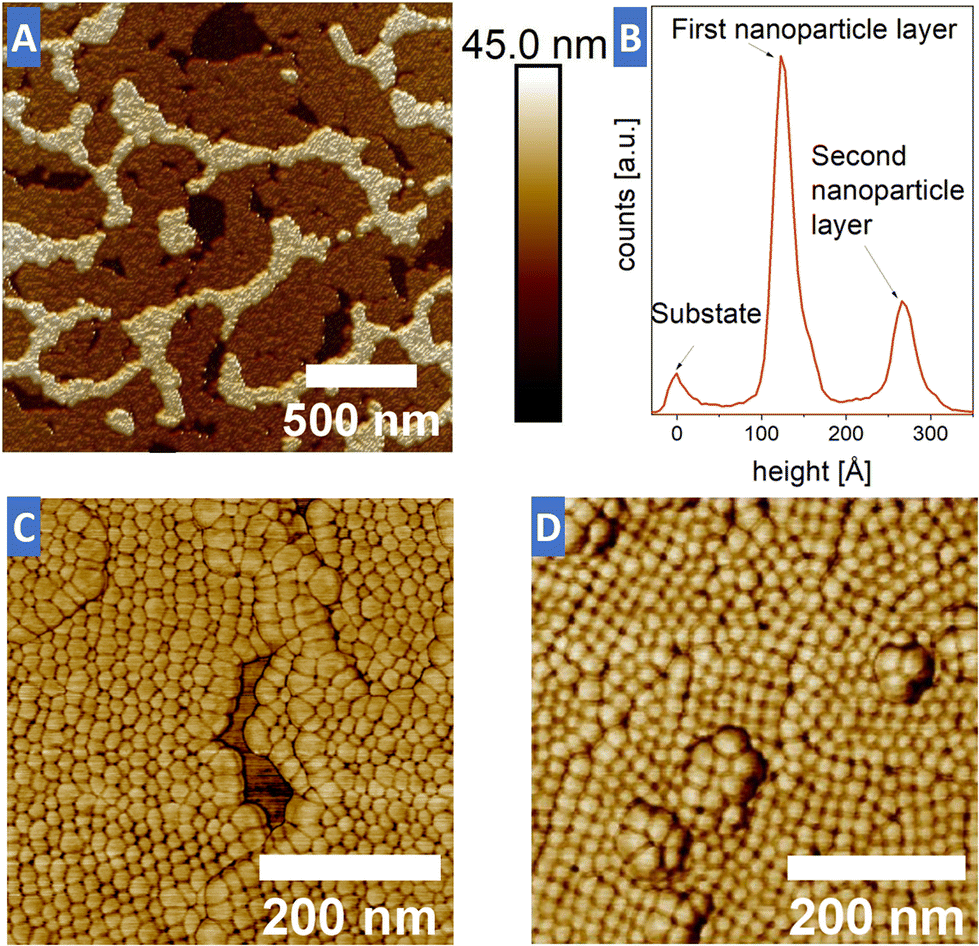Fig. 3 AFM images obtained from both types of samples. (A) AFM height scan image of sample-hexa in 3D. The image shows the coverage with the first monolayer of NPs (brown) with areas of a second NP layer on top (light yellow) and holes in the first layer which show the underlying substrate (black). (B) Average height distribution taken over the entire image in (A), showing three clear peaks associated with the substrate, the first level and the second NP level, respectively. (C and D) Nanoparticle resolved AFM phase image of sample-hexa and sample-square.

Furthermore, the height difference between the substrate and the first monolayer was measured to be just 12.5 ± 2.0 nm, which could be the result of residual ligands, extracted ligands and possibly impurities in the solvent being trapped in the holes of the first NP layer. Additional AFM phase images (Fig. 3C and D) show a very clear contrast resolving individual nanoparticles. The AFM images confirm the hexagonal and cubic arrangements obtained from the SEM images. The AFM results also show that the soft ligand shell interacts with the AFM tip. The apparent heterogeneity of particle sizes is the result of interactions between the AFM tip and the soft ligand shell, most pronounced at the edges of monolayers, since at that point the AFM tip has to travel the longest vertical distance and the ligands are less confined. Although this effect was almost negligible for sample-hexa, the AFM results for sample-cube indicate a much softer shell for the square ordered building blocks. This is especially evident for nanoparticle islands in the second layer, in which the nanoparticles appear larger and apparently two nanoparticles are imaged at the same time. This made it impossible to measure the individual layer thickness with comparable statistics to the ones performed for sample-hexa. The particle sizes are still homogeneous, as seen by SEM scans taken before and after the AFM scans, to exclude possible aging effects of the sample.

Additionally, we collected X-ray reflectivity (XRR) data to determine the electron density profile perpendicular to the surface. This allows us to obtain information on the stacking of the NPs and to correlate it with the AFM height measurements. In addition, the average total surface coverage can be determined with better statistics, as compared to the SEM images. Fig. 4 shows the XRR curves of sample-hexa (black) and sample-square (red) and the fits to the data. Both curves exhibit distinct, finite thickness oscillations, which are, however, more pronounced for sample-hexa. The inset in Fig. 4 shows the position of the minima of the two XRR curves. The distance between the minima of 0.49° (sample-hexa) and 0.51° (sample-square) in 2theta (diffraction angle) results in a corresponding effective layer thickness of around 15.4 nm in a simple one-layer model, which fits well to the NP diameter with their ligand shell (NP core diameter of 14.5 nm, see Fig. S1†).

Fig. 4 X-ray reflectivity curves of sample-hexa (black) and the corresponding fit (blue) as well as for sample-square (red) and the fit (green). Inset: position of the minima in the XRR curves for sample-hexa and sample-square.

The fits were performed with a 5-layer model, which was built from the bottom to the top as follows: 1. the YSZ substrate – 2. the bottom ligand layer – 3. the first NP layer – 4. the middle ligand layer – 5. the second NP layer and – 6. the top ligand layer. Fig. 5 shows the corresponding electron density profiles of the XRR curves in Fig. 4. The resulting thickness of the first NP layer fits very well to the edge length of the NP core of 14.5 nm (fitted values: sample-hexa = 14.5 nm and sample-square = 14.0 nm). The second NP layer, however, is too thin for sample-hexa (12.5 nm) and the middle ligand layer is thick and smeared out compared to sample-square (middle ligand layer thickness sample-hexa = 4.64 nm). This clearly indicates that for sample-hexa the particles in the second layer have slid between the particles of the first layer. For sample-square, the thickness of the second NP layer fits very well to the actual edge length of the particles (thickness of the second NP layer sample-square = 14.8 nm), which again clearly points toward a SC-like stacking. From the electron density profiles the NP layer distances can be determined. For sample-hexa we find 18.1 nm, which is significantly larger than the AFM value of 14.1 nm. This deviation can be explained by the fact that the thickness of the second nanoparticle layer in the profile is below the expected value of 14.5 nm for the magnetite nanoparticle core. Because of the interdigitation of the nanoparticle layers and the lower coverage of the second layer, the electron density profile has to be interpreted with care. For sample-square we determined a layer distance of 16.7 nm from the electron density profile, matching very well to the simple cubic stacking of the layers, leaving 2.2 nm space for the ligand layer. Overall, the XRR result fits well to the AFM height measurements, the small differences in the layer thicknesses are reasonably explained by the fact that with AFM only a small local spot of the sample is investigated, while the XRR curve contains contributions from a varying sample area. Although the distance between oscillation minima in the inset of Fig. 4 is very comparable, the curves show a distinct difference of 0.12° in the position of the first minima with respect to the total reflection edge. This shift can only be fitted with a different distance between the NP layers and the substrate, which resulted in a bottom layer thickness of 0.24 nm for sample-square and 2.37 nm for sample-hexa. Therefore, for sample-square there is possibly no, or only a very thin, ligand layer of completely bend ligands between the substrate and the NPs. Apparently, the more spread ligands in chloroform solution favor a face-to-face interaction of the flat nanoparticle facet and the substrate, leading to an expulsion of the ligands at the interface.

Fig. 5 Electron density profiles corresponding to the XRR curves in Fig. 4. (A) Sample-hexa and (B) sample-square. The upper part of the images shows the corresponding model of the NP cores and the ligand layers. For sample-hexa, the ligand layers are more smeared out as a result of the fact that the second row of particles sits inside the first row of particles. The electron density corresponds to the overall coverage of a given layer on the sample surface, therefore the different electron densities of the two nanoparticle layers is in line with the lower coverage of the second layer compared to the first layer.

Furthermore, the XRR results were used in combination with the SEM images to determine the exact coverage of the samples and the number of monolayers present. The electron density of each layer resulting from the fit of the XRR data corresponds to the average coverage of the given layer of the sample surface. Although the first nanoparticle layers cover the sample to a large extent, the coverage of the second layer on top of the first layer is much lower, as can be seen by the different electron densities of the two layers. By comparing the expected electron densities for an iron oxide layer with a coverage of 100% to the corresponding fit values of the samples, the coverage of each layer can be determined. The results fit very well to the SEM images and give a total coverage of 91.8% for sample-hexa with 36.9% of the first monolayer being covered by a second layer. Sample-square has a total coverage of 95.3% with 55.7% being covered by a second layer of NPs (see Table S3†). As discussed above, this incomplete coverage may result from an incomplete wetting of the YSZ surface by the solvents or from structural defects in the imperfectly growing layers.

Overall our measurements clearly show a solvent dependent formation of hexagonal lattices with FCC/HCP-like stacking for the toluene samples and square lattices with SC-like stacking for the chloroform samples. Since the solvents have a different Hansen solubility, the different lattice structures are most likely caused by a change in the ligand shell conformation around the particles, already indicated by the size and NND analyses of the SEM images. In order to explain how the solvation shell can influence the lattice structure of the NP superlattice, we need to consider both the thermodynamic and kinetic effects for the fast self-assembly process of spin-coating. From various model simulations and calculations, it is known that for slightly truncated cubes the SC crystal structure is the thermodynamically most stable one.^23–26

Furthermore, it was demonstrated that during the evaporation process NPs form an initial prenucleation superlattice in an excess of solvent before rearranging during the final drying stage to adjust for the changing thermodynamic balance of forces.^{29,32,38–41} Our ex situ measurements show distinct differences in the interparticle distances for the 2 solvents, which indicates a different arrangement of the ligand shell surrounding the particles. We argue that these differences are much more pronounced in the early stages of the self-assembly process as the number of solvent molecules that interact with the ligands is considerably higher in the prenucleation phase. Therefore, we propose that in the beginning of the self-assembly process, the diluted particles in the dispersion show a spherical shape in toluene due to the strongly bent and interdigitated ligands as a result of the high RED between the ligands and toluene. In this case, the dense ligand shells are effectively masking the faceting of the NP core. On the other hand, in chloroform with a 40% lower relative energy distance to oleyl phosphate compared to toluene, the ligands are supposed to spread out to increase the ligand–solvent interaction, so the ligand shell reflects the underlying cubic shape of the NP core to a larger extent. Another possible scenario which can also be considered is the strip-off of surface ligands by chloroform due to its high interaction with the ligands, leading to a predominant face-face interaction of the exposed facets. The impact of interaction between the dispersion agent and the ligand shell as one of the most important factors for the symmetry of the resulting superlattice has been observed recently and it was proposed as well that the ligand–solvent interaction influences the effective shape of the building blocks in solution.²⁸

As the evaporation proceeds the number of available solvent molecules decreases, so the particle concentration increases and the building blocks may start to interact with each other to eventually form a prenucleation lattice. Still in an excess of solvent, the ligand–solvent interactions dominate the interparticle forces and the particles in toluene form a hexagonal lattice and the particles in chloroform form a square lattice. As the drying process continues, less and less solvent molecules are present and the influence of the solvent–ligand interactions starts to decline. Since the thermodynamically most stable structure for the NP cores is the SC lattice caused by the dominance of face–face interactions between the cubes, we argue that the NP cores are driven to rearrange more and more toward the SC lattice structure as less and less solvent molecules are present. However, since the spin-coating process is fast, the solvent might dry too quickly for a complete rearrangement of the particles. Therefore, all chloroform samples (from 20 s to 120 s of self-assembly) may show SC ordering since the prenucleation lattice of the particles matches the most thermodynamically stable crystal structure in the dried state. For the hexagonally ordered building blocks in toluene, a full rearrangement from a hexagonal ordering to a SC lattice cannot be achieved during the short drying stage and the particles may be kinetically trapped in their prenucleation lattice. Looking in more detail at the toluene samples one can see a difference between very short (20 s–120 s) and slightly longer (210 s) self-assembly durations. For a very short self-assembly only hexagonal ordering was observed in the SEM images. For the slightly longer self-assembly duration (210 s, Fig. S3C†), only the first two NP monolayers show a mainly hexagonal ordering, while parts of the third layer have rearranged into a square lattice. Since the evolution of SEM images indicates a growth similar to the layer-by-layer like growth mode known from atomic crystallization, for the particles in the third monolayer the duration of the self-assembly is argued to have been sufficiently long for a rearrangement into a thermodynamically most stable crystal lattice.

3 Conclusions

Our results show that spin-coating is a suitable process to grow 2D supercrystalline lattices of cubic iron oxide nanoparticles with oleyl phosphate ligands onto flat YSZ substrates within a few minutes. Furthermore, by controlling the exact durations of the spin-coating steps we were able to effectively control the duration of the self-assembly process and thereby the number of deposited monolayers from a single monolayer up to more than five layers. A comparison of the resulting crystal lattices from different NP dispersions revealed that the 2D lattice type of the buildings blocks can be tuned by the used solvent: we obtained hexagonally ordered particle layers by using toluene and a square order of the particles by using chloroform as the solvent. Our analysis indicates that the different 2D lattice types and the stacking of the supercrystal structures may be explained by a solvent dependent ligand conformation. This is quantified by the difference in the Hansen solubility of the ligands in the solvent, which determines the size and morphology of the supercrystal building blocks during the self-assembly process. The spin-coating process discussed here opens up the possibility of layer-wise, controlled surface nanoparticle coating, allowing one to obtain nanoparticle functionalized surfaces for various applications. In addition, the prepared 2D layers can serve as templates for a more controlled growth of nanoparticle-based 3D bulk materials.

4 Experimental

4.1 Nanoparticle synthesis

All chemicals were used as received. The synthesis of the functionalized NP dispersion was performed according to ref. 43 followed by a post-synthesis ligand exchange as described in a previous publication,³⁵ yielding slightly truncated cubic iron oxide NPs with oleyl phosphate ligands with an average edge length of 14.5 ± 0.88 nm as determined by TEM measurements (see Fig. S1 and S2†). The NPs were dispersed in toluene and chloroform, with a respective particle concentration of 1.4 μM. The purification procedure³⁵ for the NP dispersion was repeated until the organic content could not be further decreased, in total nine times.

4.2 Spin-coating

Spin-coating experiments were performed by depositing a droplet of NP dispersion onto a flat and chemically inert YSZ single crystal substrate under an ambient atmosphere and at room temperature. YSZ substrates were cleaned thoroughly by the following steps: immersion in hydrochloric acid (37%) and ultrapure water (18.2 MΩ cm) and then by immersion twice in isopropanol followed by drying under a nitrogen stream. For all toluene samples, a 40 μL droplet of the undiluted NP dispersion (c = 1.4 μM) was placed on the substrate, and the NPs were deposited on the substrate in a time range of 20–210 s at 250 rpm. At the end, the excess of the dispersion was immediately removed by a subsequent interval at 1500 rpm for 60 s. The concentration had to be lowered for sample-square to reach a coverage of just around 1 monolayer with the quickly evaporating chloroform solvent. Therefore, 70 μL of 0.4 μM nanoparticle dispersion in chloroform were used while keeping the other spin coating parameters constant.

4.3 X-ray reflectivity measurements

All samples were measured at the laboratory X-ray source of the DESY Nanolab.⁴⁴ The setup used was a 6-circle diffractometer with a copper source generating a monochromatic X-ray beam with a wavelength of 1.5406 Å, which is a copper K_α X-ray emission line. The electron source spot size of the setup is 12 × 0.3 μm² (H × V) and the divergence of the beam is 0.4 mrad (V). All reflectivity curves were fitted with the software GenX,⁴⁵ which utilizes the well-known Parratt-formalism.⁴⁶

4.4 Scanning electron microscopy (SEM) and atomic force microscopy (AFM) measurements

SEM images of the samples in this work were taken using two different field emitter-based instruments, both with a lateral resolution of ∼1 nm, using a concentric back-scattered (CBS) detector. AFM topographic and phase images were obtained in tapping mode ex situ in air. Standard high resolution oxide-sharpened silicon cantilevers with a nominal spring constant of 40 N m⁻¹ and a resonant frequency of 300 kHz were used. The total sizes of the AFM images were chosen to be 2 μm × 2 μm and 500 nm × 500 nm, each with a resolution of 256 × 256 pixels and a scan rate of 0.5 Hz. The setpoint and gains were optimized for a least tip–sample interaction. For data analysis, the raw topographic images were corrected by a 2nd order flattening algorithm. For a description of the microscopes, see nanolab.desy.de.

Conflicts of interest

All authors declare no conflict of interest.

Acknowledgements

This project was funded by the Deutsche Forschungsgemeinschaft (DFG, German Research Foundation), project number 192346071, SFB 986 and by the Cluster of Excellence “Advanced Imaging of Matter” of the Deutsche Forschungsgemeinschaft (DFG) – EXC 2056 – project number 390715994. We acknowledge DESY (Hamburg, Germany), a member of the Helmholtz Association HGF, for the provision of experimental facilities.

References

1. E. V. Sturm and H. Cölfen, Crystals, 2017, 7(7), 207.
2. M. A. Boles, M. Engel and D. V. Talapin, Chem. Rev., 2016, 116, 11220–11289.
3. A. Dreyer, A. Feld, A. Kornowski, E. D. Yilmaz, H. Noei, A. Meyer, T. Krekeler, C. Jiao, A. Stierle, V. Abetz, H. Weller and G. A. Schneider, Nat. Mater., 2016, 15, 522–528.
4. B. Domènech, M. Kampferbeck, E. Larsson, T. Krekeler, B. Bor, D. Giuntini, M. Blankenburg, M. Ritter, M. Müller, T. Vossmeyer, H. Weller and G. A. Schneider, Sci. Rep., 2019, 9, 3435.
5. D. Giuntini, E. Torresani, K. T. Chan, M. Blankenburg, L. Saviot, B. Bor, B. Domènech, M. Shachar, M. Müller, E. A. Olevsky, J. E. Garay and G. A. Schneider, Nanoscale Adv., 2019, 1, 3139–3150.
6. P. Georgopanos, G. A. Schneider, A. Dreyer, U. A. Handge, V. Filiz, A. Feld, E. D. Yilmaz, T. Krekeler, M. Ritter, H. Weller and V. Abetz, Sci. Rep., 2017, 7, 7314.
7. A. Plunkett, M. Kampferbeck, B. Bor, U. Sazama, T. Krekeler, L. Bekaert, H. Noei, D. Giuntini, M. Fröba, A. Stierle, H. Weller, T. Vossmeyer, G. A. Schneider and B. Doménech, ACS Nano, 2022, 16, 11692–11707.
8. F. Fetzer, A. Maier, M. Hodas, O. Geladari, K. Braun, A. J. Meixner, F. Schreiber, A. Schnepf and M. Scheele, Nat. Commun., 2020, 11, 685.
9. Z. Nie, A. Petukhova and E. Kumacheva, Nat. Nanotechnol., 2010, 5, 15–25.
10. Y. Tong, E.-P. Yao, A. Manzi, E. Bladt, K. Wang, M. Döblinger, S. Bals, P. Müller-Buschbaum, A. S. Urban, L. Polavarapu and J. Feldmann, Adv. Mater., 2018, 30, 1801117.
11. E. Tajik, A. Naeimi and A. Amiri, Cellulose, 2018, 25, 915–923.
12. R. Irshad, K. Tahir, B. Li, A. Ahmad, A. R. Siddiqui and S. Nazir, J. Photochem. Photobiol., B, 2017, 170, 241–246.
13. C. A. Quinto, P. Mohindra, S. Tong and G. Bao, Nanoscale, 2015, 7, 12728–12736.
14. A. K. Gupta and M. Gupta, Biomaterials, 2005, 26, 3995–4021.
15. J. Brunner, I. A. Baburin, S. Sturm, K. Kvashnina, A. Rossberg, T. Pietsch, S. Andreev, E. Sturm and H. Cölfen, Adv. Mater. Interfaces, 2017, 4, 1600431.
16. J. J. Choi, K. Bian, W. J. Baumgardner, D.-M. Smilgies and T. Hanrath, Nano Lett., 2012, 12, 4791–4798.
17. Z. Quan, H. Xu, C. Wang, X. Wen, Y. Wang, J. Zhu, R. Li, C. J. Sheehan, Z. Wang, D.-M. Smilgies, Z. Luo and J. Fang, J. Am. Chem. Soc., 2014, 136, 1352–1359.
18. E. Wetterskog, A. Klapper, S. Disch, E. Josten, R. P. Hermann, U. Rücker, T. Brückel, L. Bergström and G. Salazar-Alvarez, Nanoscale, 2016, 8, 15571–15580.
19. J. C. da Silva, M. A. Smeaton, T. A. Dunbar, Y. Xu, D. M. Balazs, L. F. Kourkoutis and T. Hanrath, Nano Lett., 2020, 20, 5267–5274.
20. K. Whitham and T. Hanrath, J. Phys. Chem. Lett., 2017, 8, 2623–2628.
21. K. Whitham, D.-M. Smilgies and T. Hanrath, Chem. Mater., 2018, 30, 54–63.
22. Y. Wang, X. Peng, A. Abelson, P. Xiao, C. Qian, L. Yu, C. Ophus, P. Ercius, L.-W. Wang, M. Law and H. Zheng, Sci. Adv., 2019, 5, eaaw5623.
23. A. P. Gantapara, J. de Graaf, R. van Roij and M. Dijkstra, Phys. Rev. Lett., 2013, 111, 015501.
24. P. F. Damasceno, M. Engel and S. C. Glotzer, Science, 2012, 337, 453–457.
25. V. Thapar, T. Hanrath and F. A. Escobedo, Soft Matter, 2015, 11, 1481–1491.
26. D. Wan, C. X. Du, G. van Anders and S. C. Glotzer, J. Phys. Chem. B, 2019, 123, 9038–9043.
27. S. Disch, E. Wetterskog, R. P. Hermann, G. Salazar-Alvarez, P. Busch, T. Brückel, L. Bergström and S. Kamali, Nano Lett., 2011, 11, 1651–1656.
28. J. Schlotheuber, B. Maier, S. L. J. Thomä, F. Kirner, I. A. Baburin, D. Lapkin, R. Rosenberg, S. Sturm, D. Assalauova, J. Carnis, Y. Y. Kim, Z. Ren, F. Westermeier, S. Theiss, H. Borrmann, S. Polarz, A. Eychmüller, A. Lubk, I. A. Vartanyants, H. Cölfen, M. Zobel and E. V. Sturm, Chem. Mater., 2021, 33(23), 9119–9130.
29. X. Huang, J. Zhu, B. Ge, K. Deng, X. Wu, T. Xiao, T. Jiang, Z. Quan, Y. C. Cao and Z. Wang, J. Am. Chem. Soc., 2019, 141, 3198–3206.
30. B. A. Korgel and D. Fitzmaurice, Phys. Rev. B: Condens. Matter Mater. Phys., 1999, 59, 14191–14201.
31. Y. Zhang, F. Lu, D. van der Lelie and O. Gang, Phys. Rev. Lett., 2011, 107, 135701.
32. B. Lee, K. Littrell, Y. Sha and E. V. Shevchenko, J. Am. Chem. Soc., 2019, 141, 16651–16662.
33. K. Bian, J. J. Choi, A. Kaushik, P. Clancy, D.-M. Smilgies and T. Hanrath, ACS Nano, 2011, 5, 2815–2823.
34. S. W. Winslow, J. W. Swan and W. A. Tisdale, J. Am. Chem. Soc., 2020, 142, 9675–9685.
35. B. Domènech, A. Plunkett, M. Kampferbeck, M. Blankenburg, B. Bor, D. Giuntini, T. Krekeler, M. Wagstaffe, H. Noei, A. Stierle, M. Ritter, M. Müller, T. Vossmeyer, H. Weller and G. A. Schneider, Langmuir, 2019, 35, 13893–13903.
36. N. Goubet, J. Richardi, P.-A. Albouy and M.-P. Pileni, Adv. Funct. Mater., 2011, 21, 2693–2704.
37. F. Schulz, I. Lokteva, W. J. Parak and F. Lehmkühler, Part. Part. Syst. Charact., 2021, 38, 2100087.
38. I. Lokteva, M. Koof, M. Walther, G. Grübel and F. Lehmkühler, Small, 2019, 15, e1900438.
39. E. Josten, E. Wetterskog, A. Glavic, P. Boesecke, A. Feoktystov, E. Brauweiler-Reuters, U. Rücker, G. Salazar-Alvarez, T. Brückel and L. Bergström, Sci. Rep., 2017, 7, 2802.
40. J. J. Geuchies, C. van Overbeek, W. H. Evers, B. Goris, A. de Backer, A. P. Gantapara, F. T. Rabouw, J. Hilhorst, J. L. Peters, O. Konovalov, A. V. Petukhov, M. Dijkstra, L. D. A. Siebbeles, S. van Aert, S. Bals and D. Vanmaekelbergh, Nat. Mater., 2016, 15, 1248–1254.
41. M. Agthe, T. S. Plivelic, A. Labrador, L. Bergström and G. Salazar-Alvarez, Nano Lett., 2016, 16, 6838–6843.
42. V. Vonk, N. Khorshidi, A. Stierle and H. Dosch, Surf. Sci., 2013, 612, 69–76.
43. A. Feld, A. Weimer, A. Kornowski, N. Winckelmans, J.-P. Merkl, H. Kloust, R. Zierold, C. Schmidtke, T. Schotten, M. Riedner, S. Bals and H. Weller, ACS Nano, 2019, 13, 152–162.
44. A. Stierle, H. Noei, T. F. Keller, V. Vonk and R. Röhlsberger, J. Large-Scale Res. Facil., 2016, 2, A76.
45. M. Björck and G. Andersson, J. Appl. Crystallogr., 2007, 40, 1174–1178.
46. L. G. Parratt, Phys. Rev., 1954, 95, 359–369.
47. D. Monego, T. Kister, N. Kirkwood, D. Doblas, P. Mulvaney, T. Kraus and A. Widmer-Cooper, ACS Nano, 2020, 14, 5278–5287.

---

Footnote

† Electronic supplementary information (ESI) available. See DOI: https://doi.org/10.1039/d2nr03043h

---