Percolation of co-continuous domains in tapered copolymer networks
Received
1st August 2022
, Accepted 6th October 2022
First published on 7th October 2022
Abstract
Inhomogeneous polymer networks with bicontinuous morphologies have shown the potential to incorporate typically incompatible material properties into a single sample, and often the desired properties depend on co-continuity of the domains. Tapered copolymers have been shown to be useful for facilitating the formation of bicontinuous morphologies, though most applications are in linear diblock copolymers. We use coarse-grained molecular dynamics simulations to study inhomogeneous co-networks formed by tapered copolymers with different strand lengths, fractions of the minority domain and gradient lengths. Cluster and fractal analyses are performed to quantify the sizes of the clusters formed by the minority domain and to characterize the threshold for domain percolation. We find that the gradient length can be tuned to widen the composition window where bicontinuous percolating structures are found, and we show that the diffusion of tracer molecules selective for one phase is enhanced as the gradient length increases. Our results show how engineering the chemistry of the constituent polymers in a crosslinked material can allow tuning the material properties.
Design, System, Application
Polymer networks, including elastomers and hydrogels, find applications in a wide array of systems ranging from biomimetic materials and drug delivery vehicles to membranes and wearable devices. In many applications of crosslinked networks, the network system needs to provide seemingly disparate properties. For example, networks used as the electrolyte in lithium-ion batteries must allow for rapid Li ion transport while being mechanically robust to suppress dendrite growth. Having co-continuous domains that one facilitates transport and the other provides mechanical robustness is essential for this function, and as a result, there is a need to widen the range of compositions where one can obtain co-continuous domains. In this work, we use molecular simulations to show how creating networks from tapered copolymers significantly widens the composition window where one observes co-continuous networks. The transport properties of small molecules that only move through one of the domains can be greatly improved by engineering the copolymer strands. We believe our work will be useful for future experimental studies and for designing network systems requiring percolating co-continuous domains.
|
1 Introduction
Polymer networks, formed by the crosslinking of polymer strands and junctions, are an important class of soft matter.1–4 Over the past few decades, the development of synthetic chemistry and nanotechnology has led to the emergence of many novel classes of polymer networks with exceptional properties, such as covalent adaptable networks (CANs)5 and double networks (DN).6,7 Among them, inhomogeneous polymer networks composed of two components with bicontinuous morphologies have shown the potential to incorporate potentially disparate constituent properties. For example, Walker et al. have shown that co-networks formed by phase-separated poly(ethylene glycol) (PEG) and polystyrene (PS) are great candidates for solid-state electrolytes as the bicontinuous morphology allows the networks to achieve high storage modulus inherited from the PS phase as well as high ion conductivity inherited from the PEG phase.8
Polymeric materials with bicontinuous morphologies have drawn particular attention over the past few decades due to their promising applications in the field of polymer electrolytes and membranes.8–15 In diblock copolymer systems, the gyroid phase is thought to be promising for applications, but unfortunately this phase only forms in a narrow composition range.16,17 Co-networks, in contrast, can exhibit disordered bicontinuous morphologies over a broader range of volume fractions, as the addition of crosslinking junctions restrains the formation of ordered structures.8,18–22 Besides crosslinking the polymer blends, researchers have also developed other strategies to access bicontinuous morphologies, such as using multiblock copolymers23–26 and interfacially modified block copolymers.27–31 Roy et al. have shown that the ability of accessing the bicontinuous double gyroid phase can be improved by adding a gradient section (taper) between pure A and B blocks in AB diblock copolymers experimentally.27 Brown et al. and Seo et al. have used self-consistent field theory and molecular dynamics simulations to prove that adding tapers will further increase the miscibility between polymer blocks and make it easier to form the bicontinuous morphologies.29,31 The length of the gradient sections can also be tuned to control the domain spacing and phase behaviors.29,31 Therefore, one potential strategy for developing co-networks that are bicontinuous over a wide range of compositions could be to employ tapered copolymers.
In this work, we study tapered copolymer networks with different strand lengths (N), gradient section lengths (G) and fractions of the minority domain (fA) using coarse-grained molecular dynamics simulations. Cluster and fractal analyses are performed to quantify the sizes of the clusters formed by the minority domain. We verify that the co-continuous domains could be used for transport of small molecules by analyzing the mean square displacements calculated for tracer particles placed in the networks. Our results show that tapered copolymers are an effective strategy for widening the composition window where networks have co-continuous percolating domains.
2 Simulation methods
We conduct a hybrid of Monte Carlo simulations and coarse-grained molecular dynamics simulations to generate and equilibrate end-linked tapered copolymer networks. A reactive Monte Carlo method is used to construct the initial polymer network configurations from bifunctional polymer strands and tetrafunctional crosslinking junctions, and molecular dynamics (MD) simulations are then conducted to equilibrate the network systems. We describe the details of each step below.
2.1 Initial network generation
A reactive Monte Carlo method with irreversible reactions is used to generate the polymer network configurations, and our approach is intended to mimic structures generated when linear polymers with reactive endgroups react with tetrafunctional junctions.2,8 We begin with a homogeneous network and subsequently induce phase separation, similar to experimental protocols that crosslink chemically distinct polymers in a common solvent and induce phase separation upon drying.8 We first place n tetrafunctional crosslinking junctions at random locations in a simulation box. The initial box length is set to be L = (2nN + n)1/3, where N is the degree of polymerization. To generate the connectivity between the junctions, we assume a Gaussian probability distribution of the end-to-end distances of the polymer strands. In spherical coordinates, the probability distribution of the end-to-end distances of polymer strands R can be written as1| | 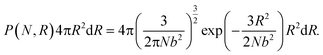 | (1) |
where b is the Kuhn length. Therefore, the probability of having a polymer strand between two certain junctions only depends on the distance between these two junctions. Periodic boundary conditions are applied when calculating all distances.
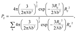
During the network forming process, one of the tetrafunctional junctions with at least one unoccupied functionality is randomly selected, followed by searching for all junctions with at least one unoccupied functionality and within the contour distance of the polymer strands from the first junction. Suppose i is the junction selected first, the probability of inserting a polymer strand between junctions i and j is calculated as
| |  | (2) |
The summation in the denominator is taken over all possible connections between the first selected junction and all junctions within the contour length. To simulate the real end-linked networks, we need to incorporate the possibility of having defects in the networks such as loops.
2,32–34 To allow the formation of the primary loops, we include the possibility of a “connection” being formed between junction
i and itself as long as this will not lead to more than four bonds on the junction. We set
Pij(
R < 1) =
Pij(
R = 1), and a prefactor is calculated to ensure that the summation of the probabilities over all possible choices of
R is equal to 1.
The Monte Carlo algorithm works as follows. A randomly distributed number is drawn from the interval [0, 1]. A junction j within the contour length of the first selected junction is randomly selected, and Pij is calculated. If the random number is smaller than Pij, the insertion of a polymer strand between these two junctions or the formation of a primary loop is accepted. If the random number is larger than the probability, the insertion is rejected. Another junction k within the contour length of the first junction i is selected next. We add  to Pik when considering the probability of insertion between i and k where
  is the summation of the probabilities of all previous unsuccessful attempts. The iteration continues until there is a successful insertion of a polymer strand or formation of a primary loop. Another type of defect, dangling end, may form if one junction with only one unoccupied functionality is selected and there is no possible connection between it and other junctions (including itself). One end of the bifunctional strand will be attached to that junction and the other remains disconnected to form a dangling end. For polymer strands inserted between two distinct junctions, beads are placed evenly on the straight line connecting the two junctions. For primary loops, beads are placed evenly on a ring with radius rloop = Nb/2π. To avoid the huge forces brought by the overlap of lines or rings, a small random fluctuation, which is a uniformly distributed random number drawn from the interval [−b/10, b/10] is added to each bead's coordinates.
Once all of the functionalities of one tetrafunctional junction are occupied, that junction is removed from the selection list. This process is repeated until 2n bifunctional polymer strands are inserted into the simulation box. Additionally, a small number of tracer particles are randomly placed in the networks to characterize the transport of small molecules through the networks. These tracer particles could represent gases that selectively adsorb into one domain or potentially ions moving through electrolytes. We keep the number of those unbonded tracer particles as small as 0.1% of the total number of particles in the systems so that the existence of those tracer particles will not affect the structure of network systems.
Unlike the Monte Carlo method adopted by Wang et al.,33 which grows the networks based on the topological distances between crosslinkers, our Monte Carlo method generates the networks using real-space distances, similar to the Monte Carlo method used by Gusev.35 Both the Wang et al. and Gusev's methods use parameters from real polymers, while our method is a more coarse-grained method using LJ units. As our goal for this work is to study the networks formed by tapered copolymers, our coarse-grained method aims to be computationally efficient to capture the morphologies of these networks. In section 3.1, we also compare the Monte Carlo method developed in this work with the reactive MD method previously used in our group2 to further validate this network generation method.
2.2 Tapered copolymer
In this work, tapered copolymer networks composed of monodisperse linear bifunctional polymer strands are studied. Strands with two different lengths N = 30 and N = 60 are used to build the systems. Following previous simulation studies,29,31,36,37 each strand is composed of a pure A block, a pure B block, and a gradient region between those two blocks. Inside the gradient region, the composition varies gradually from the pure A block to the pure B block. In other words, a site closer to the pure A block has a higher chance of placing an A monomer, and a site closer to the pure B block has a higher chance of placing a B monomer. The probability of placing a type A monomer at a certain site (s) along the polymer strand is calculated as| | 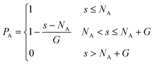 | (3) |
And the volume fraction of the pure A block is defined as| |  | (4) |
where NA is the length of the pure A block and G is the length of the gradient section. Fig. 1 shows how the probability of placing a monomer A changes with the location on the tapered copolymer strand schematically.
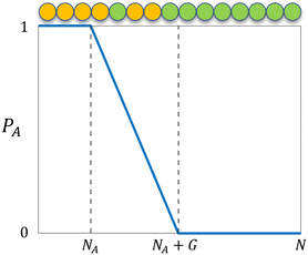 |
| | Fig. 1 The probability of placing a monomer A (PA) on a particular location of the tapered copolymer strand. NA is the length of the pure A block, G is the length of the gradient section, and N is the total length of the strand. | |
In this study, networks with different fA and G are studied. We treat the type A monomers as the minority domain, and networks with fA = 0.1, 0.15, 0.2 and 0.25 are tested; since each block of the copolymers are identical, we expect our systems to exhibit symmetric properties across fA = 0.5. Also, the maximum length of the gradient section of the networks is no longer than half of the strand length. Therefore, for networks with N = 30, we test systems with G = 0, 5, 10 and 15 and for networks with N = 60, we test systems with G = 0, 5, 10, 15, 20 and 30.
2.3 Network equilibration
Due to the random nature of our initial network generation, particles may overlap in the initial configurations. Therefore, the soft push-off method is used to remove any particle overlaps before switching to the Lennard-Jones (LJ) potential.38,39 The isothermal–isobaric (NPT) molecular dynamics simulations are then used to equilibrate the network systems. All junctions, monomers (type A and B) and tracer particles (I) are modeled as LJ beads. Nonbonded interactions are modeled using the cut-and-shifted LJ potential,| | 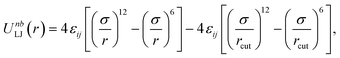 | (5) |
where the cutoff distance rcut = 2.5σ. The LJ interaction parameters between all species are set to be εij = 1.0, except that εAB = 0.4 to induce phase separation, and εBI = 0.1 so that the tracer particles only prefer the minority domain of the network (type A monomers). Bonding is maintained through a harmonic bond potential| | 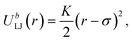 | (6) |
where K = 400(ε/σ2). The system temperature is kept at T = 0.7 and the pressure is maintained at P = 1.0 using the Nose–Hoover thermostat and barostat. The integration time step for the velocity-Verlet algorithm is set to be 0.002τ, where τ is the unit LJ time. For the N = 30 and the N = 60 network systems, the NPT MD algorithms are run 100![[thin space (1/6-em)]](https://www.rsc.org/images/entities/char_2009.gif) 000τ and 120000τ respectively, to ensure a full equilibration of the network structures. All molecular dynamics simulations are performed using the LAMMPS package,40,41 and the visualizations and cluster analyses were performed using OVITO.42
000τ and 120000τ respectively, to ensure a full equilibration of the network structures. All molecular dynamics simulations are performed using the LAMMPS package,40,41 and the visualizations and cluster analyses were performed using OVITO.42
3 Results
3.1 Validation of the network generation method
We compare the primary loop fractions and the shear moduli of networks generated by the Monte Carlo (MC) method introduced in section 2.1 and networks generated by the reactive molecular dynamics (MD) method2 to validate the network generation method. The primary loop fraction (f1) is defined as the ratio of the number of junctions that contain primary loops relative to the total number of junctions. Previous work has shown that the primary loop fraction is an essential indicator of the defect density in the network.33,34 The primary loop fractions of networks with three different strand lengths, N = 5, 10 and 20 are compared in Table 1, with the same system size.
Table 1 Primary loop fraction (f1) and shear moduli (μ) comparison between networks generated by the Monte Carlo (MC) and the molecular dynamics (MD) methods
| Strand length |
f
1
|
μ
|
| MC |
MD |
MC |
MD |
| 5 |
0.15 |
0.16 |
0.199 ± 0.0452 |
0.129 ± 0.0018 |
| 10 |
0.13 |
0.13 |
0.049 ± 0.0031 |
0.055 ± 0.0006 |
| 20 |
0.08 |
0.09 |
0.033 ± 0.0014 |
0.041 ± 0.0006 |
The primary loop fractions of the polymer networks generated by these two methods agree well. The shear modulus (μ) of each network is obtained by performing the uniaxial tension in one direction of the network at a constant true strain rate ![[small epsi, Greek, dot above]](https://www.rsc.org/images/entities/i_char_e0a1.gif) t while keeping the pressure of the other two directions constant. The strain rate t is chosen to be 2.5 × 10⁻⁵ as in our group's previous work.2 The shear modulus is then achieved by fitting the stress–strain curve to the Gent model43
t while keeping the pressure of the other two directions constant. The strain rate t is chosen to be 2.5 × 10⁻⁵ as in our group's previous work.2 The shear modulus is then achieved by fitting the stress–strain curve to the Gent model43
| |  | (7) |
where
σ is the component of the stress tensor in the deformed direction,
λ stands for the change in length in the deformed direction and is defined as
λ =
L(
t)/
L(0),
J1 =
λ2 + 2
λ−1 − 3 and
Jm is a fitting parameter. From
Table 1, only the
N = 5 systems exhibit a statistically-significant difference in the measured moduli from the two network generation methods. We hypothesize this discrepancy is due to the assumption of Gaussian chain statistics when we form the network, as the
N = 5 chains are too short to exhibit Gaussian statistics. With relatively long strand lengths (the
N = 10 and
N = 20 systems) we see a good agreement in the shear moduli. As the Monte Carlo method is more efficient at constructing the initial configurations and the networks studied in this work have relatively long strand lengths (
N = 30 and
N = 60), we proceed to use the MC method to build the initial configurations in this study.
3.2 Network microstructure
We first characterize how the gradient in the block copolymer affects the percolation of the minority domain at different minority domain compositions fA. Cross-sectional images of the minority domain in equilibrated networks at each fraction of the minor domain (fA) and gradient section length (G) are obtained via OVITO42 and presented in Fig. 2. The cluster sizes and their ability to form percolating domains depends on both fA and G. For systems with both low fractions of the minority domain and short gradient sections (e.g., fA = 0.1 and G = 0), disconnected, small clusters are spread within the network. In contrast, system-spanning clusters are formed throughout the network for systems with high fractions of the minority domain or long gradient sections.
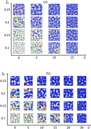 |
| | Fig. 2 Cross-sectional images of clusters formed by the minority domain (type A monomers) of the networks with the strand length (a) N = 30 and (b) N = 60. Different colors represent different clusters, and the dark blue cluster is the largest cluster in the box. | |
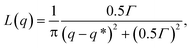
Structure factors are computed on the minority domain to characterize the long-range order of the structures (inset of Fig. 3(a)). Lorentzian functions are then used to fit the low-q peak of the structure factor curves,
| |  | (8) |
where
q* is the location of the peak and
Γ is a fitting parameter. The domain spacing
d = 2π/
q* can be therefore determined from the fitting.
Fig. 3 shows how domain spacing changes as a function of the gradient length for each strand length and fraction of the minority domain. Nearly all curves show a non-monotonic trend that the domain spacing increases with
G at low
G. However, once
G exceeds a critical value, the domain spacing drops with increasing
G. We will attempt to explain this non-monotonic trend using the cluster analyses. At fixed gradient length
G, the domain spacing generally increases with
fA. In the limit of large
G, the domain spacing becomes less sensitive to the value of
fA. Moreover, to examine the influence of the initial configuration on the results, we chose
N = 60,
fA = 0.1 systems with different
G, generated three configurations for each system and calculated the structure factors. We verified that the domain spacing calculated is consistent for each system, with a maximum deviation less than 1
σ.
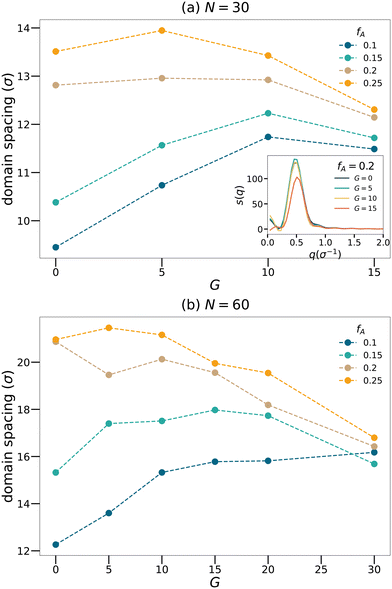 |
| | Fig. 3 Domain spacing curves for the (a) N = 30 and (b) N = 60 network systems. Inset of the panel (a) shows sample structure factor curves for network systems with N = 30 and fA = 0.2. | |
To further quantify the percolation phenomena, cluster analyses of the minority domain (type A monomers) are performed using tools in OVITO.42 Two particles are considered connected if their distance is within the cutoff distance chosen to be 1.1σ in this analysis. If one continuous path connecting the two particles exists, the two particles belong to the same cluster. We count the sizes as the number of monomers comprising the largest cluster and the second-largest cluster within each network as shown in Fig. 4, and the sizes of the clusters are normalized by the total number of type A monomers in each system. Generally, the dimensions of the largest clusters grow with G, and the size of the second-largest clusters decreases once the largest cluster spans the system. Comparing Fig. 3 and 4, the critical G of the domain spacing curves almost occurs at the same location as for the percolation transition. Before a continuous giant cluster forms, increasing the gradient length grows the domain spacing but after a continuous cluster occupies the network, the domain spacing decreases with the increasing G. For all values of fA considered here, we are able to observe an apparent percolation of the largest cluster. For larger values of fA, only a small gradient is required to observe percolation, while larger gradient regions are required for fA = 0.1 and 0.15. This result shows that engineering the polymer strands that form the network allows the system to reach percolation at small values of fA.
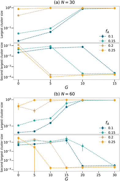 |
| | Fig. 4 Cluster analyses performed on the minority domain of the equilibrated networks with the strand length (a) N = 30 and (b) N = 60 to count the sizes of largest and second largest clusters. The sizes of the clusters are normalized by the total number of type A monomers in each system. | |
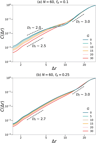
Moreover, fractal analyses are performed to investigate how the minority domain fills the simulation boxes. We estimate the fractal dimension of the minority domain (type A monomers) using the correlation dimension.44 The correlation integral C(Δr) is calculated by44
| | 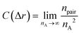 | (9) |
where
npair is the number of pairs of type A monomers whose distances are less than Δ
r and
nA is the number of type A monomers in the system. The scaling of the log–log plot of
C(Δ
r)
vs. Δ
r reports an estimation of the fractal dimension. Fractal analyses are performed on
N = 60 networks with two different fractions of the minority domain and various gradient section lengths as shown in
Fig. 5. For systems with small values of
fA and
G, the curves cannot be fit with a single fractal dimension and therefore suggest a multifractal behavior. At a small length scale, the fractal dimensions of these systems are less than 2.5, which is the critical fractal dimension for three-dimensional percolation.
1,45,46 Therefore, the minority domain does not percolate in three dimensions, which agrees with the results from the visualization and the cluster analyses. While for network systems with larger values of
fA and
G, an approximately uniform fractal dimension larger than 2.5 is observed across different length scales, suggesting a self-similar and three-dimensional percolating behavior for these systems.
 |
| | Fig. 5 Fractal analyses performed on the minority domain in the N = 60, (a) fA = 0.1 and (b) fA = 0.25 network systems with various gradient section lengths (G). The scaling of the log–log plots reports an estimation of the fractal dimension. Black dashed lines are eye-guides with different scaling. | |
We also calculate the correlation length of clusters formed by the minority domain using
| |  | (10) |
where
Rgi is the radius of gyration and
Si is the size of each cluster
i.
46,47 As shown in
Fig. 6, for each
fA, there is a gradient length
G where the correlation length
ξ approaches the size of the simulation box (∼40
σ), which is a feature of the percolation transition. The fractal analyses and the calculation of the correlation length further support that by tuning the gradient section lengths (
G), tapered copolymer network systems are able to reach three-dimensional percolation at small values of
fA.
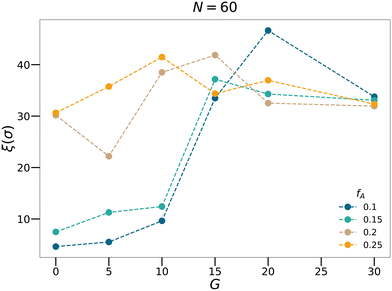 |
| | Fig. 6 The correlation length calculated for the N = 60 systems with various minority domain fractions fA and gradient section lengths G. | |
3.3 Transport dynamics of the networks
To explore the transport dynamics within the networks, the mean square displacement (MSD) of the tracer particles placed in the networks with different strand lengths (N), fractions of the minor domain (fA) and gradient section lengths (G) is shown in Fig. 7. The MSD curves exhibit qualitatively similar behaviors at both strand lengths. For networks with high fractions of the minor domain (fA = 0.2 or fA = 0.25), the mean square displacement is linearly proportional to time on the log–log plots and is almost independent of the length of the gradient section. While for networks with low fractions of the minor domain (fA = 0.1 or fA = 0.15), MSD increases as a function of G gradually. In particular, for systems with low fractions of the minor domain and short gradient section lengths (e.g., fA = 0.1 and G = 0), the MSD on the time scales sampled remains subdiffusive as the tracers are trapped in isolated domains. The diffusion behavior of these tracer particles corresponds well to the structures of the minority domain in each network and appears to be highly mobile in samples with percolating structures. It is interesting to note that the mobility is only weakly dependent on fA for large G, as percolation appears to be the most important aspect for maintaining highly mobile penetrants and not the size or tortuosity of the domains.
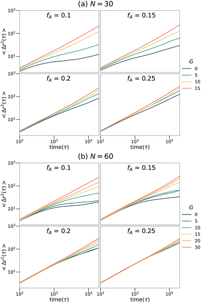 |
| | Fig. 7 Mean square displacement curves of tracers selective for the minor phase in the (a) N = 30 and (b) N = 60 network systems. | |
4 Conclusions
We show that tapered copolymer networks with different strand lengths, fractions of the minority domain and gradient region lengths have different equilibrium structures. Gradient section lengths can be tuned to control the domain spacing and percolation transitions of the clusters formed by the minority domain. Based on the equilibrium structures, the diffusion of non-charged tracer particles will have two modes. For networks with low fA and G, tracer particles are trapped in isolated domains so they undergo subdiffusion. For networks with high fA or G, the minority domain forms continuous structures. As a result, the tracer particles can diffuse freely within the networks. Future work will consider how the bond rigidity affects the percolation phenomena.
Conflicts of interest
There are no conflicts to declare.
Acknowledgements
The authors acknowledge support from the Office of Naval Research via ONR-N00014-17-1-2056. Computational resources were made available through XSEDE Award TG-DMR150034. The authors thank Ziyu Ye and Amruthesh Thirumalaiswamy for the helpful discussions.
Notes and references
-
M. Rubinstein and R. H. Colby, Polymer Physics, OUP Oxford, Oxford, 2003 Search PubMed.
- Z. Ye and R. A. Riggleman, Macromolecules, 2020, 53, 7825–7834 CrossRef CAS.
- S. P. O. Danielsen, H. K. Beech, S. Wang, B. M. El-Zaatari, X. Wang, L. Sapir, T. Ouchi, Z. Wang, P. N. Johnson, Y. Hu, D. J. Lundberg, G. Stoychev, S. L. Craig, J. A. Johnson, J. A. Kalow, B. D. Olsen and M. Rubinstein, Chem. Rev., 2021, 121, 5042–5092 CrossRef CAS PubMed.
- Y. Gu, J. Zhao and J. A. Johnson, Angew. Chem., Int. Ed., 2020, 59, 5022–5049 CrossRef CAS PubMed.
- D. Montarnal, M. Capelot, F. Tournilhac and L. Leibler, Science, 2011, 334, 965–968 CrossRef CAS PubMed.
- J. Gong, Y. Katsuyama, T. Kurokawa and Y. Osada, Adv. Mater., 2003, 15, 1155–1158 CrossRef CAS.
- M. A. Haque, T. Kurokawa and J. P. Gong, Polymer, 2012, 53, 1805–1822 CrossRef CAS.
- C. N. Walker, K. C. Bryson, R. C. Hayward and G. N. Tew, ACS Nano, 2014, 8, 12376–12385 CrossRef CAS.
- A. J. Meuler, M. A. Hillmyer and F. S. Bates, Macromolecules, 2009, 42, 7221–7250 CrossRef CAS.
- G. Jo, H. Ahn and M. J. Park, ACS Macro Lett., 2013, 2, 990–995 CrossRef CAS PubMed.
- W.-S. Young, W.-F. Kuan and T. H. Epps, J. Polym. Sci., Part B: Polym. Phys., 2014, 52, 1–16 CrossRef CAS.
- M. A. Morris, H. An, J. L. Lutkenhaus and T. H. Epps, ACS Energy Lett., 2017, 2, 1919–1936 CrossRef CAS.
- T. Ichikawa, M. Yoshio, A. Hamasaki, J. Kagimoto, H. Ohno and T. Kato, J. Am. Chem. Soc., 2011, 133, 2163–2169 CrossRef CAS PubMed.
- L. Yan, C. Rank, S. Mecking and K. I. Winey, J. Am. Chem. Soc., 2020, 142, 857–866 CrossRef CAS PubMed.
- E. J. W. Crossland, M. Kamperman, M. Nedelcu, C. Ducati, U. Wiesner, D. M. Smilgies, G. E. S. Toombes, M. A. Hillmyer, S. Ludwigs, U. Steiner and H. J. Snaith, Nano Lett., 2009, 9, 2807–2812 CrossRef CAS PubMed.
- F. S. Bates and G. H. Fredrickson, Phys. Today, 1999, 52, 32–38 CrossRef CAS.
- D. Zeng, A. Ribbe and R. C. Hayward, Macromolecules, 2017, 50, 4668–4676 CrossRef CAS.
- S. Panyukov and M. Rubinstein, Macromolecules, 1996, 29, 8220–8230 CrossRef CAS.
- M. Haraszti, E. Tóth and B. Iván, Chem. Mater., 2006, 18, 4952–4958 CrossRef CAS.
- M. Seo, M. A. Amendt and M. A. Hillmyer, Macromolecules, 2011, 44, 9310–9318 CrossRef CAS.
- Y. Chen, D. Yuan and C. Xu, ACS Appl. Mater. Interfaces, 2014, 6, 3811–3816 CrossRef CAS.
- D. Zeng and R. C. Hayward, Macromolecules, 2019, 52, 2642–2650 CrossRef CAS.
- J. M. Widin, A. K. Schmitt, A. L. Schmitt, K. Im and M. K. Mahanthappa, J. Am. Chem. Soc., 2012, 134, 3834–3844 CrossRef CAS.
- I. Lee and F. S. Bates, Macromolecules, 2013, 46, 4529–4539 CrossRef CAS.
- C. N. Walker, J. M. Sarapas, V. Kung, A. L. Hall and G. N. Tew, ACS Macro Lett., 2014, 3, 453–457 CrossRef CAS PubMed.
- D. Zeng, R. Gupta, E. B. Coughlin and R. C. Hayward, ACS Appl. Polym. Mater., 2020, 2, 3282–3290 CrossRef CAS.
- R. Roy, J. K. Park, W.-S. Young, S. E. Mastroianni, M. S. Tureau and T. H. Epps, Macromolecules, 2011, 44, 3910–3915 CrossRef CAS.
- W.-F. Kuan, R. Roy, L. Rong, B. S. Hsiao and T. H. Epps, ACS Macro Lett., 2012, 1, 519–523 CrossRef CAS PubMed.
- J. R. Brown, S. W. Sides and L. M. Hall, ACS Macro Lett., 2013, 2, 1105–1109 CrossRef CAS PubMed.
- W.-F. Kuan, R. Remy, M. E. Mackay and T. H. Epps, III, RSC Adv., 2015, 5, 12597–12604 RSC.
- Y. Seo, J. R. Brown and L. M. Hall, Macromolecules, 2015, 48, 4974–4982 CrossRef CAS.
- H. Zhou, J. Woo, A. M. Cok, M. Wang, B. D. Olsen and J. A. Johnson, Proc. Natl. Acad. Sci. U. S. A., 2012, 109, 19119–19124 CrossRef CAS.
- R. Wang, A. Alexander-Katz, J. A. Johnson and B. D. Olsen, Phys. Rev. Lett., 2016, 116, 188302 CrossRef PubMed.
- M. Zhong, R. Wang, K. Kawamoto, B. D. Olsen and J. A. Johnson, Science, 2016, 353, 1264–1268 CrossRef CAS PubMed.
- A. A. Gusev, Macromolecules, 2019, 52, 3244–3251 CrossRef CAS.
- W. G. Levine, Y. Seo, J. R. Brown and L. M. Hall, J. Chem. Phys., 2016, 145, 234907 CrossRef PubMed.
- Y. Seo, J. R. Brown and L. M. Hall, ACS Macro Lett., 2017, 6, 375–380 CrossRef CAS PubMed.
- R. Auhl, R. Everaers, G. S. Grest, K. Kremer and S. J. Plimpton, J. Chem. Phys., 2003, 119, 12718–12728 CrossRef CAS.
- Y. R. Sliozberg and J. W. Andzelm, Chem. Phys. Lett., 2012, 523, 139–143 CrossRef CAS.
- S. Plimpton, J. Comput. Phys., 1995, 117, 1–19 CrossRef CAS.
- A. P. Thompson, H. M. Aktulga, R. Berger, D. S. Bolintineanu, W. M. Brown, P. S. Crozier, P. J. in ‘t Veld, A. Kohlmeyer, S. G. Moore, T. D. Nguyen, R. Shan, M. J. Stevens, J. Tranchida, C. Trott and S. J. Plimpton, Comput. Phys. Commun., 2022, 271, 108171 CrossRef CAS.
- A. Stukowski, Modell. Simul. Mater. Sci. Eng., 2010, 18, 015012 CrossRef.
- A. N. Gent, Rubber Chem. Technol., 1996, 69, 59–61 CrossRef CAS.
- P. Grassberger and I. Procaccia, Phys. D, 1983, 9, 189–208 CrossRef.
-
D. Stauffer, A. Coniglio and M. Adam, Polymer Networks, Springer Berlin Heidelberg, Berlin, Heidelberg, 1982, vol. 44, pp. 103–158 Search PubMed.
-
D. Stauffer and A. Aharony, Introduction to percolation theory, Taylor & Francis, London, 1994 Search PubMed.
- A. Ghosh, Z. Budrikis, V. Chikkadi, A. L. Sellerio, S. Zapperi and P. Schall, Phys. Rev. Lett., 2017, 118, 148001 CrossRef PubMed.
|
| This journal is © The Royal Society of Chemistry 2023 |
Click here to see how this site uses Cookies. View our privacy policy here. 
 and
Robert A.
Riggleman
and
Robert A.
Riggleman


 to Pik when considering the probability of insertion between i and k where
  is the summation of the probabilities of all previous unsuccessful attempts. The iteration continues until there is a successful insertion of a polymer strand or formation of a primary loop. Another type of defect, dangling end, may form if one junction with only one unoccupied functionality is selected and there is no possible connection between it and other junctions (including itself). One end of the bifunctional strand will be attached to that junction and the other remains disconnected to form a dangling end. For polymer strands inserted between two distinct junctions, beads are placed evenly on the straight line connecting the two junctions. For primary loops, beads are placed evenly on a ring with radius rloop = Nb/2π. To avoid the huge forces brought by the overlap of lines or rings, a small random fluctuation, which is a uniformly distributed random number drawn from the interval [−b/10, b/10] is added to each bead's coordinates.


