
 Open Access Article
 This Open Access Article is licensed under a Creative Commons Attribution-Non Commercial 3.0 Unported Licence
Upcycling natural Limestone waste for thermochemical energy storage by utilising tailored CaZrO3 nanoadditives†
Rehan
Anwar
a,
Jan
Navrátil
 bc,
Rajani K.
Vijayaraghavan
d,
Patrick J.
McNally
d,
Michal
Otyepka
be,
Piotr
Błoński
b and
M. Veronica
Sofianos
*a
bc,
Rajani K.
Vijayaraghavan
d,
Patrick J.
McNally
d,
Michal
Otyepka
be,
Piotr
Błoński
b and
M. Veronica
Sofianos
*a
aSchool of Chemical and Bioprocess Engineering, University College Dublin, Belfield, Dublin 4, Ireland. E-mail: mvsofianou@gmail.com
bRegional Centre of Advanced Technologies and Materials, Czech Advanced Technology and Research Institute (CATRIN), Palacký University, Šlechtitelů 27, 783 71, Olomouc, Czech Republic
cDepartment of Physical Chemistry, Faculty of Science, Palacký University, 17. listopadu 1192/12, 779 00 Olomouc, Czech Republic
dSchool of Electronic Engineering, Dublin City University, Glasnevin, Dublin 9, Ireland
eIT4Innovations, Technical University of Ostrava, 708 00 Ostrava-Poruba, Czech Republic
First published on 3rd March 2023
Abstract
The development of long-term renewable energy storage systems is crucial for decarbonising the energy sector and enabling the transition to a sustainable energy future. Thermochemical energy storage (TCES) systems are well suited for long-term renewable energy storage as the materials used in these systems have high energy densities, and long storage duration. Among the plethora of TCES materials, calcium carbonate (Limestone) is of particular interest since it exhibits a high enthalpy of reaction, and it is earth-abundant. The main problem with Limestone inhibiting its commercial application for long-term renewable energy storge is its deteriorating cycling performance after several energy charge/discharge cycles. In this study, two CaZrO3 nanoadditives with two different Ca![[thin space (1/6-em)]](https://www.rsc.org/images/entities/char_2009.gif) :Zr ratios and tailored oxygen vacancies were synthesised by a precipitation method, and mixed with Limestone waste at three weight concentrations (5, 10 and 20 wt%). Their phase, chemical state and morphology were determined by XRD, XPS and TEM, respectively. The cycling performance of the mixture samples was determined through thermogravimetric analysis. The best performing sample was the one mixed with 20% CaZrO3 nanoadditives, which contained a large number of oxygen vacancies and thus had enhanced ionic conductivity, as confirmed by density functional theory (DFT) calculations. This sample exhibited the best effective conversion and the highest energy density values of 0.7 and 2640 kJ kg−1, respectively, after 40 cycles.
:Zr ratios and tailored oxygen vacancies were synthesised by a precipitation method, and mixed with Limestone waste at three weight concentrations (5, 10 and 20 wt%). Their phase, chemical state and morphology were determined by XRD, XPS and TEM, respectively. The cycling performance of the mixture samples was determined through thermogravimetric analysis. The best performing sample was the one mixed with 20% CaZrO3 nanoadditives, which contained a large number of oxygen vacancies and thus had enhanced ionic conductivity, as confirmed by density functional theory (DFT) calculations. This sample exhibited the best effective conversion and the highest energy density values of 0.7 and 2640 kJ kg−1, respectively, after 40 cycles.
Introduction
Long-term energy storage is essential if renewable energy is to replace the use of fossil fuels and meet global energy demands.1 Due to its intermittent nature, reliable and continuous renewable power-to-grid supply cannot be ensured, therefore long-term energy storage is crucial. There are a number of long-term energy storage systems that can address the renewable energy intermittency, the most popular being flow batteries,2 pumped hydro energy storage,3 and thermal energy storage. Thermal energy storage (TES) is considered one of the most promising energy storage systems due to its affordability and efficiency.4,5There are three types of TES systems based on their energy storage mode: sensible heat storage (SHS), latent heat storage (LHS) and thermochemical energy storage (TCES).6,7 SHS uses temperature changes of a material to store heat energy. SHS systems have low energy densities (72–108 kJ kg−1) and limited storage duration due to thermal losses.8 In LHS systems, phase change materials are used to store heat energy. When these materials change their phase, they absorb/release heat. LHS systems possess relatively larger energy densities (108–360 kJ kg−1) to SHS, but have a limited storage duration associated with thermal losses.9 TCES systems utilize reversible chemical reactions for heat energy storage.10 TCES is the most promising TES system as the materials used have higher energy densities (1800–3600 kJ kg−1) in comparison to the other two systems and long-term storage duration.11
As mentioned before, TCES systems utilize reversible chemical reactions for storing heat. During their endothermic reactions, heat is stored while heat is released during their reverse exothermic reactions.12 Metal carbonates,13–16 hydrides,17–20 and hydroxides12,21 are commonly used materials for TCES systems.22 Calcium carbonate (CaCO3), also known as Limestone, has a high enthalpy of (calcination/carbonation) reaction (ΔH890°C = 165.7 kJ), it is easy to handle and transport, has a high energy storage density (>1000 kJ kg−1) and is earth-abundant, making it a very attractive candidate for storing renewable energy long-term.4,23,24 CaCO3 dissociates into CaO and CO2 by absorbing heat (calcination), and can theoretically release the same amount of heat during the reverse reaction (carbonation).25,26
| CaCO3 ↔ CaO + CO2 ΔH890°C = 165.7 kJ |
Unfortunately, Limestone has very slow reaction kinetics during charge/discharge (cycling), and its energy storage capacity degrades upon consecutives energy charge/discharge cycles. It is believed that these drawbacks are related to sintering phenomena, and poor ionic mobility of Ca2+, O2− and CO32− at high temperatures.30–32
According to the literature, a plethora of additives have been used as an effective way to enhance the cycling performance of Limestone, including Al2O3,33–35 SiO2,36–38 and ZrO2.27–29,39–41 Among these additives, ZrO2 has been the most promising. In most published studies it was reported, that ZrO2 converts to CaZrO3 during cycling (Table 1), stating that this ternary oxide plays the key role in improving the cycling performance of Limestone.
CaZrO3 is a perovskite with a high meting point (2345 °C), small thermal expansion coefficient, high strength, excellent corrosion resistance against alkali oxides, and is chemically and thermally stable at high temperatures.42 Due to its perovskite structure, it possess a high ionic conductivity, promoting ionic diffusion during catalytic reactions.43 CaZrO3 has been reported to have been used for catalytic ozonation, CO2 capturing, sensing humidity, and in dielectric applications.43–46
To the best of our knowledge, this is the first study to use tailored CaZrO3 nanoadditives for upcycling natural Limestone waste for thermochemical energy storage. The CaZrO3 nanoparticles were synthesized using a wet precipitation method and were systematically characterized using both experimental and computational methods. Their morphology, specific surface area and chemical composition were determined by SEM/TEM, BET analysis, and XRD/XPS respectively. Their ionic conductivity was studied theoretically in the framework of DFT, determining energy barriers for their transport in the studied systems. These tailored nanoparticles were mixed with Limestone waste in three different weight percentages (5, 10 and 20 wt%). How the difference in ionic conductivity, particle size, specific surface area and weight concentration of the CaZrO3 nanoadditives influence the cycling stability and thermochemical energy storage properties of Limestones was reported.
Experimental
Synthesis of CaZrO3 nanoadditives
CaZrO3 nanoparticles were synthesized using a wet precipitation method. Specifically, two samples, CaZrO3-I and CaZrO3-II, were prepared using two different stoichiometric ratios of Ca to Zr as seen in (Table 2). Stoichiometrically calculated amounts of CaCl2·2H2O (>99%, Honeywell) and ZrOCl2·8H2O (98%, ACROS ORGANICS) were dissolved in ethanol, and then mixed together under continuous magnetic stirring to obtain a uniform solution. Specific amounts of NaOH (>97%, SIGMA-ALDRICH) were added to the above solution to obtain an overall molarity of 0.5 M for the final solution. The solution was then kept at 50 °C for 24 h under constant stirring. The resulting white precipitates were collected by centrifugation, dried in an oven at 110 °C for 24 h, and then further calcined at 1000 °C for 3.5 h with a 3 °C min−1 heating rate Fig. 1.| Sample ID | Stoichiometric ratio (Ca:Zr) |
|---|---|
| CaZrO3-I | 1:1 |
| CaZrO3-II | 0.9:1 |
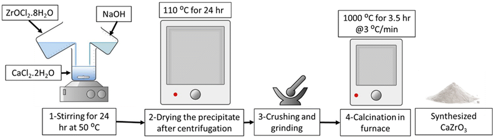 | ||
| Fig. 1 Illustration of the CaZrO3 nanoparticle synthesis method. | ||
CaZrO3/Limestone sample preparation
The CaZrO3/Limestone samples were prepared by physically mixing CaZrO3 nanoparticles and Limestone waste (Bennettsbridge Limestone Quarries, Ireland) in three different weight percentages (Table 3) using a mortar and pestle. Limestone waste was heated at 500 °C for two hours prior to further use in order to remove any impurities. More details can be found in the thermal analysis of natural Limestone section.| Sample description | Sample IDs | |
|---|---|---|
| Before cycling | After cycling | |
| 100% Limestone waste | Lim BBL | 40_Lim BBL |
| 5% CaZrO3-I + 95% Limestone waste | 5R1 | 40_5R1 |
| 10% CaZrO3-I + 90% Limestone waste | 10R1 | 40_10R1 |
| 20% CaZrO3-I + 80% Limestone waste | 20R1 | 40_20R1 |
| 5% CaZrO3-II + 95% Limestone waste | 5R0.9 | 40_5R0.9 |
| 10% CaZrO3-II + 90% Limestone waste | 10R0.9 | 40_10R0,9 |
| 20% CaZrO3-II + 80% Limestone waste | 20R0.9 | 40_20R0.9 |
Materials characterization
Scanning electron microscopy
A Zeiss Sigma 300 scanning electron microscope (SEM) was used for morphological observations. SEM specimens were prepared by placing a small amount of powder onto carbon tape and then coating them with a 4 nm layer of platinum to produce a conductive layer and reduce charging during SEM imaging. EDS mapping was done on a Hitachi Regulus 8230 Field Emission Gun Scanning Electron Microscope (FEGSEM) coupled with an Oxford Astec 170 EDS and manipulated by the Aztec software.Transmission electron microscopy
A high-resolution transmission electron microscope (HR-TEM) was used to observe the CaZrO3 nanoparticles using a Tecnai 20 TEM with an acceleration voltage of 200 kV. TEM samples were prepared on copper grids by placing few drops of suspension (CaZrO3 nanoparticles and ethanol) and dried under an IR lamp for 20–30 seconds.Brunauer–Emmett–Teller method
Specific surface area calculations for all samples were performed by applying nitrogen (N2) adsorption at 77 K using a Micromeritics Gemini VII system (Micromeritics, Nor-cross, GA, USA), and employing the Brunauer–Emmett–Teller (BET) multi-point method using the relative pressures between 0.05 and 0.30 bar. All samples were outgassed at 200 °C under a nitrogen atmosphere prior to their N2 adsorption analysis.X-ray photoelectron spectroscopy
The CaZrO3 samples were also tested by X-ray photoelectron spectroscopy (XPS), using a Kratos AXIS Ultra DLD X-ray photoelectron spectrometer in ultra-high vacuum equipped with an Al Kα X-ray source (1486.7 eV). The data was analyzed using the Casa XPS software and calibrated using the surface adventitious C 1s peak at 284.5 eV.Density functional theory calculations
All calculations in this work were performed in the DFT framework, as implemented in the plane-wave Vienna ab initio simulation package (VASP).47–50 The basis set was limited to plane waves with a maximum kinetic energy of 400 eV. The electron–ion interactions were treated by the projected augmented wave (PAW) method.51,52 The electronic exchange and correlation effects were handled at the generalized-gradient approximation (GGA) level using the functional of Perdew, Burke and Ernzerhof (PBE).53,54 Grimme's zero-damping DFT-D3 method was used to account for London dispersion interactions.55 The electronic degrees of freedom were relaxed by a preconditioned conjugate gradient algorithm with an electronic energy convergence threshold set at 10−6 eV. For Brillouin zone sampling, after convergence tests (Table S1, ESI†), a Γ-centred 2 × 2 × 2 k-point mesh was used.Initially, two structures of CaZrO3 shown in Fig. 2, orthorhombic and cubic, were considered. Since the former is ∼0.2 eV per atom more stable than the latter, it was used in further calculations.
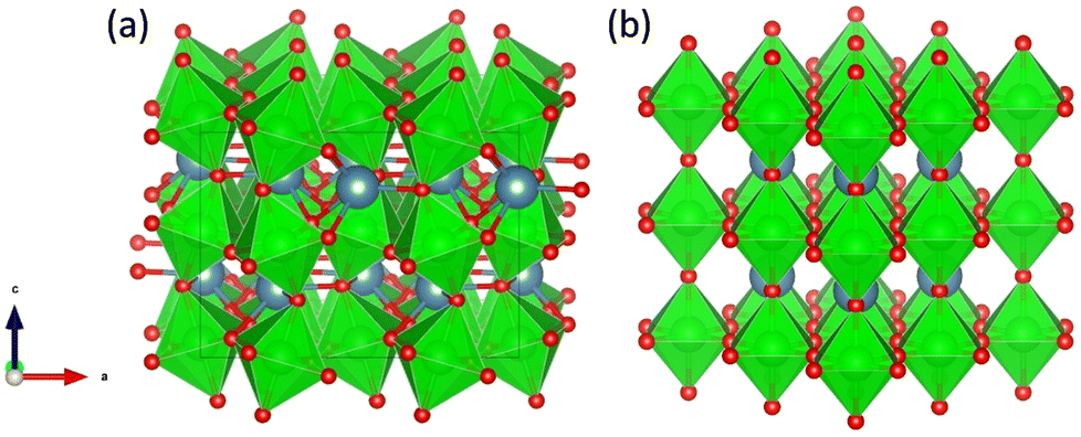 | ||
| Fig. 2 Orthorhombic (a) and cubic (b) structure of CaZrO3. Ca, Zr and O atoms are represented by blue, green and red spheres, respectively. ZrO6 octahedra are indicated in green. | ||
The structures were optimized, including the lattice constants, by the conjugate gradient algorithm until all forces acting on the atoms were reduced to less than 0.02 eV Å−1.
Structures were visualized using VESTA56 or Speck.57 All other calculation details can be found in Section S2 (ESI†).
Thermogravimetric analysis
Thermogravimetric analysis of Limestone was performed on a TA Q500 instrument. For this measurement, 30–35 mg of powder Limestone was placed in a Pt crucible. Firstly, the sample was heated from room temperature to 1000 °C under a N2 flow (100 mL min−1) with a 20 °C min−1 and was kept isothermal for 20 min under a CO2/N2 flow (CO2 at 90 mL min−1 and N2 at 10 mL min−1) and cooled down to room temperate with a 20 °C min−1 cooling rate under the same atmosphere.Calcination/carbonation cycling and heat storage performance
Calcination and carbonation cycles were performed using a thermogravimetric analyzer Q500 by TA instruments at a constant temperature of 884 °C. The calcination step was performed under a 100 mL min−1 N2 flow with 10 min dwell time, whereas the carbonation step took place under a mixture of 90 mL min−1 CO2 and 10 mL min−1 N2 flow with 20 min dwell time. At the start of the cycling measurements, all samples were heated from room temperature to 884 °C under a N2 flow (100 mL min−1) with a 20 °C min−1 heating rate. At the end of the cycling, all samples were cooled down to room temperature under a CO2/N2 flow (CO2 at 90 mL min−1 and N2 at 10 mL min−1) with a 20 °C min−1 cooling rate.The heat storage performance of all samples was evaluated by the effective conversion, and the heat storage density. The effective conversion, Xef,N, represents the ratio of the mass of CaO that has reacted during each carbonation step (cycle) to the total mass of the sample before the carbonation, as defined by eqn (1):
 | (1) |
Heat storage density, Eg,N, in kJ kg−1, denotes the maximum heat that can be released per unit mass of the samples during each carbonation reaction, as defined by eqn (2):
 | (2) |
kJ mol−1.
Results and discussion
Phase and morphological observations and specific surface area calculations of CaZrO3
XRD patterns of the CaZrO3-I and CaZrO3-II samples are presented in Fig. 3. The predominant phase corresponds to CaZrO3 (PDF 96-153-2748). It is suspected that due to the higher stoichiometric ratio of Zr to Ca in the CaZrO3-II sample, a secondary phase of ZrO2 (PDF 96-900-9052) with peaks identified at 30° and 35° 2θ is present.58 A CaO peak for the CaZrO3-I sample at 30° 2θ is represent in its diffraction pattern due to unreacted CaO (PDF 96-900-6747).59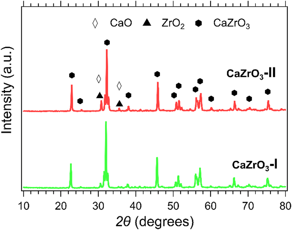 | ||
| Fig. 3 XRD patterns of CaZrO3-l (green) and CaZrO3-ll (red). Peaks of CaO are represented with the white diamond marker and ZrO2 with the black triangle marker. | ||
The as-synthesised CaZrO3 nanoparticles can be observed in the SEM (Fig. 4(a) and (c)) and TEM (Fig. 4(b) and (d)) micrographs. It is noticeable that the size of the nanoparticles is polydisperse in both CaZrO3 samples. As the final synthesis step was calcination of the dried precipitates at 1000 °C, sintering of some nanoparticles can be observed in both samples. Despite this, all the CaZrO3 particles are still in the nanometre range.
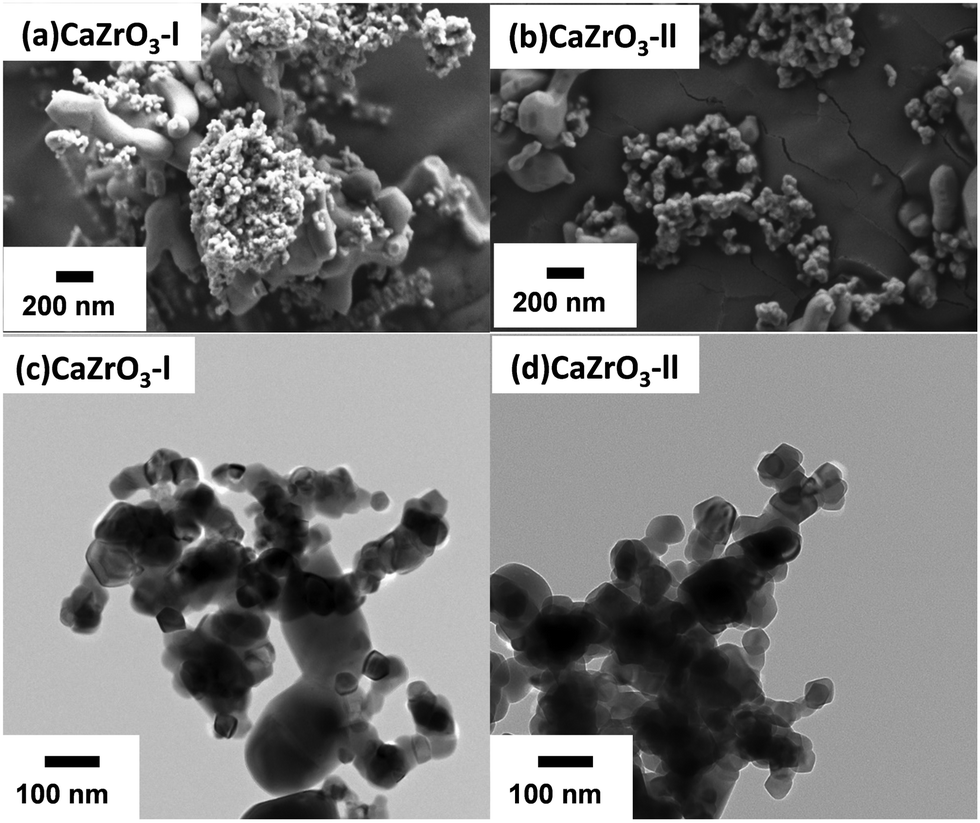 | ||
| Fig. 4 SEM (a), (b) and TEM (c), (d) images of CaZrO3-l and CaZrO3-ll. | ||
The BET surface area was 8.99 ± 0.9 and 6.43 ± 0.6 m2 g−1 for the CaZrO3-I and CaZrO3-II respectively. According to Andre et al.,59 excess of Zr during synthesis leads to higher grain sizes, which explains the lower BET values for the CaZrO3-II sample. The average particle size for CaZrO3-I was 72.88 nm and for CaZrO3-II was 68.22 nm as calculated from their associated TEM images.
XPS analysis of CaZrO3
It can be observed in in Fig. 5(a) and (d) that two peaks are present in the high-resolution Ca 2p spectra. One at ∼346.25 eV and the other at ∼349.75 eV, corresponding to Ca 2p3/2 and Ca 2p1/2.56 Two peaks are also present in the high resolution Zr 3d spectra; the first at ∼181.50 eV assigned to Zr 3d5/2 and the second at ∼183.87 eV assigned to Zr 3d3/2 (Fig. 5(b) and (e)).59,60 In the O 1s high resolution spectra, two peaks at ∼529.5 eV and ∼531.5 eV are noticeable, corresponding to the oxygen lattice (Olat) and the oxygen vacancies (Ovac) (Fig. 5(c) and (f)).61,62Table 4 displays the actual binding energy values of Ca 2p, Zr 3d and O 1s for the CaZrO3-I and CaZrO3-II samples, along with standard binding energy values. Due to the increase of Zr content in the CaZrO3-II sample, the binding energy values of Ca 2p and Zr 3d are shifted towards lower binding energies.56 On the contrary, the O1s binding energy values shifted towards higher values due to access Zr.56 Moreover, the percentage of Ovac of the CaZrO3-I and CaZrO3-II samples were calculated to be 23.43% and 28.58%. The high percentage of Ovac is expected to improve the ionic conductivity of CaZrO3, which is confirmed by DFT calculations presented later in the article.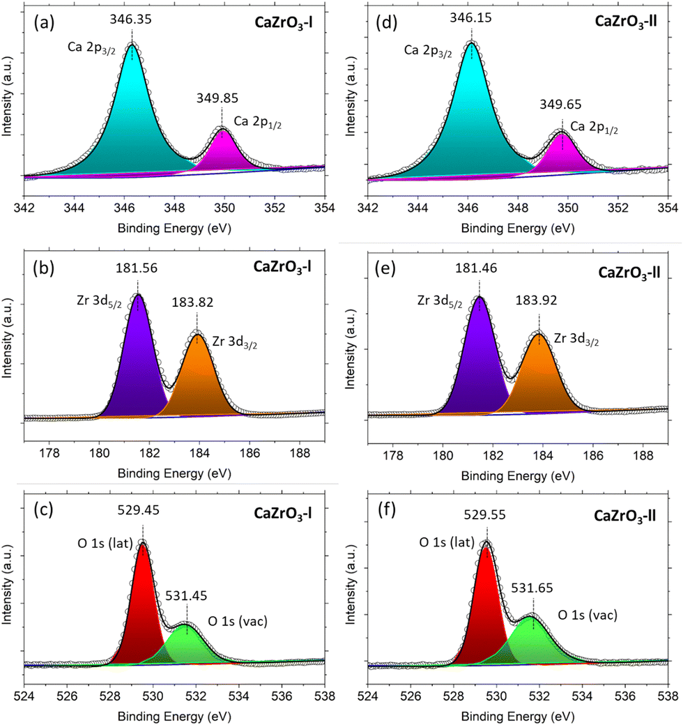 | ||
| Fig. 5 XPS spectra of CaZrO3-I and CaZrO3-II: (a)Ca 2p-l, (b) Zr 3d-l, (c) O 1s-l, (d) Ca 2p-ll, (e) Zr 3d-ll, (f) O 1s-ll. | ||
| Sample name | Ca 2p | Ca 2p | Zr 3d2 | Zr 3d3/2 | O 1s (lattice) | O1s (vacancy) |
|---|---|---|---|---|---|---|
| CaZrO3-l | 346.35 | 349.85 | 181.56 | 183.92 | 529.45 | 531.45 |
| CaZrO3-II | 346.15 | 349.65 | 181.46 | 183.82 | 529.55 | 531.65 |
| Standard values60,64 | 346–347 | 348–350 | 181–182 | 183–185 | 529–530 | 531–532 |
DFT calculations of defect formation in CaZrO3
The formation of CaZrO3 in the reaction CaO + ZrO2 → CaZrO3 instead of separated CaO and ZrO2 is associated with an energy gain of 0.06 eV per atom calculated on the basis of the total energies of reactants and products. Such a small difference in energy explains why all three components are formed during synthesis.Next, the formation of a single atomic vacancy in a bulk CaZrO3 crystal was considered. This is energetically unfavourable by 6.8 eV, 3.4 eV, and 5.9 eV, respectively, for the missing O, Ca, and Zr atom in the Ca4Zr4O12 supercell and by 8.0 eV, 3.9 eV, and 6.5 eV in the Ca32Zr32O96 supercell. This indicates that the formation of atomic vacancy defects is more favourable with higher densities of such defects, which was further confirmed by the calculations of two missing O atoms at different positions in the Ca32Zr32O96 supercell, showing that defect formation energy decreases to 7.0–7.5 eV per the missing O atom. It can also be seen that Ca defects can be formed more easily than Zr defects due to the number of their valence electrons; the missing Ca atom with two valence electrons causes less change in its vicinity compared to the Zr atom with four valence electrons.
Both the excess of Ca and Zr atoms in interstitial positions and the replacement of O atoms were also taken into account. Both scenarios, however, are energetically very unfavourable (Table S2, ESI†).
In addition, multiple defects in the crystal represented by the Ca12Zr12O36 supercell were created focusing on four stoichiometries, Ca12Zr11O28, Ca12Zr10O28, Ca12Zr12O28, and Ca11Zr12O26 with the latter two corresponding to experimental samples CaZrO3-I and CaZrO3-II. The two most important structures are shown in Fig. 6, all considered structures are shown in Section S3 (ESI†). Their relative energies to the structural ground state (GS) in systems of the same stoichiometry are in the range 0.5 2.9 eV. They are less than the defect formation energy of a single O vacancy and given the bottom-up approach used in the synthesis, many of these defects are likely to develop considering that this is a stochastic process. Moreover, bulk defects are preferred to a series of single defects in the crystal, which has a significant impact on the ionic conductivity of this material (vide infra), and the least stable defects contain significantly undercoordinated metal atoms.
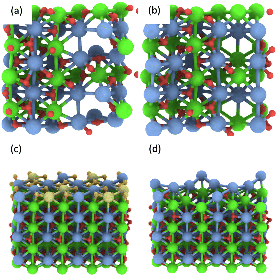 | ||
| Fig. 6 The most energetically favourable structure of the CaZrO3 bulk crystal from DFT calculations corresponding to the stoichiometry Ca12Zr10O28 (a) and Ca11Zr12O26 (CaZrO3-II) (b). (001) surface of CaZrO3 corresponding to the stoichiometry Ca32Zr32O96 (c). The yellow and orange spheres representing the Ca and O atoms were removed, creating a Ca29Zr32O69 slab corresponding to the stoichiometry of the CaZrO3-II sample (d). See Fig. 2 for the colour code. | ||
Finally, the formation of multiple vacancies at the (001) surface of CaZrO3 (Fig. 6 and Section S3, ESI†) was investigated. Two stoichiometries of Ca32Zr32O75 and Ca29Zr32O69 were considered, corresponding to the experimental systems CaZrO3-I and CaZrO3-II, respectively. Although the (110) surface may also be present in experimental samples (Table S4, ESI†), the focus was on the former surface because the atomic vacancies present there have a similar formation energy as in the bulk crystal (Table S5, ESI†), and thus the latter surface may be similar. The most energetically favourable defects create a crater-like structure at the (001) surface, while a long narrow channel through the whole slab is less favourable (Table S5, ESI†). Their role in ion conductivity is discussed below.
Thermal analysis of natural Limestone waste
Thermal analysis of the natural Limestone waste (Fig. 7) was performed to identify the exact temperatures at which the calcination and carbonation reactions take place. This information is crucial for determining the correct parameters that need to be applied for the cycling experiments. A 20% weight loss was observed between 350 °C to 590 °C which may be due to the decomposition of impurities present in the Limestone waste, since it was measured as received from the quarry with no further treatment (Fig. 7(a)). The second weight loss, from 80% down to 45%, between 610 °C and 910 °C is linked to the decomposition of Limestone to CO2 and CaO (Fig. 7(a)). This decomposition reaction is also known as calcination reaction, with a peak maximum observed at 785 °C (Fig. 7(b)). The Limestone sample was then kept isothermal at 1000 °C under a 90% CO2 atmosphere for 20 minutes, and then cooled down to room temperature. No weight gain was observed during the isothermal period, indicating that the temperature was too high for the carbonation reaction to take place. While cooling under a 90% CO2 atmosphere, a weight gain from 45% to 60% was observed due the absorption of CO2 into CaO to form CaCO3 (Fig. 7(a)). This reaction is also known as carbonation reaction, with an observed on-set temperature at 810 °C, a peak maximum at 884 °C and a completion at 900 °C (Fig. 7(b)). The weight gain for this reaction was only equal to 15 wt%, indicating that the carbonation reaction is incomplete (Fig. 7(a)).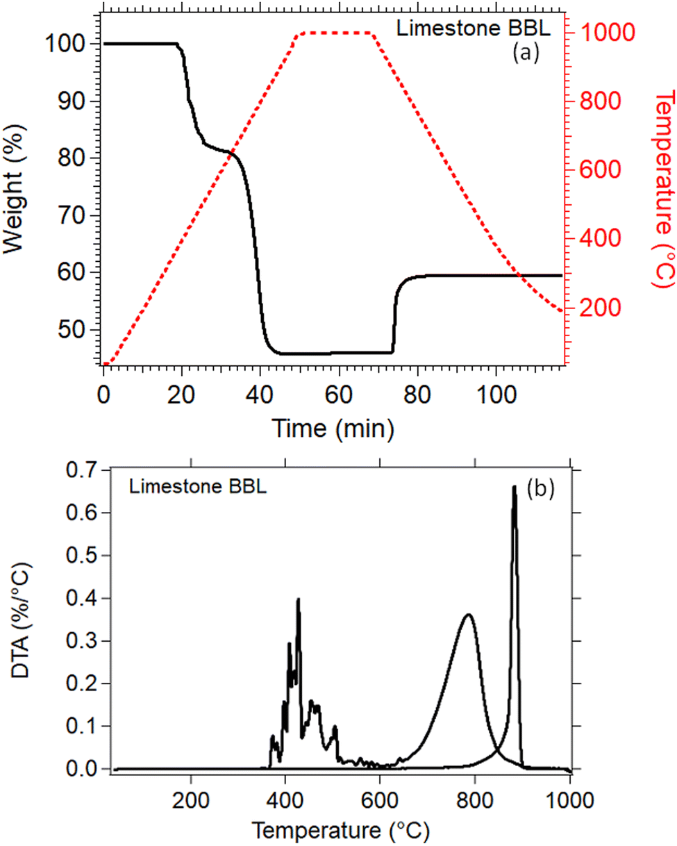 | ||
| Fig. 7 (a) TGA of Lim BBL in N2 environment up to 1000 °C (b) DTA of Lim BBL in N2 environment up to 1000 °C. | ||
Thermochemical (calcination/carbonation) cycling and heat storage performance for all samples
For the thermochemical cycling, a constant temperature was chosen at 884 °C corresponding to the peak temperature of the carbonation reaction (Fig. 7(b)). The reason for not choosing two different temperatures for the calcination and carbonation step for the cycling experiment, was mainly to simplify the system. It is well known in the literature that the calcination reaction is faster in comparison to the carbonation reaction.29,65–67 For this reason, 10 minutes were chosen for the calcination step and 20 minutes for the carbonation step during cycling. In total, 40 cycles were applied on all samples. Their effective conversion and heat storage densities were calculated and presented in Fig. 8 and Table 5. During the first ten cycles, the effective conversions dropped for all seven samples, indicating that the carbonation reaction is incomplete at the end of each cycle. This can easily be observed in Fig. S1 (ESI†) where the comparison of the reaction kinetics for all seven samples is plotted, showing a complete reaction for the calcination reaction and an incomplete carbonation reaction. It is reported in the literature that the carbonation process takes place in two stages.63 In the first stage, CO2 diffuses at a high rate into the first layers of the CaO grains, and forms a CaCO3 layer. This first stage is completed as soon as this CaCO3 layer is formed around the CaO grains. In the second stage, the carbonation reaction is restricted by a solid-state diffusion of Ca2+, O2− and CO32− ions across the formed CaCO3 layer, which significantly reduces the rate of the reaction. The purpose of using nanoadditives with high ionic conductivity like CaZrO3 is to reduce these kinetic barriers by facilitating the ionic mobility necessary for the carbonation reaction to complete. After the first ten cycles, a relatively stable cyclic performance was observed for all samples. Samples Lim BBL and 5R1 had the lowest effective conversion value of ∼0.44 and a heat storage density of 1651.4 kJ kg−1 and 1671.1 kJ kg−1. It is worth noticing that even though the same amount of nanoadditives (5 wt% CaZrO3) was used in sample 5R0.9, their effective conversion and heat storage density at the end of the 40th cycle was 0.50 and 1878.8 kJ kg−1, indicating that the difference of ionic conductivity within the samples plays a significant role in the cycling performance. The same can be observed for the best performing samples, 20R1 and 20R0.9, where the amount of nanoadditives used is exactly the same (20 wt%) but their performance is significantly different. In detail, after 40 cycles sample 20R1 has effective conversion value equal to 0.61 and a heat storage density of 2311.2 kJ kg−1. Whereas sample 20R0.9 has an effective conversion value equal to 0.70 and a heat storage density of 2640.3 kJ kg−1.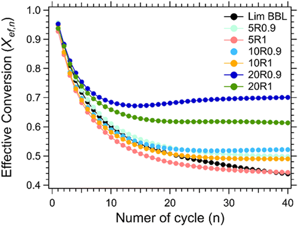 | ||
| Fig. 8 Effective conversion vs number of cycle for Lim BBL with different percentages of CaZrO3-I and CaZrO3-II. | ||
| # of cycles | Lim BBL | 5R1 | 5R0.9 | 10R1 | 10R0.9 | 20R1 | 20R0.9 |
|---|---|---|---|---|---|---|---|
| 10 | 2257.9 | 2124.5 | 2300.2 | 2190.1 | 2223.7 | 2481.2 | 2577.7 |
| 20 | 1912.2 | 1802.2 | 1992.6 | 1910.8 | 1978.6 | 2328.7 | 2565.8 |
| 30 | 1758.9 | 1705.0 | 1905.6 | 1851.2 | 1952.1 | 2327.0 | 2622.0 |
| 40 | 1651.4 | 1671.1 | 1878.8 | 1845.4 | 1966.0 | 2311.2 | 2640.3 |
Ionic conductivity from a DFT perspective
Theoretical DFT calculations were carried out for a better understanding of the ionic conductivity mechanism in CaZrO3. A series of static total energy calculations for a defective CaZrO3 with two a single missing O or Ca atoms, sampling migration paths for a single O or Ca between the two vacancies (Section S4, ESI†), revealed high migration barriers for both O (lowest barrier was 5.5 eV) and Ca (barrier at least 9.7 eV), Fig. 9.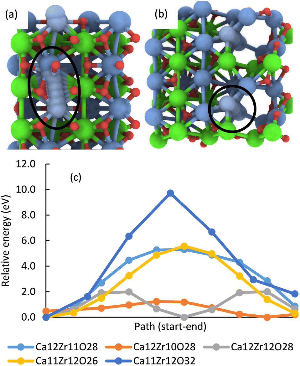 | ||
| Fig. 9 The most energetically favourable migration path enclosed by the black line for a single Ca through a defective CaZrO3 crystal with the stoichiometry Ca11Zr12O32 (dark blue line in (c)) (a) and Ca12Zr10O28 (orange line in (c)) (b). Energy profile of migration paths of a single Ca in systems with a given element composition (c). The energy is relative to the lowest point on the system's profile. Migration is easier with increasing channel width (cf. the text) and even a very narrow channel reduces the barrier by almost half (Ca12Zr11O28, Ca11Zr12O26, cf. Fig. S8–S11 in the ESI†). | ||
In multi-defect systems that correspond to the experimental stoichiometry, the migration of atoms for the GS geometry through the entire supercell (from one boundary to the opposite), i.e., through an endless channel (Section S5, ESI†) was investigated. In most of the studied systems, the lowest O migration barrier was reduced to 1.–1.9 eV, for Ca it was in the range 1.2–5.6 eV (Fig. 9), and for Zr the barriers for the two considered paths were 3.5 eV and 5.4 eV.
It should be noted that the above calculations did not consider possible structural changes related to ion transport. However, it still gives us a picture of the potential acting on the fast-moving ion in the CaZrO3 system.
The reliability of this approach was examined against a commonly used technique for finding reaction paths, i.e., the nudged elastic band (NEB) method.68,69 As the input path for the NEB calculations of Ca migration, a significantly energetically unfavourable path used for the static calculations was chosen. During the NEB calculations, this path was corrected to the more energetically favourable Ca migration path, which was also found earlier by static calculations. Thus, it can be expected that even in static calculations, energy-favourable paths are described quite precisely, while paths with high energy barriers will be corrected in the NEB method.
Note also that the paths associated with low diffusion barriers are those farther from the wall of the migration channel, because the elemental composition of the wall determines the potential acting on the migrating atom.
Finally, the desorption of O into the vacuum requires significant energy, at least 6.7 eV, which is comparable to the defect formation energy of a single O vacancy, i.e., 6.8 eV. Interestingly, in the presence of uncoordinated Ca atoms on the CaZrO3 surface, the first local maximum associated with O desorption is only 1.0 eV (Fig. S12, ESI†).
The desorption of the Ca atom from the surface was also investigated (Fig. S12, ESI†), and the energy required for this process (2.2–2.8 eV) is less than the defect formation energy of a single Ca vacancy (3.4 eV).
Composition of Limestone waste and CaZrO3/Limestone mixture samples
The composition of all samples before and after cycling is presented in Fig. 10. It is noticeable that the dominant crystal phase in all as-prepared samples (Fig. 10(a) and (c)) is CaCO3, including the Limestone waste, indicating that any impurities present are in very low concentration and not detectible by X-ray diffraction. The diffraction peaks assigned to the secondary CaZrO3 phase for the mixture samples become more obvious as the CaZrO3 content increases, as expected. After 40 cycles (Fig. 10(b) and (d)) the dominant phase in all samples is CaO along with CaCO3 and CaZrO3. No reaction products between CaCO3 and CaZrO3 upon cycling were observed, also confirmed by the in situ X-ray diffraction data presented in Fig. 11. Indicating, that CaZrO3 is chemically stable upon cycling.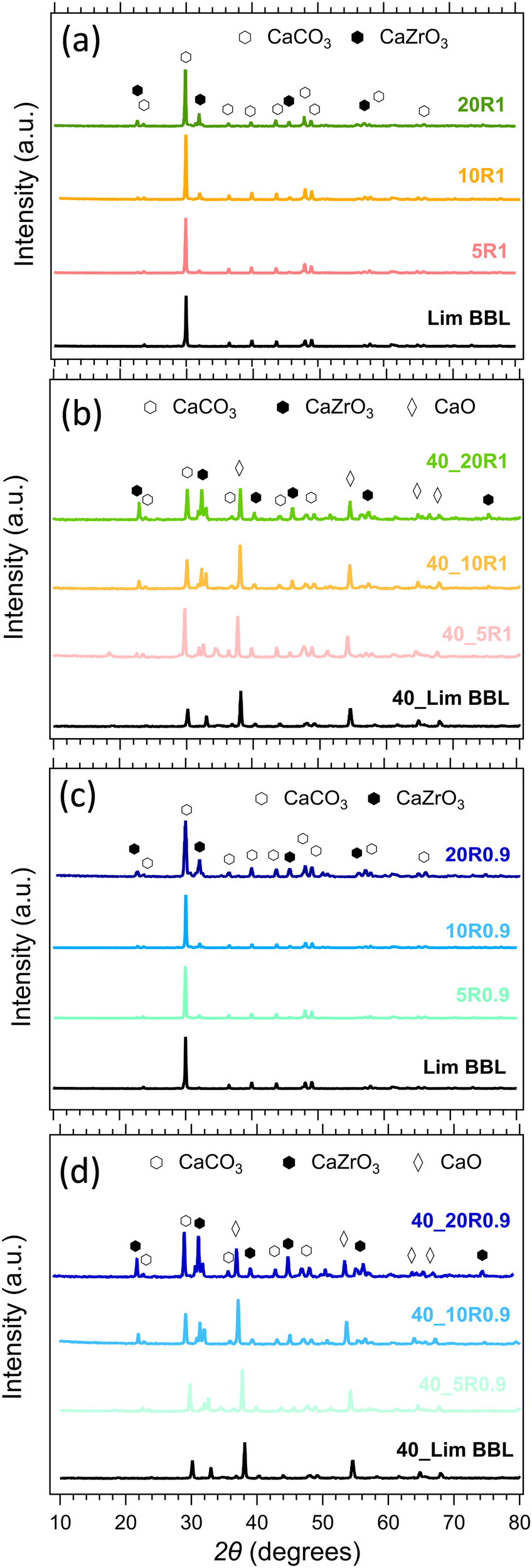 | ||
| Fig. 10 Powder X-ray diffraction patterns of the LimBBL (Limestone waste) sample and CaZrO3/CaCO3 mixture samples (a), (c) before and (b), (d) after 40 consecutive cycles. | ||
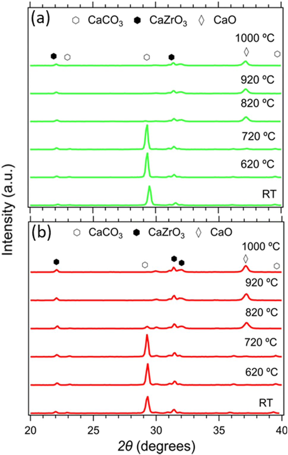 | ||
| Fig. 11 In situ X-ray diffraction data of the 20R1 and 20R0.9 samples from room temperature to 1000 °C. | ||
Morphology and physisorption analysis of Limestone waste and CaZrO3/CaCO3 mixture samples
EDS mapping and BET specific surface area analysis were carried out on all samples both before and after cycling to evaluate the morphological changes that take place upon cycling (Fig. 12, Fig. S2, S3, ESI† and Table 6). In Fig. 12 the SEM micrographs of the Lim BBL, 20R1 and 20R0.9 samples are presented, both before and after their 40 calcination/carbonation cycles. It can be observed that all three samples after cycling exhibit particles smaller in size in comparison to the ones before cycling, as reflected also in their calculated BET surfaces areas (Table 6), with the 40_10R1 and 40_10R0.9 samples having the highest BET surface areas. This may be due to some physical re-distribution of the Limestone grains and the CaZrO3 nanoadditves upon cycling; as noticed in Fig. 12 (after 40 cycles) where the CaZrO3 nanoparticles seem to be better distributed throughout the sample after cycling. These observations are also reflected for the other mixture samples as seen in Fig. S2 and S3 (ESI†). The very low specific surface area of all as-prepared samples (Table 6) is due to the fact that these samples were not ball milled and were used as-supplied. The average particle size of the Limestone waste was 2.28 μm as calculated from its associated SEM image (Fig. S4, ESI†).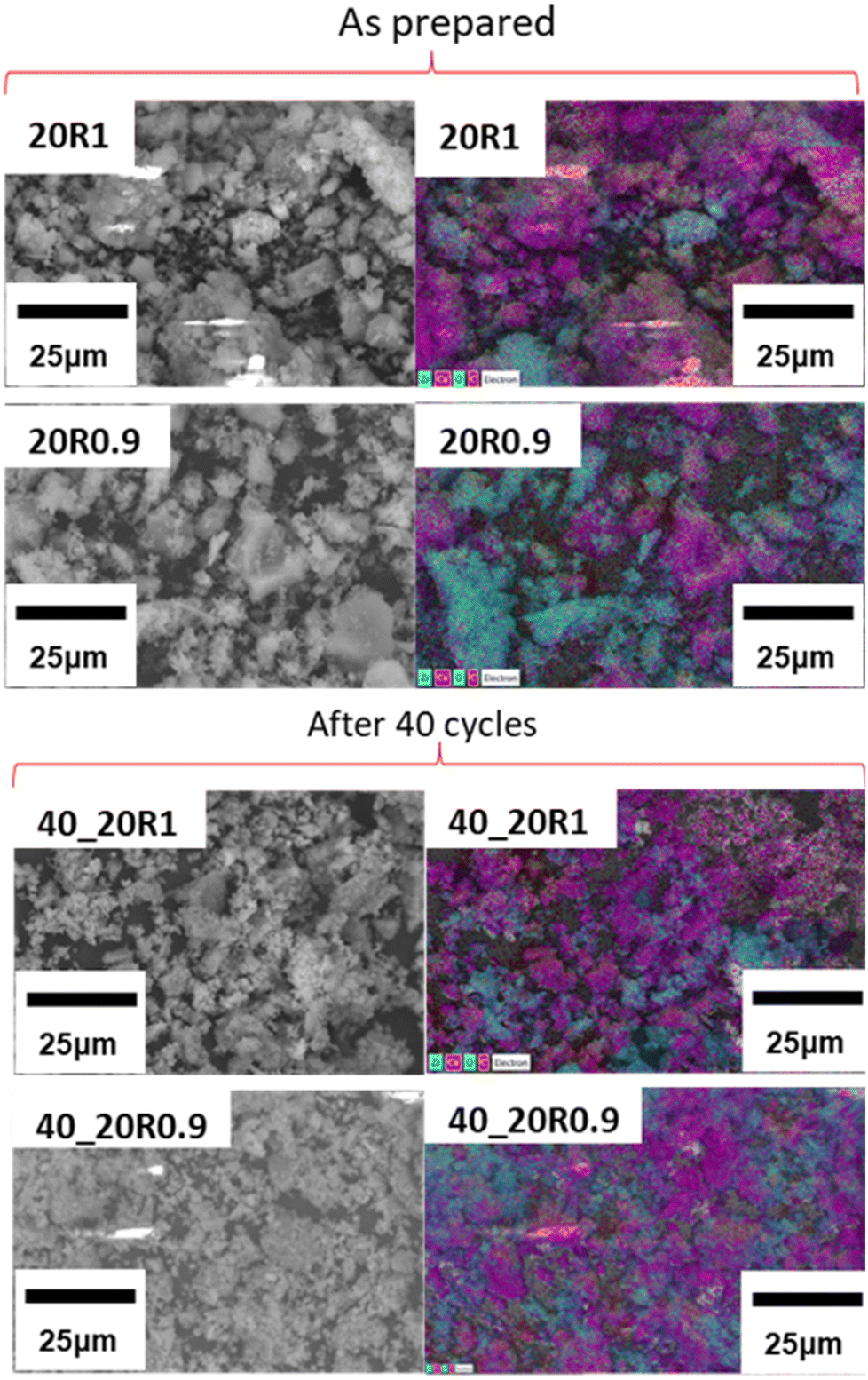 | ||
| Fig. 12 EDS mapping of 20% CaZrO3 samples, before and after 40 cycles. Blue is for Zr, purple is for Ca, green is for O and red is for C. | ||
| Sample ID | Before cycling | After cycling |
|---|---|---|
| Lim BBL | 1.03 ± 0.1 | 4.53 ± 0.5 |
| 5R1 | 1.15 ± 0.1 | 3.77 ± 0.4 |
| 10R1 | 2.20 ± 0.2 | 4.81 ± 0.5 |
| 20R1 | 2.70 ± 0.3 | 3.29 ± 0.3 |
| 5R0.9 | 2.09 ± 0.2 | 1.56 ± 0.2 |
| 10R0.9 | 1.91 ± 0.2 | 5.10 ± 0.5 |
| 20R0.9 | 2.10 ± 0.2 | 3.89 ± 0.4 |
Conclusions
The cycling performance of Limestone was improved by designing CaZrO3 nanoadditive. CaZrO3 samples with two different Ca:Zr ratio was successfully synthesized by wet precipitation method. XRD analysis confirm the synthesis of CaZrO3. CaZrO3 nanoparticles were observed in SEM and TEM images. XPS analysis revealed that, the percentage of Ovac of the CaZrO3-I and CaZrO3-II samples were 23.43% and 28.58% respectively. Structures corresponding to the experimental stoichiometry were investigated by DFT calculations. They revealed that multiple defects are formed in CaZrO3, and their presence improves the ionic conductivity of this material. Out of all mixture samples the one with 20% CaZrO3-II exhibited the best performance with an effective conversion of 0.7 and energy density of 2640 kJ kg−1. The second best performing mixture sample was the one with 20% CaZrO3-I; exhibiting an effective conversion of 0.61 and energy density of 2311 kJ kg−1. The XRD analysis of all samples after cycling confirmed that CaZrO3 did not react with Limestone. The SEM/EDS analysis of the samples after cycling showed a better distribution of Limestone and CaZrO3 particles; which can be responsible for stable cycling performance.
Conflicts of interest
There are no conflicts to declare.Acknowledgements
MVS acknowledges the financial support from the UCD Ad Astra Fellowship Programme and the Technology Transfer Strengthening Initiative Programme from Enterprise Ireland (reference grant number 68001). RA acknowledges the financial support from the UCD Ad Astra Studentship Programme. All authors would like to thank Prof. James Sullivan and Kristy Stanley for providing access to the TA Q500 Thermogravimetric analyser located at the UCD School of Chemistry. The work in Olomouc was supported by the Operational Programme for Research, Development and Education of the European Regional Development Fund (Project no. CZ.02.1.01/0.0/0.0/16_019/0000754 of the Ministry of Education, Youth and Sports of the Czech Republic). JN acknowledges support by Palacký University Olomouc (project IGA_PrF_2022_019). The IT4Innovations National Supercomputing Center is gratefully acknowledged for providing generous computational resources supported by the Ministry of Education, Youth and Sports of the Czech Republic through the e-INFRA CZ (No. 90140). All authors would like to thank Bennettsbridge Limestone Quarries, Ireland for providing Limestone waste for this study.References
- I. Irena, Report, International Renewable Energy Agency, Abu Dhabi, 2018 Search PubMed.
- Z. Yuan, L. Liang, Q. Dai, T. Li, Q. Song, H. Zhang, G. Hou and X. Li, Joule, 2022, 6, 884–905 CrossRef CAS.
- J. Haas, L. Prieto-Miranda, N. Ghorbani and C. Breyer, Renewable Energy, 2022, 181, 182–193 CrossRef.
- Y. Yang, Y. Li, X. Yan, J. Zhao and C. Zhang, Energies, 2021, 14, 6847 CrossRef CAS.
- R. Paul, M. Wang and A. Roy, ACS Appl. Nano Mater., 2020, 3, 10418–10426 CrossRef CAS.
- U. Pelay, L. Luo, Y. Fan, D. Stitou and M. Rood, Renewable Sustainable Energy Rev., 2017, 79, 82–100 CrossRef.
- J. Cot-Gores, A. Castell and L. F. Cabeza, Renewable Sustainable Energy Rev., 2012, 16, 5207–5224 CrossRef.
- A. I. Fernandez, M. Martínez, M. Segarra, I. Martorell and L. F. Cabeza, Sol. Energy Mater. Sol. Cells, 2010, 94, 1723–1729 CrossRef CAS.
- C. Wani and P. Kumar Loharkar, Mater. Today: Proc., 2017, 4, 10264–10267 Search PubMed.
- A. Carro, R. Chacartegui, C. Ortiz and J. Becerra, Energy, 2022, 125064 CrossRef CAS.
- P. Pardo, A. Deydier, Z. Anxionnaz-Minvielle, S. Rougé, M. Cabassud and P. Cognet, Renewable Sustainable Energy Rev., 2014, 32, 591–610 CrossRef CAS.
- K. Wang, T. Yan, R. Li and W. Pan, J. Energy Storage, 2022, 50, 104612 CrossRef.
- N. R. Rhodes, A. Barde, K. Randhir, L. Li, D. W. Hahn, R. Mei, J. F. Klausner and N. AuYeung, ChemSusChem, 2015, 8, 3793–3798 CrossRef CAS PubMed.
- Q. Zhao, J. Lin, H. Huang, Z. Xie and Y. Xiao, J. Energy Storage, 2022, 50, 104259 CrossRef.
- R. Han, S. Xing, X. Wu, C. Pang, S. Lu, Y. Su, Q. Liu, C. Song and J. Gao, Renewable Energy, 2022, 181, 267–277 CrossRef CAS.
- N. Amghar, C. Ortiz, A. Perejón, J. M. Valverde, L. P. Maqueda and P. E. S. Jiménez, Sol. Energy Mater. Sol. Cells, 2022, 238, 111632 CrossRef CAS.
- X. Qu, Y. Li, P. Li, Q. Wan and F. Zhai, Front. Mater. Sci., 2015, 9, 317–331 CrossRef.
- M. Hirscher, V. A. Yartys, M. Baricco, J. Bellosta von Colbe, D. Blanchard, R. C. Bowman, D. P. Broom, C. E. Buckley, F. Chang, P. Chen, Y. W. Cho, J.-C. Crivello, F. Cuevas, W. I. F. David, P. E. de Jongh, R. V. Denys, M. Dornheim, M. Felderhoff, Y. Filinchuk, G. E. Froudakis, D. M. Grant, E. M. Gray, B. C. Hauback, T. He, T. D. Humphries, T. R. Jensen, S. Kim, Y. Kojima, M. Latroche, H.-W. Li, M. V. Lototskyy, J. W. Makepeace, K. T. Møller, L. Naheed, P. Ngene, D. Noréus, M. M. Nygård, S.-I. Orimo, M. Paskevicius, L. Pasquini, D. B. Ravnsbæk, M. Veronica Sofianos, T. J. Udovic, T. Vegge, G. S. Walker, C. J. Webb, C. Weidenthaler and C. Zlotea, J. Alloys Compd., 2020, 827, 153548 CrossRef CAS.
- P. Larpruenrudee, N. S. Bennett, Y. Gu, R. Fitch and M. S. Islam, Sci. Rep., 2022, 12, 1–16 CrossRef PubMed.
- C. Comanescu, Int. J. Mol. Sci., 2022, 23, 7111 CrossRef CAS PubMed.
- M. Schmidt and M. Linder, Appl. Energy, 2017, 203, 594–607 CrossRef CAS.
- K. T. Møller, T. D. Humphries, A. Berger, M. Paskevicius and C. E. Buckley, Chem. Eng. J. Adv., 2021, 8, 100168 CrossRef.
- K. E. N’Tsoukpoe, H. Liu, N. Le Pierrès and L. Luo, Renewable Sustainable Energy Rev., 2009, 13, 2385–2396 CrossRef.
- A. Martínez, Y. Lara, P. Lisbona and L. M. Romeo, Int. J. Greenhouse Gas Control, 2012, 7, 74–81 CrossRef.
- A. Bayon, R. Bader, M. Jafarian, L. Fedunik-Hofman, Y. Sun, J. Hinkley, S. Miller and W. Lipiński, Energy, 2018, 149, 473–484 CrossRef CAS.
- C. Prieto, P. Cooper, A. I. Fernández and L. F. Cabeza, Renewable Sustainable Energy Rev., 2016, 60, 909–929 CrossRef CAS.
- K. T. Møller, A. Berger, M. Paskevicius and C. E. Buckley, J. Alloys Compd., 2022, 891, 161954 CrossRef.
- Y. Zhou, Z. Zhou, L. Liu, X. She, R. Xu, J. Sun and M. Xu, Energy Fuels, 2021, 35, 18778–18788 CrossRef CAS.
- K. T. Møller, A. Ibrahim, C. E. Buckley and M. Paskevicius, J. Mater. Chem. A, 2020, 8, 9646–9653 RSC.
- Z. Sun, S. Luo, P. Qi and L.-S. Fan, Chem. Eng. Sci., 2012, 81, 164–168 CrossRef CAS.
- C. Li, Y. Li, C. Zhang, Y. Dou, Z. He and J. Zhao, Fuel Process. Technol., 2022, 237, 107444 CrossRef CAS.
- X. Tian, S. Lin, J. Yan and C. Zhao, Chem. Eng. J., 2022, 428, 131229 CrossRef CAS.
- A. Mathew, N. Nadim, T. T. Chandratilleke, M. Paskevicius, T. D. Humphries and C. E. Buckley, Sol. Energy, 2022, 241, 262–274 CrossRef CAS.
- H. Sun, Y. Li, X. Yan, J. Zhao and Z. Wang, Appl. Energy, 2020, 263, 114650 CrossRef CAS.
- A. A. Khosa, T. Xu, B. Xia, J. Yan and C. Zhao, Sol. Energy, 2019, 193, 618–636 CrossRef CAS.
- T. Richardson, R. K. Vijayaraghavan, P. McNally and M. V. Sofianos, Available at SSRN 4156637.
- A. A. Khosa and C. Zhao, Sol. Energy, 2019, 188, 619–630 CrossRef CAS.
- X. Chen, X. Jin, Z. Liu, X. Ling and Y. Wang, Energy, 2018, 155, 128–138 CrossRef CAS.
- J. M. Valverde, M. Barea-López, A. Perejón, P. E. Sánchez-Jiménez and L. A. Pérez-Maqueda, Energy Fuels, 2017, 31, 4226–4236 CrossRef CAS.
- B. Sarrión, A. Perejón, P. E. Sánchez-Jiménez, L. A. Pérez-Maqueda and J. M. Valverde, J. CO2 Util., 2018, 28, 374–384 CrossRef.
- B. Sarrion, P. E. Sanchez-Jimenez, A. Perejon, L. A. Perez-Maqueda and J. M. Valverde, ACS Sustainable Chem. Eng., 2018, 6, 7849–7858 CrossRef CAS.
- S. M. Alay-e-Abbas, S. Nazir, S. Cottenier and A. Shaukat, Sci. Rep., 2017, 7, 8439 CrossRef PubMed.
- P. Han, H. Lv, X. Li, S. Wang, Z. Wu, X. Li, Z. Mu, X. Li, C. Sun, H. Wei and L. Ma, Catal. Sci. Technol., 2021, 11, 3697–3705 RSC.
- M. Zhao, M. Bilton, A. P. Brown, A. M. Cunliffe, E. Dvininov, V. Dupont, T. P. Comyn and S. J. Milne, Energy Fuels, 2014, 28, 1275–1283 CrossRef CAS.
- M. Pollet, S. Marinel and G. Desgardin, J. Eur. Ceram. Soc., 2004, 24, 119–127 CrossRef CAS.
- C. S. Prasanth, H. Padma Kumar, R. Pazhani, S. Solomon and J. K. Thomas, J. Alloys Compd., 2008, 464, 306–309 CrossRef CAS.
- G. Kresse and J. Furthmüller, Comput. Mater. Sci., 1996, 6, 15–50 CrossRef CAS.
- G. Kresse and J. Hafner, Phys. Rev. B: Condens. Matter Mater. Phys., 1993, 47, 558–561 CrossRef CAS PubMed.
- G. Kresse and J. Furthmüller, Phys. Rev. B: Condens. Matter Mater. Phys., 1996, 54, 11169–11186 CrossRef CAS PubMed.
- G. Kresse and J. Hafner, Phys. Rev. B: Condens. Matter Mater. Phys., 1994, 49, 14251–14269 CrossRef CAS PubMed.
- G. Kresse and D. Joubert, Phys. Rev. B: Condens. Matter Mater. Phys., 1999, 59, 1758–1775 CrossRef CAS.
- P. E. Blöchl, Phys. Rev. B: Condens. Matter Mater. Phys., 1994, 50, 17953–17979 CrossRef PubMed.
- J. P. Perdew, K. Burke and M. Ernzerhof, Phys. Rev. Lett., 1996, 77, 3865–3868 CrossRef CAS PubMed.
- J. P. Perdew, K. Burke and M. Ernzerhof, Phys. Rev. Lett., 1997, 78, 1396 CrossRef CAS.
- S. Grimme, J. Antony, S. Ehrlich and H. Krieg, J. Chem. Phys., 2010, 132, 154104 CrossRef PubMed.
- K. Momma and F. Izumi, J. Appl. Crystallogr., 2011, 44, 1272–1276 CrossRef CAS.
- https://github.com/wwwtyro/speck (accessed 14/02/2022).
- P. Han, X. Li, C. Jin, X. Tan, W. Sun, S. Wang, F. Ding, X. Li, H. Jin and C. Sun, Chem. Eng. J., 2022, 429, 132218 CrossRef CAS.
- R. S. André, S. M. Zanetti, J. A. Varela and E. Longo, Ceram. Int., 2014, 40, 16627–16634 CrossRef.
- R. Koirala, K. R. Gunugunuri, S. E. Pratsinis and P. G. Smirniotis, J. Phys. Chem. C, 2011, 115, 24804–24812 CrossRef CAS.
- M. López Granados, A. Gurbani, R. Mariscal and J. L. G. Fierro, J. Catal., 2008, 256, 172–182 CrossRef.
- B. Luo, H. Dong, D. Wang and K. Jin, J. Am. Ceram. Soc., 2018, 101, 3460–3467 CrossRef CAS.
- B. Luo, J. Appl. Phys., 2017, 122, 195104 CrossRef.
- G. Cabello, L. Lillo, C. Caro, G. E. Buono-Core, B. Chornik, M. Flores, C. Carrasco and C. A. Rodriguez, Ceram. Int., 2014, 40, 7761–7768 CrossRef CAS.
- A. M. López-Periago, J. Fraile, P. López-Aranguren, L. F. Vega and C. Domingo, Chem. Eng. J., 2013, 226, 357–366 CrossRef.
- Y. A. Criado, B. Arias and J. C. Abanades, Ind. Eng. Chem. Res., 2018, 57, 12595–12599 CrossRef CAS.
- B. R. Stanmore and P. Gilot, Fuel Process. Technol., 2005, 86, 1707–1743 CrossRef CAS.
- G. Mills and H. Jónsson, Phys. Rev. Lett., 1994, 72, 1124–1127 CrossRef CAS PubMed.
- G. Mills, H. Jónsson and G. K. Schenter, Surf. Sci., 1995, 324, 305–337 CrossRef CAS.
Footnote |
| † Electronic supplementary information (ESI) available: CO2 uptake/release capacity data, EDS mapping, SEM micrograph, computational details, DFT results. See DOI: https://doi.org/10.1039/d2ma01083f |
| This journal is © The Royal Society of Chemistry 2023 |