Holographic flow scanning cytometry overcomes depth of focus limits and smartly adapts to microfluidic speed

Abstract

Space-time digital holography (STDH) maps holograms in a hybrid space-time domain to achieve extended field of view, resolution enhanced, quantitative phase-contrast microscopy and velocimetry of flowing objects in a label-free modality. In STDH, area sensors can be replaced by compact and faster linear sensor arrays to augment the imaging throughput and to compress data from a microfluidic video sequence into one single hybrid hologram. However, in order to ensure proper imaging, the velocity of the objects in microfluidic channels has to be well-matched to the acquisition frame rate, which is the major constraint of the method. Also, imaging all the flowing samples in focus at the same time, while avoiding hydrodynamic focusing devices, is a highly desirable goal. Here we demonstrate a novel processing pipeline that addresses non-ideal flow conditions and is capable of returning the correct and extended focus phase contrast mapping of an entire microfluidic experiment in a single image. We apply this novel processing strategy to recover phase imaging of flowing HeLa cells in a lab-on-a-chip platform even when severely undersampled due to too fast flow while ensuring that all cells are in focus.

---

Introduction

Optofluidic microscopy is a well-established paradigm where precise control of microfluidic streams is smartly exploited to enhance imaging of biological samples at the single cell level and to allow new accurate assay protocols.^1,2 Label-free imaging approaches are often preferable, being non-invasive and not dependent on reagents, dyes and markers. Imaging flow-cytometry, automated cell sorting, counting and classification, in flow tomography, study of cell mechanics and morphometry, analysis of cell to cell interaction and reaction to drugs are good examples in this sense.^1–6 In this framework, digital holography (DH) in transmission microscope configuration is one of the most suitable methods for high-throughput lab-on a chip microfluidic imaging.^7–13 DH gives access to the complex amplitude of the sample, i.e. both the intensity and the quantitative phase-contrast map are available after hologram post-processing, so that the object morphology and its optical thickness can be measured. Since the phase of the object wavefront is retrievable, a hologram can be back-propagated to adjust the focus of the sample. Thus, DH implicitly encodes in a 2D image the diffraction patterns from out of focus objects flowing in a 3D microfluidic volume. Numerical automatic refocusing based on contrast optimization 2D metrics allows retrieving each sample in its best-focus plane¹⁴ to get the final phase-contrast map. DH has been successfully applied to a large variety of microfluidic experiments for basic biology research and diagnostics, e.g. for single-cell analysis, 3D tracking and classification, blood disease detection through all optical discriminators, acoustic field measures, liquid biopsy, and drug resistance in cancer cells.^{6,8,10–13,15–18}

Collecting a statistically relevant amount of data from each patient is necessary to provide a reliable diagnostic response, and high-throughput volumetric DH imaging is suitable to meet such requirement. In order to solve the trade-off existing in microscopy between object magnification and field of view (FoV), scanning approaches have been proposed.^19–26 These create a synthetic enlarged FoV while keeping the desired object magnification. Lensless object scanning holography and synthetic aperture holography acquire multiple holograms while scanning the object or the 2D sensor to enlarge the FoV along the scanning axis and to counteract the effects of coherent noise.^22,24,26,27 However, proper hologram stitching has to be performed in the Fourier domain. This is a non-trivial and time-consuming procedure whose performance may severely depend on the object spectrum shape. In scanning-based imaging, the price to pay for the FoV extension is the need to mechanically scan the object. Hence, the more natural application for scanning approaches is microfluidics, where the object motion is an intrinsic feature of the system and can be used to achieve unlimited FoV. The optofluidic microscope (OFM) was the first breakthrough that fully exploited the accurate microfluidic flow control.¹⁹ The sample was allowed to flow along a device where skewed apertures provided optical access. Proper design of the inter-aperture spacing allowed increasing the resolution while taking advantage of the FoV extension. The main limit of OFM is the need to keep the sample in close contact with the apertures which prevents one from using it for high-throughput imaging onboard deep LoC devices. Light diffraction from a slit and a cylindrical collecting lens were coupled to achieve in-flow tomographic imaging.^7,21,28 A microlens array added to the illumination arm of an epifluorescence microscope was also used to obtain a multi-focal excitation pattern while the sample was allowed to flow along a microfluidic path.²⁹ Image deconvolution was demonstrated to provide optofluidic intensity microscopy beyond the resolution limit.²⁹ Lensless near-field imaging using three LEDs has been also introduced.²⁷ In this case, iterative phase retrieval algorithms are needed to reconstruct the object. In a recent work, ptychographic imaging has been adapted to operate in flow cytometry mode.³⁰ In order to avoid iterative phase retrieval and related convergence problems, off-axis or slightly off-axis DH configurations should be used. In addition, the combination of deep learning and holographic flow cytometry creates several new possibilities.^5,17 Nevertheless, cell imaging in microfluidic channels (MFC) based on deep learning usually requires a large amount of experimental data during the training process. As a general rule of thumb, a deep net cannot outperform the quality of the dataset it has been fed with. The proposed approach, adaptive imaging flow cytometry, can be realized without AI-training and is robust against unexpected situations that would require retraining deep nets. Space-time digital holography (STDH) and space-time scanning interferometry (STSI) replace the 2D sensors with a more compact and faster linear sensor array (LSA) to augment the throughput and promote miniaturization.^20,23,31,32 In both cases, the samples are mapped in a hybrid space-time domain, which corresponds to a projection of the modulated fringes. In the case of STSI, three lines of the LSA are sufficient to create synthetic interferograms shifted in phase of the desired offsets, and thus three-step phase shifting algorithms can be applied to directly recover the phase with custom FoV along the scanning axis, without using piezoelectric actuators.²⁰ A general problem with piezo transducer-based phase-shifting methods is a strong lack of temporal resolution. Moreover, accurate phase shifts have to be generated, while the appearance of nonlinear response induced by a piezoelectric transducer³³ can affect the measurements. Essentially, the main use condition of generalized phase-shifting interferometry (PSI) lies in static cell imaging,³⁴ a limitation that STDH can overcome to embed all the cases of moving objects. STSI has been also used with an LED source to image cells, blood smears and tissue slides.^32,35 In the case of STDH, conventional back-propagation methods are demonstrated to properly refocus the object and to retrieve its phase map with enlarged FoV when these are applied to the projected fringe pattern.^23,32,33 Thanks to the object motion, STDH has been recently demonstrated to enhance spatial resolution beyond the limits of the employed optical system by self-assembling the object spatial frequencies, acting just like a synthetic aperture radar. In the case of oblique STDH, resolution can be improved in two dimensions by a 1D scan.³⁶ Thus, STDH is a very promising method well suited for imaging cells onboard LoC devices, and has been recently coupled to hydrodynamic focusing and a high frame rate LSA to achieve high-throughput mapping of human colorectal-tumour cell lines.³³ However, in order to ensure undistorted STDH imaging, a proper matching has to be provided between the sample speed and the recording frame rate.^20,23,37 This may be hard to achieve in the case of non-perfect flow control of the LoC system and its microfluidic pump.^31,32 Besides, even in the case of ideal flow control,³⁸ the velocity distribution inside the channel makes the matching dependent on the sample position. Hence, some cells might be undersampled if they flow too fast, which results in a squeezed shape in the STDH,³¹ or oversampled and mapped as elongated if they flow too slowly.³² When the object shape is known, the shape factor and sample libraries can be used for particle image velocimetry and 3D tracking.³¹ However, imaging has never been recovered in these cases. On the other hand, in the case of long microfluidic experiments, it is desirable to get in focus in one single gigapixel DH reconstruction all the samples flowing inside the 3D channel volume.^39,40 This makes the related issues more difficult to handle, since the mismatch between sampling and cell velocities also depends on the propagation plane. Moreover, automatic refocusing based on 2D regions of interest can fail in the case of high-density samples.

In this paper, we show an improved spatio-temporal scanning strategy, hereafter called adaptive space-time digital holography (ASTDH). The proposed approach and related processing pipeline have been specifically conceived for managing STDH experiments in non-ideal flow conditions and thus for attaining correct quantitative phase-contrast maps despite the non-uniformities in the microflow. We introduce two correction parameters, P and α, during the hologram self-assembly and numerical reconstruction process. The P parameter acts on the assembling process of the space-time hologram, it allows compensating the main mismatch between the nominal speed and the actual speed established inside a channel, provided that the mismatch difference is an integer multiple of the pixel in the image plane. The α factor acts in the DH propagation kernel and allows mitigating the effects of undersampling due to residual subpixel mismatches. Actually, we noted that the aforementioned subpixel mismatch can be thought as a sort of anamorphic aberration in the scanning digital hologram.⁴¹ This analogy allowed us to find a systematic solution to the problem. We show how this factor depends on the propagation plane and the sample position along the time axis, and we propose a criterion to estimate its distribution. Moreover, by correcting the disturbances due to subpixel mismatches, an extended focus imaging (EFI) criterion^40,42,43 is applied to obtain also in sharp focus all the samples within the microfluidic volume corresponding to a long ASTDH experiment, independently on their position. We test the ASTDH processing pipeline by imaging, in amplitude and phase-contrast, HeLa cells flowing with a speed higher than the velocity imposed by the matching constraint. We demonstrate the correct recovering of the undersampled information and we show that a 1D automatic refocusing criterion applied to small STDH strips efficiently returns all the cells in best focus in the same extended FoV image, thus also saving computational time.

Working principle

To implement ASTDH imaging for cells in non-ideal flow, four essential processes need to be performed sequentially: a) space-time hologram assembly based on conventional STDH and P factor adjustment; b) efficient phase shifting of space–time holograms; c) depth of focus (DoF) extension; d) calculation of the α factor for subpixel calibration of cells in sharp focus.

Hybrid flow scanning holography for non-ideal flow

For a DH setup in off-axis microscopy configuration, let O and R be the object and the reference beams. Without losing generality, the reference beam can be assumed to be a plane wave tilted of an angle θ with respect to the object beam, thus producing a carrier in the recording plane with frequency ν = sin θ/λ, where λ indicates the wavelength of the light probe. The hologram in the acquisition plane, H(x, y), is the intensity of the coherent superposition between O and R:

H = |R + O|² = |R|² + |O|² + 2|R||O|cos[2πv(x + y) − ϕ], (1)

where we omitted for brevity the dependence on the spatial variables, ϕ is the phase of the object in the hologram plane (x, y) and we assumed for the sake of clarity that the fringes form a 45° angle with the x axis. In conventional off-axis DH, the object can be retrieved by demodulating eqn (1), and then refocused by wavefront back-propagation algorithms that solve numerically the diffraction integral. In conventional STDH, the object movement is exploited to create a synthetic hologram represented in a hybrid space-time domain, as shown in Fig. 1(a and b). Let P be the number of consecutive lines, normal to the cells' flow direction, used for sampling the hologram sequence and assembling the STDH. If one single line of the hologram, x₀, is sampled with frame rate F_r while the objects flow, i.e. P = 1, the STDH of the experiment can be obtained:

H(t, y) = [H(x₀, y; t₁), …, H(x₀, y; t_K)], (2)

where K is the total number of frames captured and defines the length of the STDH, i.e. its dimension along the time axis. In principle, K can assume an arbitrary value, and thus a STDH has unlimited FoV along the time axis. The STDH mapping corresponds to a projection of the interference fringes in the new hybrid domain, which is demonstrated to possess the refocusing capability of conventional DHs. Let H_d(t, y) be the STDH demodulated in the hybrid Fourier domain and let C_A(t′, y′; z) = P_z{H_d(t, y)} be the space-time complex amplitude reconstructed in the plane (t′, y′) at distance z from the hologram plane through the propagation operator P_z{…}. In the case the Fresnel method is used for propagation, we obtain

C_A(t′, y′; z) ∝ [scr F, script letter F]{H_d(t, y)e^{[iπ(y2+t2)/λz]}}, (3)

where [scr F, script letter F]{…} denotes the Fourier transform operator, implemented through a FFT2 algorithm. If the following matching condition between the object speed, v_x, and the frame rate is fulfilled

v_x = (Δx/M_z)F_r, (4)

then an undistorted image of the object is obtainable in its own image plane.^20,23,31 In eqn (4), M_z is the sample magnification in the image plane, which is in turn slightly dependent on the sample position inside the channel. Hence, even in ideal flow conditions, eqn (4) cannot be exactly respected for all the flowing samples unless accurate hydrodynamic focusing is provided. However, the speed itself often does not match the constraint, due to non-perfect flow control and/or the parabolic velocity distribution typical of microfluidic channels. Thus, the synthetic space-time hologram might show some objects severely undersampled and in turn squeezed,³¹ or elongated when they flow too slowly.³²Fig. 1(c) shows the conventional STDH obtained using the time interval from 28.40 s to 40.74 s of the recorded Hela cells' flow. The sampling line x₀ has been set as the center line (x₀ = 518), and P = 1. The modulated pattern of interference fringes was projected onto the hybrid space-time domain and reassembled by time series. As a result of undersampling, the Hela cells' images, indicated by red arrows, appear like squeezed to ellipse shapes in the synthetic representation. In order to overcome this issue in conventional STDH, one strategy could be replacing single line assembly with stripe assembly. In other words, a STDH can be created by defining a virtual pixel made of P consecutive sampling lines, where P > 1. This solution is in the middle between conventional DH (where P equals the sensor lateral dimension) and our first implementation of STDH (where P = 1). Herein, we define a virtual pixel, Δx_p = PΔx, P being a positive integer number. Thus, instead of selecting one single line of the sensor, we use P lines for each time frame to create the STDH. This step helps relaxing the matching constraint, i.e. replacing Δx with Δx_p reduces the difference between the first and second hand of eqn (4). Fig. 1(d) shows the STDH corresponding to the same time interval of Fig. 1(c) but obtained using P = 5. The enlarged details of one of the selected cells are shown in solid box areas for both cases. The shape of the selected cell is preliminary restored with the calibration factor P. As shown in the zoom areas of Fig. 1(c and d), once P is set to 5, the cell diameter D_{P = 5} is closer to the ground truth obtained from the conventional hologram than the squeezed diameter obtainable when P = 1. Therefore, STDH based on virtual pixel assembly is a feasible strategy to relax the problem of dealing with non-ideal cell flow-scanning imaging, since mismatches that are integer multiples of the pixel size in the image plane can be removed. Since in microfluidic experiments the flux is not always uniform in time and space, in principle the estimation of the optimal P factor should be repeated at least for groups of cells to ensure that undersampling does not occur. As it will be discussed in the following, in our case setting P = 5 ensures that 85% of the cells are well sampled. Further refinements allow recovering the remaining 15% of undersampled cells by estimating the P factor for groups of cells. An experimental validation and discussion about the role of the P factor is presented in the ESI.†

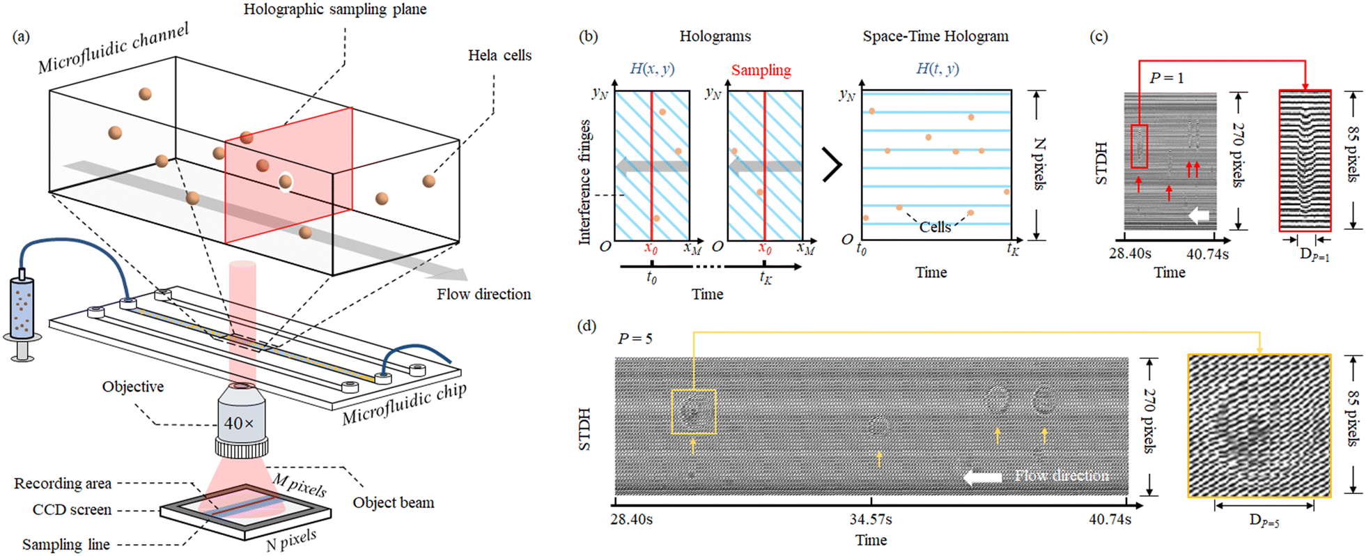Fig. 1 Working principle of conventional STDH. (a) Sketch of the LoC-based imaging system in object arm. The reference beam arm is not depicted here for the sake of clarity. (b) Synthesis of a conventional STDH from a sequence of digital holograms. (c) Corresponding conventional STDH mapping, where P is set to 1. (d) STDH assembled by virtual pixel, where P is set to 5. The coloured arrows in (c and d) show the cell locations. The enlarged details of the areas marked by coloured boxes in (c and d) show different patterns of interference fringes, due to the projections onto the hybrid space-time domain using different P.

However, the presence of mismatches that are less than the pixel size, herein called subpixel mismatches, is still an issue to be solved. In the following section we show a method to mitigate the undersampling condition due to subpixel mismatches and to obtain a synthetic complex amplitude where all the flowing samples are undistorted and in sharp focus at the same time.

Efficient STDH phase shifting

STDH permits the sample phase to be retrieved directly through phase shifting interferometry (PSI) synthesis formulas, provided that at least three lines of the detector are available. This is often the case since LSAs typically employ 32, 64 or 128 lines of pixels. In conventional three step PSI, three interferograms are captured, shifted each other in phase by means of piezoelectric actuators. Combining the interferograms directly provides the object complex amplitude.²⁰ In flow scanning holography, all the STDHs obtained from different sampling lines are intrinsically shifted from each other in phase, which is an advantage with respect to the conventional space–space DH mapping. In our STDH experiments, three sampling columns, x₀, x_i, x_j, are selected, to return

H₀(t, y; x = x₀), H_π/2(t, y; x = x_i), H_π(t, y; x = x_j), (5)

and, after realigning the STDHs along the t axis,^20,23 the sample complex amplitude in the hologram plane (z = 0) is obtainable as

C_A(t, y; z = 0) = (1 + i)[(H₀ − H_π/2) + i(H_π − H_π/2)]/4. (6)

The result of eqn (6) is a complex object wavefront that can be backpropagated to any plane along the optical axis through the operator P_z{…} as described in the previous section. The PSI-STDH processing has the advantage of being computationally more efficient in eliminating the twin image and the zero-th order of diffraction than the Fourier demodulation. Moreover, it avoids eventual resolution losses that might occur when band-pass filtering the first diffraction order in the hybrid Fourier domain. For these reasons we chose to adopt this method and we will refer to it in the following sections.

Subpixel mismatch calibration and DoF extension

In order to recover undersampled objects and to synthetically extend the DoF, we adopt the processing pipeline hereafter described. Once the virtual pixel Δx_p has been defined, the phase shifted STDHs can be set as H_0,P, H_(π/2),_P, H_π,P. Although pre-calibration, through the P factor, eliminates the largest contribution of mismatch due to non-controlled flow conditions, it cannot compensate for subpixel mismatches that in principle vary with each flowing sample, depending on its position in the 3D channel space. The STDH based on integer virtual pixel assembly presents a reasonable cell distribution in the space-time domain, but after conventional STDH reconstruction, there are still distortions in cells at different depth positions and flow rates. Hence, we perform a fine tuning introducing a subpixel correction factor by means of a change of variables in the Fresnel propagation kernel, in analogy to ref. 41. In particular, we make the change t → αt in the Fresnel propagation formula

C_A(t′, y′; z, α) ∝ [scr F, script letter F]{C_A(t, y; z = 0)e^{[iπ(y2+(αt)2/λz)]}}, (7)

where the correction factor α ε (0,1). Essentially, this change is a shrinkage of the time variable affecting both the chirp function and the spatial frequency associated with the time variable, t′ → t′α. Hence, the equivalent pixel in the reconstruction plane gets shrunk as well, being multiplied by a factor lower than unity. This allows being more accurate in fulfilling the matching condition.

In other words, the problems of recovering the best focus for a sample and compensating for the subpixel mismatches are coupled, so that for each propagation plane and sample position in the hybrid domain an optimal α exists that minimizes the anamorphic aberration. The problem of finding the best couple (α, z) for a STDH portion can be solved by joint minimization of a proper contrast metrics, e.g. the Tamura coefficient of the amplitude reconstruction |C_A(t′, y′; z, α)|. In practice, the optimum α weakly depends on the z coordinate. This information is exploited to reduce the computational burden while selecting the search intervals for the optimization. Besides, instead of propagating the long STDH, we propagate shorter STDH strips, and we measure the Tamura coefficient over selected sub-strips within the propagated strip, i.e. at the end of the process we estimate an optimal α(z) for each sub-strip. The substrip-based Tamura optimization is more accurate than the 2D ROI-based optimization in locking on to the specific cell present in a portion of the FoV. This is an important advantage whenever samples flow with high density inside the LoC. In fact, in such cases, it is hard to define a ROI that contains only one single cell and its diffraction pattern, since the cells would be too close to each other, and the 2D Tamura optimization might fail. Once the best z focus positions are determined for each sub-strip, the extended DoF complex amplitude map is synthesized by concatenating the in-focus reconstructions of all the anamorphism-compensated sub-strips. Then, the amplitude and phase-contrast maps are trivially obtained from the extended FoV-DoF, mismatch-corrected complex amplitude. In conventional DH, a reference hologram is usually reconstructed in order to compensate for eventual optical system aberrations or the curvature induced by the microfluidic channel. At this scope, the ratio between the object complex amplitude and the complex amplitude of the reference DH is calculated. In STDH, such reference STDH is easily obtainable by acquiring a time sequence without samples flowing inside the channel at the beginning of the experiment, or replicating an “empty” strip until matching the length of the STDH.

Experimental results

We carried out experimental tests by allowing HeLa cells to flow along a 58 mm × 40 μm × 25 μm microfluidic channel. These were imaged through a DH Mach–Zehnder interferometer in transmission configuration. The experimental setup is shown in Fig. 2(a). A He–Ne laser (Thorlabs HNL100LB, 632.8 nm) is used as the light source of the recording system. Then two half wave plates (HWP) and a polarizer beam splitter prism (PBS) form a beam splitting structure with an adjustable beam ratio. The reflected beam is used as the object beam and the transmitted beam is used as the reference beam. Two 40× magnification objectives are placed in the interferometer structure and achieved 34× magnification on the image plane. In order to ensure the off-axis holographic recording, the beam splitter prism (BS) is slightly rotated to create an off-axis angle, for separating the ±1 order spectra and the 0 order spectrum. The sensor (XIMEA MD028MU-SY) was positioned in order to acquire in focus the objects belonging to the plane corresponding to the middle of the channel. The cells flowed inside the LoC distributed in its entire 3D volume, since hydrodynamic focusing was not applied. Thus, most of the samples were imaged out of focus and numerical backpropagation is necessary to reconstruct them. A 1036 × 696 pixel sensor with 4.54 μm pixel size was used to capture the sequence of conventional digital holograms, although only 1036 × 270 pixels are used for the ASTDH tests. Although in principle only a few lines of the CCD are required for STDH, we made this choice to allow the comparison between the results of conventional DH and ASTDH. Indeed, conventional DH could be considered as the ground truth to benchmark ASTDH; we present the related comparisons and discussion in the ESI† section. A microfluidic pump should be in principle used to flow the cells under controlled conditions, i.e. by setting a nominal velocity matching eqn (4) at least in the middle of the LoC. In particular, a 13.5 fps frame rate was set, so that a nominal velocity v = 1.8 μm s⁻¹ should have been imposed to the cells to satisfy the matching condition. However, in order to create severe undersampling conditions to test the proposed method, we chose not to control the speed of the cells inside the channel by disabling the pump velocity feedback system. Thus, most of the cells got imaged undersampled after the STDH mapping.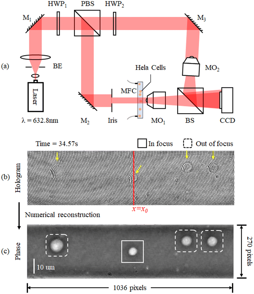

Fig. 2 The recording setup of STHD shares the same geometry with conventical DH. (a) Experimental setup. MO: microscope objective; MFC: microfluidic channel; BS: beam splitter; PBS: polarizing beam splitter; HWP: half wave plate; M: mirror; BE: beam expander. (b) A conventional hologram of flowing cells recorded with the setup shown in (a). (c) Phase map obtained via the conventional DH reconstruction process.

A sequence of 1201 holograms was captured by the system. Fig. 2(b) shows one of the holograms of the sequence. The phase-contrast map of z = 0 plane is shown in Fig. 2(c), it highlights that only one HeLa cell out of four can be considered in sharp focus. This condition occurs for all the holograms captured during the experiment, due to the absence of hydrodynamic focusing. Fig. 3(a) shows the STDH corresponding to the reference sampling column x₀ after demodulation of the horizontal fringes. In particular, the map H_0,P with P = 5 is shown. This is a 2D map that encodes 4D information, since the position of the cells in the STDH depends on time and their diffraction pattern encodes their 3D shape and position inside the LoC volume. The three-step phase shifting method is applied as described in eqn (6) to obtain the complex amplitude in the plane z = 0. The zoom-in details in Fig. 3(b) show the corresponding phase-contrast maps for the portions of STDH indicated by coloured boxes in (a). Further zoom-in details of the single cells in the white boxes in Fig. 3(b) are reported in Fig. 3(c). These show that, depending on each cell position inside the volume and its speed, four imaging cases can occur. Cells can be well sampled and in sharp focus as in the rightmost blue box in (c), meaning that they flowed in the channel centre at the nominal velocity matching eqn (4). Thanks to the use of the equivalent pixel Δx_p, 78% of the cells have been found to be well-sampled by the STDH remapping. However, most of the samples have been found to be out of focus, and a non-negligible percentage of undersampled cells has been found as well. Moreover, in all the cases an unwanted strip-like pattern corrupts the images. This is a mosaicking artefact inherently due to the use of an equivalent pixel, since two neighbour sets of P lines might correspond to capture times in which the illumination or the mean background value slightly changed. We used the proposed processing pipeline to remove all the above mentioned artefacts and to return a complex amplitude map where all the objects flowing in the LoC volume are mapped simultaneously in sharp focus and well sampled.

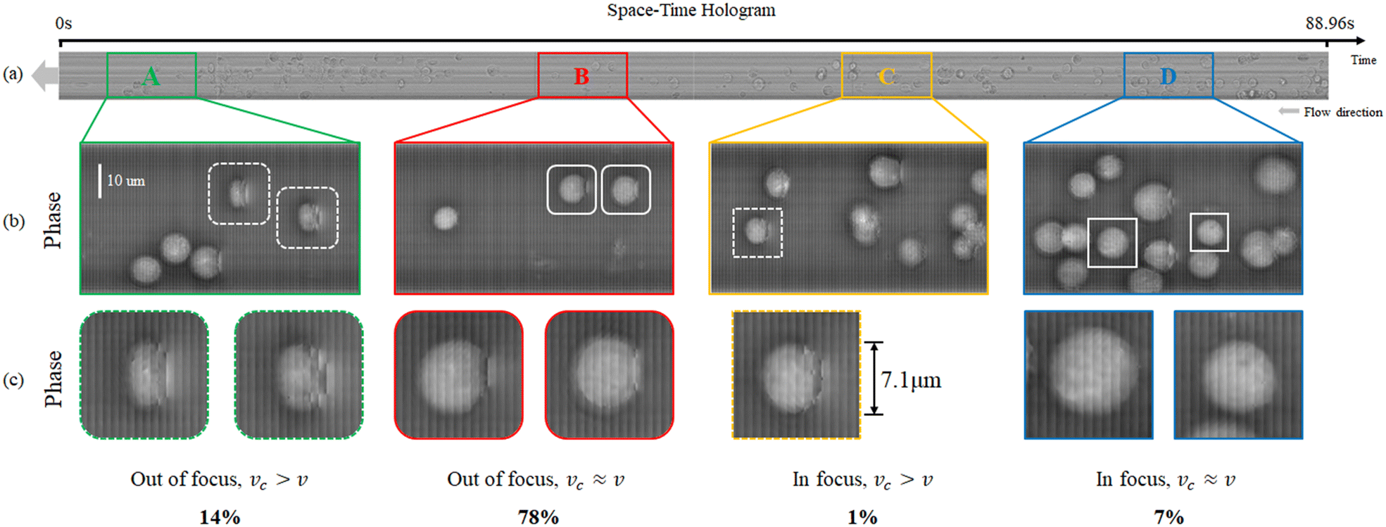Fig. 3 STDH conventional reconstruction of the experimental sequence of flowing HeLa cells. (a) STDH. (b) Phase-contrast reconstruction of the areas denoted by coloured boxes in (a). (c) Zoom-in details of the cells denoted by white boxes in (b), showing different example cases for STDH-sampling and focusing conditions.

In order to show the processing results, we selected a test portion of the long STDH FoV, where four Hela cells can be found, named here as C₁, …, C₄. Fig. 4 shows the selected portion of demodulated STDH, which corresponds to |C_A(t, y; z = 0)|. We applied the Tamura coefficient analysis to the four cells we found, to show that these occupy different positions along the optical axis. Fig. 4(a)–(e) respectively show the estimated z positions for the cells under test and the corresponding Tamura optimization curves.

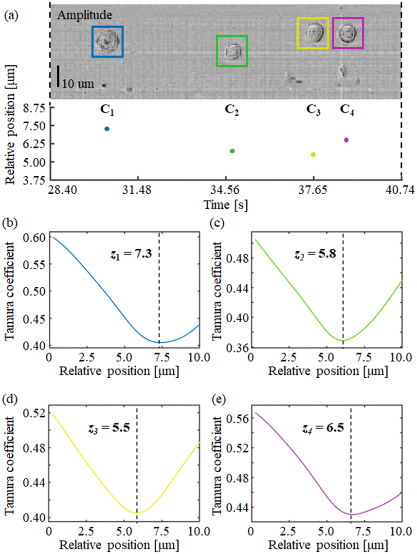Fig. 4 Tamura coefficient analysis. (a) Estimated z positions of the cells denoted by coloured boxes in the amplitude STDH reconstruction. (b–e) Plots of the Tamura coefficient as a function of the propagation distance and its minimization to estimate the best-focus position.

It is worth noticing that the Tamura coefficient has been optimized here by measuring it over a non-empty 90 × 270 sub-strip, while strip propagation at different distances is performed with a 201 × 270 strip size. In the ESI† we discuss the reason for choosing this strip size. Applying the backpropagation formula to short non-empty strips instead of the entire STDH allows saving computational time significantly, and optimizing the Tamura metric over a sub-strip ensures that the optimum focus distance is well tailored to each specific cell.

From Fig. 4(b–e) it is apparent that this choice provides Tamura plots with one single, well-defined minimum. A similar optimization process has to be carried out to remove undersampling-induced artefacts from the reconstructions using the correction factor α, after the focal planes of the cells are determined. Fig. 5 shows the (c and d) amplitudes and (a and b) phase-contrast maps for the cells C₁, C₃, and C₄. In these cases, it is apparent that conventional backpropagation (α = 1) returns images corrupted both in the sample region and the background, which is due to a residual subpixel mismatch that should be compensated for. In order to estimate the optimal value for α, we used the standard deviation of the phase-contrast values across the cell. The optimal α minimizes the standard deviation. In the ESI† we discuss the criterion behind the use of the standard deviation to estimate the α factor.

Fig. 5 Estimation of the correction factor α on cells reconstructed in focus. (a and b) Phase-contrast space-time DH maps of different cells obtained for α = 1 (no correction) and for the estimated optimum α. (c and d) Corresponding amplitude reconstructions. (e and f) Standard deviation measured over the coloured lines in (a and b) as a function of α and its minimization. (g) STDH. The area denoted by the coloured box indicates the size of each strip. (h–j) Different views of the estimated α as a function of the selected strip and the x position inside the channel. These 3D models present a complete view for the alpha factor distribution throughout the entire STDH.

Fig. 5(e and f) plot the standard deviation vs. α for the cells C₁ and C₃, measured over the coloured lines in (a) and (b), respectively. The reconstructions obtained using the optimal correction factors (i.e. α = 0.44 for C₁ and α = 0.47 for C₃) in the diffraction propagation kernel are reported in the rightmost subfigure in Fig. 5(a–d). It is apparent that the reconstruction took benefit from the introduction of the anamorphic propagation process, as the artefacts are removed in both the amplitude and phase-contrast images. In order to make the correction process automatic for the entire STDH, we measured the optimum alpha value for each strip. As discussed before, using strips instead of the entire STDH allows speeding up the estimation process, so that we are able to estimate the optimal α for each propagation distance. Fig. 5(g) shows |C_A(t, y; z = 0)| where one of the strips is highlighted with a red box.

Fig. 5(h–j) show a 3D view, and top and side views respectively of the estimated correction factor map. In Fig. 5, α is plotted as a function of the strip under test and the depth of the channel where the strip is propagated, i.e. the reconstruction distance z. By inspecting the behaviour of the correction map as a function of the channel depth, we note that the distribution of the correction factor almost symmetrically follows the distribution of the expected velocity inside the channel. In particular, we found α values approaching unity for propagation distances that image in focus objects flowing close to the top and the bottom of the channel. On the contrary, the objects flowing close to the channel middle section require much smaller α values, i.e. the equivalent pixel should be stretched more to match their speed. This result can be interpreted by considering the typical distribution of velocity that establishes inside microfluidic channels. Indeed, the cells flowing close to the middle section of the LoC are typically faster than the cells flowing close to the channel faces due to the frictional force exerted by the channel top and bottom walls.

Moreover, it is less likely to find cells flowing close to the walls, so that for those propagation distances in many strips applying a correction factor is not necessary and α can be set to unity. Since the α factor is inserted in the numerical propagation kernel, it would have no effect without propagation. For this reason, we did not report any α value when depth = 0 μm in Fig. 5(h–j). We believe that this result is a clear indication of the effectiveness of the strip-based estimation procedure, since the correction values we found well match the expected behaviour of the laminar flux establishing inside the LoC.

The result of the processing pipeline we propose is the extended DoF, extended FoV, corrected phase-contrast map shown in Fig. 6. This is an image that maps all the cells that flowed inside the chip during the experiment, in sharp focus and well sampled. In particular, the full FoV phase-contrast map is shown in Fig. 6(a) along with a plot of the correction factor applied to each strip at the best focus propagation distance. This map contains the lossless compressed information of all the cells flowing inside the channel during the 88.96 s experiment and corresponds to a video consisting of 1201 conventional digital holograms. In other words, conventional DH would require 1201 holograms to store the cells' temporal and spatial information, including phase information, velocity, and three-dimensional position. Storing these holograms would require 826 MB space. In ASTDH, just one space-time hologram is required for saving the same information, which only requires 14.3 MB space for saving.

Fig. 6 STDH phase-contrast reconstruction of the whole microfluidic experiment. (a) Average α as a function of the strip, and the corresponding corrected, extended FoV, extended DoF phase-contrast STDH map. (b and c) Enlarged details of the coloured intervals of (a), showing the samples undistorted and in sharp focus. (d) Side-by-side comparison between (right) the unprocessed STDH map of the samples I–III and (left) the result of the proposed correction pipeline.

Fig. 6(b and c) show zoom-in details corresponding to the coloured sections in (a). It is apparent that all the HeLa cells are returned in sharp focus and well sampled although they occupied different uncontrolled positions inside the LoC and they flowed at uncontrolled speed. In particular, the cells that in Fig. 3(b and c) were undersampled and out-of-focus (see e.g. the areas marked with A and B in Fig. 3(a) and the white boxes in Fig. 3(b)) are correctly imaged in Fig. 6(b and c) (see the areas marked in yellow and red). The effect of the proposed processing is more evident from Fig. 6(d–i), where we compare the conventional STDH phase mapping (Fig. 6(d, f and h)) to the novel ASTDH (Fig. 6(e, g and i)), applied to the cells marked with I–III in Fig. 6(b and c). It is worth mentioning that, in the related experiments, we did not precisely control the flow rate of the injected cells. The cells were injected freely by a syringe and thus different concentrations and velocities of cell flow are established inside the MFC. In the area of 9.63 s to 24.32 s, severe cell packing occurred due to a cell concentration exceeding 437 000 cells per ml. This caused clogging of the microfluidic channel once the cells arrive at the channel exit, which was not the expected concentration of cells in the MFC. Essentially, as for conventional DH, STDH imaging has certain limitation in terms of cell concentration. This upper concentration limit mainly depends on the size of the microfluidic channel and the cell type. For HeLa cells flowing in the 58 mm × 40 μm × 25 μm MFC, the maximum allowable cell concentration is 255 000 cells per ml. In the experiments we have shown, the initially prepared cell concentration was 155 000 cells per ml. Since the rate of cell injection was not controlled, this resulted in uneven distribution of cell concentration in the MFC. The actual concentration of cells flowing through the channel in the experiments we show goes from 38 000 to 437 000 cells per ml. Once the cell concentration exceeds the limit, the cell edge recognition as well as its reconstruction process is negatively affected. For instance, the high-density cell clusters prevent the autofocusing algorithm from giving the correct focus plane.

Conclusions

Conventional STDH maps the object in the hybrid space-time domain and retrieves the complex amplitude of objects by exploiting their motion, without using piezoelectric actuators or other external components. Using LSAs instead of 2D sensors allows capturing data at a higher frame rate and thus allows the cells to flow faster. The most natural application of STDH is the high-throughput, extended-FoV mapping of biological samples flowing inside LoC devices.^23,32,33 Besides FoV extension, conventional STDH can enhance resolution along the scanning direction, acting just like a synthetic aperture radar.³⁶ In order to ensure undistorted imaging and large DoF to map in focus at the same time all the samples flowing during a long microfluidic experiment, a proper matching has to be ensured between the sample speed and the frame rate of acquisition.^31,32 The matching condition expressed in eqn (4) has to stand in each sample image plane, which is not obtainable exactly even in ideal flow state unless hydrodynamic focusing is provided. Here we introduced the ASTDH method and a related processing pipeline well-tailored to manage the synthesis of extended-FoV, extended-DoF, STDH complex amplitude maps. The ASTDH strategy allows us to realize multi-point cells' imaging in MFCs. Moreover, it further broadens the application range of DH and realizes smart adaptation of focus and microfluidic speed. Meanwhile, it also compresses the required data storage space under the premise of ensuring the imaging resolution.

ASTDH is a solution for minimizing the artifacts of STDH while keeping all its benefits. Thus, the pixel correction factor and the extended focus optimization process are means that lead to more accurate representations of the cells' phase imaging. For the cells with different velocities and focal lengths, ASTDH allows them to be reconstructed with the same quality of cells flowing all in focus and well-sampled. This overcomes the main limitation of conventional STDH that would require a uniform flow rate. In the processing pipeline of ASDTH, we recover the subpixel mismatches by introducing a correction factor through a change of variables in the hologram back-propagation kernel. This has the effect of correcting the mismatch-induced distortion that shows up when eqn (4) does not stand for a sample. We estimate the best correction factor and propagation distance for each sample, which depend on its position inside the channel volume. These are based on the minimization of a contrast metrics measured over “sub-strips” of the longer STDH, which allows estimating optimal values tailored to each specific sample even for high density volumes. Besides, we investigated the possibility to propagate STDH-strips instead of the entire STDH to reduce the computational cost and to permit parallel computing, GPU-based, fast multicore implementations. We found that using strips of size 201 pixels allows efficient propagation while preserving the image resolution. Experiments have been carried out by imaging a bulk flow of HeLa cells flowing inside a LoC without making use of accurate flow control systems. We successfully recovered the extended FoV-DoF amplitude and phase contrast maps of all the flowing samples, which are simultaneously imaged in sharp focus. In the presented experimental results, as shown in Fig. 6, 88.96 s conventional DH recording took 826 MB space to save 1201 holograms. The ASTDH allows compressing all information included in these holograms in one single space-time hologram with 14.3 MB space. Data compression also results in saving computational time. In the case of the experiments shown in this work, we obtained a reduction of a 9.81 factor in computational time (see the ESI† for details).

Further improvements could be made to the processing pipeline to tackle the case of samples that belong to the same strip of the STDH but in different focus positions. For such cases, hologram stretching in the spatial direction or the introduction of a cubic phase plate^38,40 could solve the problem, which will be object of further investigations from our group. Moreover, deep learning-based processing could enable faster ASTDH reconstructions.^44,45 In this sense, the algorithms developed here could serve as a basis for creating an input output dataset for AI-training. We believe that ASTDH will bring benefit to all MFC-based cell imaging experiments, especially for cell identification and classification of multi-types, cell 3D tracking and counting. For most MFC-based holographic flow cytometry experiments, ASTDH can provide a stable and reliable data compression process without special setting of the recording setup. It is also worth highlighting that although the camera we used for the proposed manuscript was an area array CCD camera (this choice is discussed above), STDH allows the use of linear sensor arrays, which creates the possibility for very high-speed acquisitions of cell flow.

Conflicts of interest

P. F., V. B. and Z. W. have a pending patent concerning the method described in this manuscript.

References

1. D. Psaltis, S. R. Quake and C. Yang, Nature, 2006, 442, 381–386.
2. N. Huang, H. Zhang, M. Chung, J. Seo and K. Kurabayashi, Lab Chip, 2014, 7, 1230–1245.
3. T. O'Connor, J. Shen, B. T. Liang and B. Javidi, Opt. Lett., 2021, 46(10), 2344–2347.
4. G. Popescu, T. Ikeda, R. R. Dasari and M. S. Feld, Opt. Lett., 2006, 31(6), 775–777.
5. Y. Li, A. Mahjoubfar, C. Chen, K. Niazi, L. Pei and B. Jalali, Sci. Rep., 2019, 9(11088), 1–12.
6. Y. Zhang, M. Ouyang, A. Ray, T. Liu, J. Kong, B. Bai, D. Kim, A. Guziak, Y. Luo, A. Feizi, K. Tsai, Z. Duan, X. Liu, D. Kim, C. Cheung, S. Yalcin, H. C. Koydemir, O. B. Garner, D. Di Carlo and A. Ozcan, Light: Sci. Appl., 2019, 8(91), 1–15.
7. M. Villone, P. Memmolo, F. Merola, M. Mugnano, L. Miccio, P. L. Maffettone and P. Ferraro, Lab Chip, 2018, 18(1), 126–131.
8. D. K. Singh, C. C. Ahrens, W. Li and S. A. Vanapalli, Biomed. Opt. Express, 2017, 8(2), 536.
9. A. V. Belashov, A. A. Zhikhoreva, T. N. Belyaeva, E. S. Kornilova, A. V. Salova, I. V. Semenova and O. S. Vasyutinskii, J. Opt. Soc. Am. A, 2020, 37(2), 346–352.
10. M. Delli Priscoli, P. Memmolo, G. Ciaparrone, V. Bianco, F. Merola, L. Miccio, F. Bardozzo, D. Pirone, M. Mugnano, F. Cimmino, M. Capasso, A. Iolascon and P. Ferraro, IEEE J. Sel. Top. Quantum Electron., 2021, 27(5), 5500309.
11. M. Hejna, A. Jorapur, J. S. Song and R. L. Judson, Sci. Rep., 2017, 7, 11943.
12. T. Cacace, V. Bianco and P. Ferraro, Opt. Lasers Eng., 2020, 106188.
13. P. Memmolo, G. Aprea, V. Bianco, R. Russo, I. Andolfo, M. Mugnano, F. Merola, L. Miccio, A. Iolascon and P. Ferraro, Biosens. Bioelectron., 2022, 201(113945), 1–9.
14. Y. Zhang, H. Wang, Y. Wu, M. Tamamitsu and A. Ozcan, Opt. Lett., 2017, 42(19), 3824–3827.
15. T. Yao, R. Cao, W. Xiao, F. Pan and X. Li, J. Biophotonics, 2019, 12(7), e201800443.
16. T. Cacace, V. Bianco, M. Paturzo, P. Memmolo, M. Vassalli, M. Fraldi, G. Mensitieri and P. Ferraro, Lab Chip, 2018, 18(13), 1921–1927.
17. L. Xin, W. Xiao, L. Che, J. Liu, L. Miccio, V. Bianco, P. Memmolo, P. Ferraro, X. Li and F. Pan, ACS Omega, 2021, 6(46), 31046–31057.
18. W. Xiao, L. Xin, R. Cao, X. Wu, R. Tian, L. Che, L. Sun, P. Ferraro and F. Pan, Lab Chip, 2021, 21(7), 1385–1394.
19. X. Heng, D. Erickson, L. R. Baugh, Z. Yaqoob, P. W. Sternberg, D. Psaltis and C. Yang, Lab Chip, 2006, 6, 1274–1276.
20. V. Bianco, M. Paturzo and P. Ferraro, Opt. Express, 2014, 22(19), 22328–22339.
21. N. C. Pégard, M. L. Toth, M. Driscoll and J. W. Fleischer, Lab Chip, 2014, 14(23), 4447–4450.
22. V. Micó, C. Ferreira and J. García, Opt. Express, 2012, 20(9), 9382.
23. V. Bianco, M. Paturzo, V. Marchesano, I. Gallotta, E. Di Schiavi and P. Ferraro, Lab Chip, 2015, 15(9), 2117–2124.
24. J. H. Massig, Opt. Lett., 2002, 27(24), 2179–2181.
25. Optical superresolution, ed. Z. Zalevsky and D. Mendlovic, Springer-Verlag New York Inc., 2004, ISBN: 0387005919.
26. T. C. Poon, J. Holography Speckle, 2004, 1, 6–25.
27. D. W. E. Noom, D. E. B. Flaes, E. Labordus, K. S. E. Eikema and S. Witte, Opt. Express, 2014, 22(25), 30504–30511.
28. D. Pirone, M. Mugnano, P. Memmolo, F. Merola, G. Lama, R. Castaldo, L. Miccio, V. Bianco, S. Grilli and P. Ferraro, Nano Lett., 2021, 21(14), 5958–5966.
29. B. Mandracchia, J. Son and S. Jia, Lab Chip, 2021, 21, 489–493.
30. P. Song, C. Guo, S. Jiang, T. Wang, P. Hu, D. Hu, Z. Zhang, B. Feng and G. Zheng, Lab Chip, 2021, 21, 4549–4556.
31. B. Mandracchia, V. Bianco, Z. Wang, M. Mugnano, A. Bramanti, M. Paturzo and P. Ferraro, Lab Chip, 2017, 17(16), 2831–2838.
32. H. Yamada, A. Hirotsu, D. Yamashita, O. Yasuhiko, T. Yamauchi, T. Kayou, H. Suzuki, S. Okazaki, H. Kikuchi, H. Takeuchi and Y. Ueda, Biomed. Opt. Express, 2020, 11(4), 2213–2223.
33. C. Ai and J. C. Wyant, Appl. Opt., 1987, 26(6), 1112–1116.
34. N. T. Shaked, Y. Zhu, M. T. Rinehart and A. Wax, Opt. Express, 2009, 17(18), 15585–15591.
35. M. K. Kim, Opt. Lett., 2020, 45(3), 784–786.
36. V. Bianco, Z. Wang, Y. Cui, M. Paturzo and P. Ferraro, Opt. Lett., 2018, 43(17), 4248–4251.
37. P. W. M. Tsang, T. Poon and J. Liu, Sci. Rep., 2016, 6(21636), 1–7.
38. F. Del Giudice, G. Romeo, G. D'Avino, F. Greco, P. A. Netti and P. L. Maffettone, Lab Chip, 2013, 13, 4263–4271.
39. T. Colomb, N. Pavillon, J. Kühn, E. Cuche, C. Depeursinge and Y. Emery, Opt. Lett., 2010, 35(11), 1840–1842.
40. M. Matrecano, M. Paturzo and P. Ferraro, Opt. Eng., 2014, 53(11), 112317.
41. S. De Nicola, P. Ferraro, A. Finizio and G. Pierattini, Opt. Lett., 2001, 26, 974–976.
42. P. Memmolo, V. Bianco, M. Paturzo and P. Ferraro, Proc. IEEE, 2016, 105(5), 892–905.
43. L. Jin, Y. Tang, Y. Wu, J. B. Coole, M. T. Tan, X. Zhao, H. Badaoui, J. T. Robinson, M. D. Williams, A. M. Gillenwater, R. R. Richards-Kortum and A. Veeraraghavan, Proc. Natl. Acad. Sci. U. S. A., 2020, 117(52), 33051–33060.
44. D. M. Siu, K. C. Lee, B. M. Chung, J. S. Wong, G. Zheng and K. K. Tsia, Lab Chip, 2023, 23.
45. D. Pirone, D. Sirico, L. Miccio, V. Bianco, M. Mugnano, P. Ferraro and P. Memmolo, Lab Chip, 2022, 22(4), 793–804.

---

Footnote

† Electronic supplementary information (ESI) available. See DOI: https://doi.org/10.1039/d3lc00063j

---