Urban-scale analysis of the seasonal trend of stabilized-Criegee intermediates and their effect on sulphate formation in the Greater Tokyo Area†
Received
5th July 2023
, Accepted 20th October 2023
First published on 24th October 2023
Abstract
We conducted an urban-scale analysis of the contribution of gas phase stabilized-Criegee intermediates (sCIs) to atmospheric sulphate aerosol (SO42−) formation across four seasons in the Greater Tokyo Area (GTA) using the regional chemical transport model, the community multiscale air quality modelling (CMAQ) system. We analysed the seasonal and temporal trend of sCI formation in three areas: Tokyo Bay (urban), suburban, and mountainous areas. In all three areas, the sCI concentrations were high in the morning (7 a.m.) and early evening (6 p.m.) owing to the high frequency of vigorous traffic activities causing intense alkene emissions. The results suggest that more than 90% of the sCIs generated in the target areas are consumed by the unimolecular decomposition of sCIs themselves or by reactions with water, which are consistent with estimates from previous kinetic analysis studies targeting other regions. The contribution of sCIs to SO42− formation estimated in this study was a maximum of 0.25% in the rural area, which is approximately 10-fold lower than that of previous studies. The results of the sCI loss pathway analysis suggested that the unimolecular decomposition of sCIs and the reaction between sCIs and water contribute comparably to the loss of sCIs, which caused less of an effect of sCIs on SO42− formation compared with that in previous studies.
Environmental significance
In this study, the contribution of stabilized-Criegee intermediates (sCIs) to sulphate aerosol formation (SO42−) was evaluated by the regional-chemical transport model targeted urban, suburban, and rural areas of the Greater Tokyo Area of Japan. This study makes a significant contribution to the literature because we proved that sCI-derived SO42− formation is not as significant as that estimated by the previous study in the calculated region and thus, we updated the regional-scale sCIs contribution to SO42− formation in the Greater Tokyo Area. Further, we analysed the seasonal and timely trend of sCI formation, the effect of sCI-derived SO42− on radiative forcing, etc., all of which are expected to be useful to understand “Criegee chemistry” on a regional scale by both scientists and policymakers.
|
Introduction
Stabilized-Criegee intermediates (sCIs) are strong oxidants for trace gases, which are generated by alkene and diene (hereafter called alkene) ozonolysis.1–5 Recently, numerous studies have performed kinetic analyses of sCIs to elucidate their environmental fate in the atmosphere.6–10 sCIs are either lost by unimolecular decomposition or bimolecular reactions in the atmosphere. In unimolecular decomposition, sCIs decompose to produce OH depending on their structure, whereas sCIs react with trace gases, water vapour (water monomer and water dimer), sulphur dioxide (SO2), nitrogen dioxide (NO2), nitric acid (HNO3), carbon monoxide, alcohols, aldehydes, and organic acids in bimolecular reactions. Mauldin et al. reported that sCIs play a non-negligible role in the oxidation of SO2 and contribute to the formation of sulphate aerosol (SO42−) in the atmosphere.5
Regional chemical transport model calculations, including sCI reactions, were conducted to evaluate the sCI contribution to SO42− formation. Itahashi et al.11,12 calculated the sCI contribution to SO42− formation over a winter haze episode in the Greater Tokyo Area (GTA), Japan used the community multiscale air quality modelling (CMAQ) system and concluded that the sCI reactions have a contribution of SO42− concentration enhancement.11,12 Liu et al. also reported that sCI reactions affected the SO42− concentration during a persistent summer air pollution episode in Beijing–Tianjin–Hebei, China evaluated by a WRF-Chem model.13 Several studies suggested that the reaction of sCIs with water would significantly affect SO42− formation via the oxidation of SO2 by sCIs by 1 to 10%, depending on which value is used for the rate constant of H2O reaction.14–16 These studies did not consider the unimolecular decomposition of sCIs in their fate. Cox et al. summarized the estimated atmospheric concentration of sCIs in the U.K. from kinetic analysis studies including sCI + water reactions and the unimolecular decomposition of sCIs,17 and they showed that most of the sCIs are scavenged by water reactions or unimolecular decompositions in the urban, suburban, and rural areas of the U.K.
In this study, we evaluated the contribution of Criegee chemistry to the formation of SO42− in the GTA using the regional air quality model. The atmospheric concentrations of sCIs were estimated and the SO42− concentrations induced by the sCI reactions were deduced.
Recently, a quantum chemical study calculated the loss reaction rates of many types of sCIs and showed that sCIs derived from biogenic volatile organic compounds (BVOCs) are mainly lost by unimolecular decomposition.18 The study also quantified the sCI contribution to the atmosphere using a global chemical transport model. The annual averaged ambient sCI concentration was estimated to be approximately 1000 molecules per cm3 in most parts of the world, including Japan. In addition, they found that the sCI contribution to SO42− formation is 5% or less at the global scale, except for selected regions, such as tropical rain forests. However, the seasonal difference in the regional sCI concentrations and their contribution to SO42− formation is not well understood.
In this study, we evaluated the sCI concentrations and their contribution to SO42− formation over four seasons in the GTA, Japan in 2015. We used a chemical transport model with generation reactions for 14 sCIs, including the sCIs derived from alkenes, and 7 sCI loss reaction processes, including unimolecular decomposition. In addition, negative radiative forcing of the SO42− derived from the sCIs was also estimated.
Methodology
Chemical transport modelling
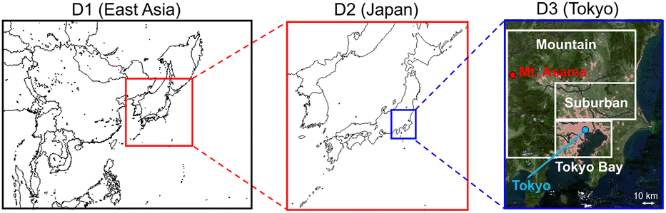
CMAQ v5.2.1 (ref. 19) was used to simulate the air quality calculations; the detailed schemes for CMAQ are described in Table S1 of the ESI.† There were three domains calculated in this study, which are described in Fig. 1: East Asia (D1: 45 × 45 km), Japan (D2: 15 × 15 km), and the GTA (D3: 5 × 5 km). The GTA is located in the Kanto Plain, which consists of the cities of Tokyo and Saitama, as well as Kanagawa, Chiba, Ibaraki, Gunma, and Tochigi prefectures. The population of the GTA is approximately 43 million, i.e., one-third of Japan,20 which is concentrated around Tokyo. Flat land, including suburban areas, spreads out in the southern part of the Kanto Plain. Several highways, including the metropolitan expressway, pass through the study site. The Keihin industrial region, which is the largest industrial region in Japan, and the Keiyo industrial area are located in Tokyo Bay. These regions are characterised by high emissions of anthropogenic volatile organic compounds (AVOCs) due to vigorous industrial activity; more than half of the SO2 emissions in GTA derive from Tokyo Bay. There are mountainous areas across the northern and western parts of the Kanto Plain, where biogenic VOC (BVOC) emissions are a dominant component of the VOC emissions. The analysed D3 domain is categorized into three areas: Tokyo Bay, suburban areas, and mountain areas.
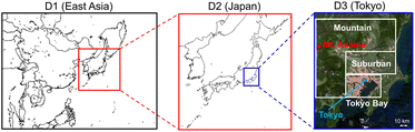 |
| | Fig. 1 Calculated domains for D1 (East Asia), D2 (Japan), and D3 (Greater Tokyo Area (GTA)). D3 is divided into three areas: Tokyo Bay, suburban, and mountain areas. | |
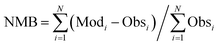
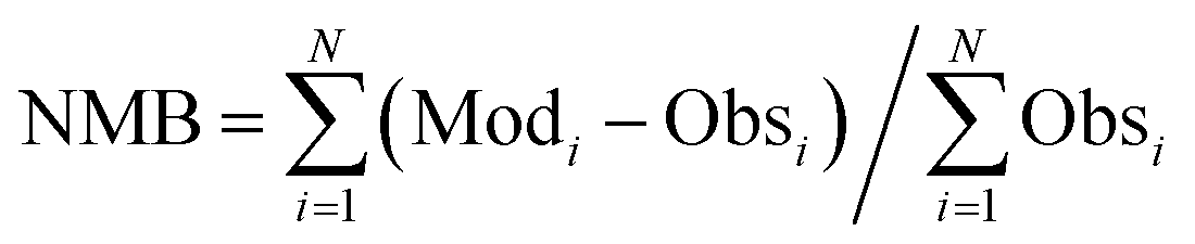
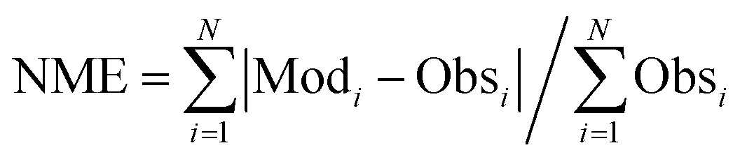
The calculated term was the entire year of 2015 (from Jan. 1 to Dec. 31); winter (Jan. 10 to Feb. 15), spring (May 10 to Jun. 15), summer (Jul. 10 to Aug. 15), and winter (Oct. 10 to Nov. 15) were chosen as the analysis terms in this study. The first 5 days of each season were treated as the spinoff term of the calculation. The meteorological parameters calculated by the weather research and forecasting (WRF) model version 3.7.1 (ref. 21) were applied to the CMAQ calculation. The emissions inventories provided by Chatani et al. were applied to anthropogenic emissions both inside and outside of Japan.22 MEGANv2.1 was used to calculate the emissions inventory of BVOC emissions.23 Further details on the input parameters for the meteorology and emissions inventories of the primary air pollutants are described in Table S1,† which is based on a previous study.24 SAPRC-07 was used as the gas-phase chemical mechanism,25 coupled with the AERO6 aerosol chemistry module.26 The gas-phase chemical mechanism was modified by incorporating sCI chemistry, which is described in the next section. The modelling performance for SO42−, the targeted component of this study, was evaluated using three indicators such as the normalized mean bias (NMB), normalized mean error (NME), and correlation coefficient (R), of which NMB and NME are defined in eqn (1) and (2) as follows:
| |  | (1) |
| |  | (2) |
where subscript
i is the pairing of
N observations (Obs) and calculations (Mod) from each site and time. Emery
et al. proposed values of NMB, NME, and
R that are required for the chemical transport modelling.
27 In terms of SO
42−, Emery
et al. proposed that the required criteria of NMB, NME, and
R are <±0.30, <0.50, and >0.40, respectively while the required goal of NMB, NME, and
R are <±0.10, <0.35, and >0.70, respectively.
Incorporation of gas phase chemical mechanisms of stabilized-Criegee intermediates in the chemical transport model
Vereecken et al. evaluated a wide variety of reaction rate constants for sCI-related reactions derived from alkene ozonolysis by quantum chemical calculations coupled with transition state theory.18 Following Vereecken et al., in this study, a total of 245 sCI-related reactions (including 26 sCI-generation reactions (including E- and Z-isomers) listed in Table S2,† unimolecular decompositions listed in Table S3,† sCI-loss reactions with water monomer (H2O) and water dimer ((H2O)2) listed in Tables S4 and S5,† and sCI reactions with SO2 and NO2, among others, listed in Tables S6–S9†) were incorporated into the chemical mechanism of SAPRC-07. The rate constants and chemical mechanisms of sCI-generation, as listed in Table S2 of the ESI,† were derived from the Master Chemical Mechanism version 3.3.1.28,29 Some sCIs hold structural isomers (E-sCI and Z-sCI), such that we assumed that the branching ratio of sCI generation for each isomer was the same (1![[thin space (1/6-em)]](https://www.rsc.org/images/entities/char_2009.gif) :1) owing to the lack of information on the branching ratio of alkene ozonolysis to E-sCI and Z-sCI. As previous studies have reported the importance of H2O and (H2O)2 for the loss of sCIs,14–16 as well as the fact that the ratio of H2O and (H2O)2 is strongly dependent on the ambient temperature, the temperature dependency was considered for the reaction of sCIs with water (H2O and (H2O)2).18 The temperature dependency for unimolecular decomposition was also considered because the parameters necessary for the temperature dependency calculation were also available in the literature.18 The rate constants of the remaining reactions were fixed to 298 K. Further details on the incorporated sCI reactions are described in the following sections. Detailed structures of the 26 sCIs are shown in Fig. S1 of the ESI.†
:1) owing to the lack of information on the branching ratio of alkene ozonolysis to E-sCI and Z-sCI. As previous studies have reported the importance of H2O and (H2O)2 for the loss of sCIs,14–16 as well as the fact that the ratio of H2O and (H2O)2 is strongly dependent on the ambient temperature, the temperature dependency was considered for the reaction of sCIs with water (H2O and (H2O)2).18 The temperature dependency for unimolecular decomposition was also considered because the parameters necessary for the temperature dependency calculation were also available in the literature.18 The rate constants of the remaining reactions were fixed to 298 K. Further details on the incorporated sCI reactions are described in the following sections. Detailed structures of the 26 sCIs are shown in Fig. S1 of the ESI.†
Unimolecular decomposition of sCIs
The unimolecular decomposition mechanism of sCIs was investigated by several studies using both experimental and theoretical methods.18,30–32 In this study, we applied the rate constants for unimolecular decomposition proposed by Vereecken et al.18 The unimolecular decomposition rates evaluated by transition state theory coupled with quantum chemical calculation were applied, as listed in Table S3.† The 1,3-ring closure and 1,4-H-migration are the main unimolecular decomposition pathways of sCIs, which were considered in this study.
Loss of sCIs via reaction with water monomers and water dimers
Water is known as the main contributor to the loss of sCIs from the atmosphere, which accounts for more than half of the total sCI consumption. The rate constants of sCIs with H2O were cited from a previous study.18 The reaction products of sCIs with H2O and sCIs with (H2O)2 were assumed to be the same for the products of SCI1 (CH2OO) with H2O and (H2O)2.33 Previous studies have suggested that the rate of the sCI-loss reaction with (H2O)2 is 2–3 orders of magnitude higher than that with H2O. According to Khan et al.,4 the ratio of [(H2O)2] to [H2O] ([(H2O)2]/[H2O]) is less than 0.01, but the ratio should change with atmospheric conditions, such as the ambient temperature. To the best of our knowledge, no studies have considered detailed time variations in the [(H2O)2]/[H2O] in the chemical transport model. In this study, [(H2O)2]/[H2O] was determined by the thermodynamical approach. In the atmosphere, H2O and (H2O)2 coexist under thermal equilibrium conditions, as follows:
The equilibrium constant, Kw, of reaction (R1) is as follows:
| | | Kw(T) = [(H2O)2]/[H2O]2 | (3) |
The sCIs loss reaction by (H2O)2 is as follows:
| | 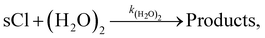 | (R2) |
where
k(H
2O)
2 is the rate constant of reaction
(R2). We assumed that the temperature dependence of the rate constant
k(H
2O)
2 is exhibited by the modified Arrhenius equation, as follows:
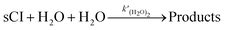
| | | k(H2O)2(T) = A1(T/300)B1exp(−Ea1/RT), | (4) |
where
A1 is the pre-exponential factor,
B1 is the constant for the temperature variable, and
Ea1 is the activation energy. Meanwhile, to introduce the reactions of sCIs with (H
2O)
2 in the SAPRC-07 chemical mechanism of CMAQ, the reaction was transformed to the following expression
(R3) by dividing (H
2O)
2 as two H
2O:
| |  | (R3) |
where

is the rate constant of reaction
(R3). The temperature dependence of the rate constant is as follows:
| | 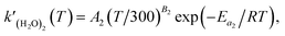 | (5) |
where
A2 and
B2 correspond to those of
eqn (2). Combining
eqn (3)–(5), the rate constant of

is expressed as follows:
| |  | (6) |
Previous studies formulated Kw and k(H2O)2 based on experimental results.34 We obtained the Arrhenius parameters of A2, B2, and Ea2 by fitting them to the experimental results. These processes were required because CMAQ requires the users to input kinetic parameters with the Arrhenius equation when introducing new chemical mechanisms.
sCI reactions with SO2, NO2, HNO3, and organic acids
The main purpose of this study is to evaluate the atmospheric effects of SO42− formation induced by sCIs at the urban scale. Aside from SO2, sCIs react with other active air pollutants. In this study, the oxidation reactions of SO2, NO2, HNO3, organic acids (formic acid (HCOOH), acetic acid (CH3COOH), and organic acids with a high carbon number (RCOOH)) were considered as the chemical mechanism of the sCI reactions, as listed in Tables S6–S9.† In terms of sCI reactions with SO2 and organic acids, the reported difference in structural isomers (E-sCI and Z-sCI) and rate constants was applied in this study. In contrast, in terms of sCI reactions with NO2 and HNO3, only limited rate constants were available; all rate constants for both sCIs with NO2 and HNO3 were treated as the same value obtained from Raghunath et al.35 The products of the reaction between sCIs and organic acids were assumed to be the same for the unimolecular decomposition of sCIs listed in Table S9,† which were obtained from Welz et al.36 and Chhantyal-Pun et al.37 Notably, while several studies have assumed that the product of sCIs + NO2 is NO3,37,38 Caravan et al. found that the main product of sCIs + NO2 could be the sCI-NO2 adduct with an upper limit of about ∼30% decomposing to NO3 and ketones (aldehyde).39 Therefore, the actual products are uncertain. However, because of this uncertainty and the emphasis of this study on SO2 products, we assumed that all the products from sCIs + NO2 reactions were NO3.
Results
Modelling performance for the prediction of SO42− concentration
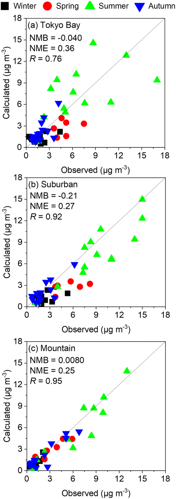
Fig. 2 shows the comparison of observed and calculated results of SO42− at the three analysed sites: Tokyo Bay, suburban, and mountain areas in the four analysed seasons without incorporation of the chemistry of sCIs. Except for the value of NMB of suburban, all the plots in the three analysed sites met the goal of modelling performance proposed by Emery et al.27 (the definitions of the indicators are described in the Methodology). The value of NMB for suburban also met the criteria of modelling performance. For these reasons, the calculated SO42− concentration in the analysed domain reproduced the observed results well and can be applied for the kinetic analysis of sCI-related chemistry. Despite the facts of well modelling performance, the calculated SO42− concentration underestimated the observed results in winter and spring seasons for Tokyo Bay and suburban areas by ∼50%. The fact of underestimation should be considered when analysing the effect of sCIs on SO42− formation in winter and spring seasons.
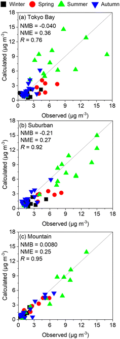 |
| | Fig. 2 Comparison between observed and calculated SO42− concentrations in the four seasons of the three analysed sites: (a) Tokyo Bay, (b) suburban, and (c) mountain. | |
Ambient concentration of sCIs in the Tokyo Bay area
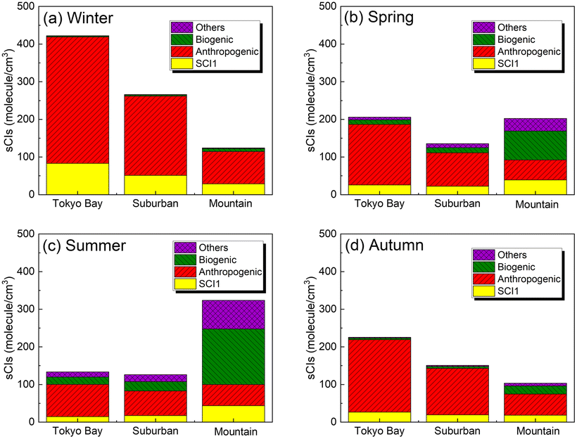
Fig. 3 shows the speciation of the sCI concentration for Tokyo Bay, suburban, and mountain areas for each season after introducing 245 sCI-related reactions to SAPRC-07. The distribution of the sCI concentration is shown in Fig. S2.† According to Fig. 3, the total sCI concentration was less than 500 molecules per cm3 during all seasons, consistent with a previous study conducted using the global chemical transport model, which introduced unimolecular decompositions of sCIs.18 In winter and autumn, the average sCI concentration was high in Tokyo Bay (maximum of 420 molecules per cm3). As previously mentioned, the AVOC emissions in Tokyo Bay are higher than in other areas because of the high density of population, traffic, and industrial activities. Further, lower rate constants for unimolecular decomposition led to slower sCI consumption, owing to the lower temperature and lower reaction rate constant of sCIs with water under the low water vapour concentration in winter and autumn. Further details on the loss process of sCIs are discussed in the next section. In spring and summer, the sCI concentration was high in the mountain area, being 320 molecules per cm3 in summer while reaching 600 molecules per cm3 at the highest level. In spring and summer, intense sunlight and high temperatures cause BVOC emissions from forests, which enhance ozone formation, a precursor of sCIs.
 |
| | Fig. 3 Speciation of sCIs (originating from formaldehyde oxide (SCI1), anthropogenic sources, biogenic sources, and others) in the three areas: Tokyo Bay, suburban, and mountain areas in the calculated domain for (a) winter, (b) spring, (c) summer, and (d) autumn. As SCI1 is generated from both anthropogenic and biogenic sources, it is treated separately. The sCIs generated from ‘other’ sources are produced from the intermediate alkenes in the atmosphere, such as methyl vinyl ketone, generated from isoprene ozonolysis. | |
The entire annual average of the diurnal changes in the sCI concentrations in the three areas is shown in Fig. 4(a). The sCI concentrations showed peaks at 7 a.m. and 6 p.m., exhibiting the highest levels of 350, 250, and 300 molecules per cm3 in Tokyo Bay, suburban, and mountain areas, respectively. In contrast, the sCI concentrations decreased just before dawn and daytime, showing the lowest levels of 150, 100, and 100 molecules per cm3 in Tokyo Bay, suburban, and mountain areas, respectively. Fig. 4(b) and (c) show the diurnal change in the alkene and ozone concentrations, which are the precursors of sCIs. Ozone had high concentration at around noon. In contrast, the alkene concentration peaked at 7 a.m. and 6 p.m., showing a similar trend in the sCIs, as shown in Fig. 4(a). This suggests that the sCI concentration is mainly dependent on the concentration of alkenes in the Tokyo Metropolitan area. Here, 7 a.m. and 6 p.m. correspond to the commuting hours; the high concentration of alkenes derives from vehicle emissions.40,41 The concentration of alkenes in the mountain area did not show significant changes during commuting hours compared with the two other areas because the main source of alkenes in the mountain area is BVOC emissions from vegetation, which is predominantly independent of human activities. Fig. S3 to S8† show the spatial distributions of the calculated SO2, O3, VOCs, and water as the reference for basic information in this study.
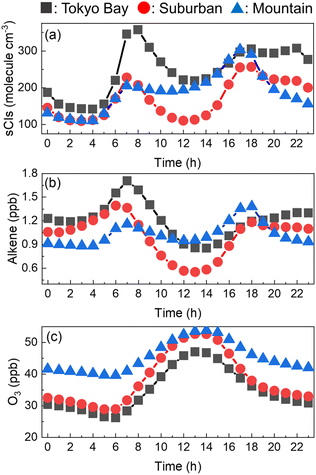 |
| | Fig. 4 Hourly concentrations of (a) sCIs, (b) alkene, and (c) O3 in the three areas. The concentrations were averaged for the four seasons. | |
Effect of sCIs on surface SO42− formation in the Greater Tokyo Area (GTA)
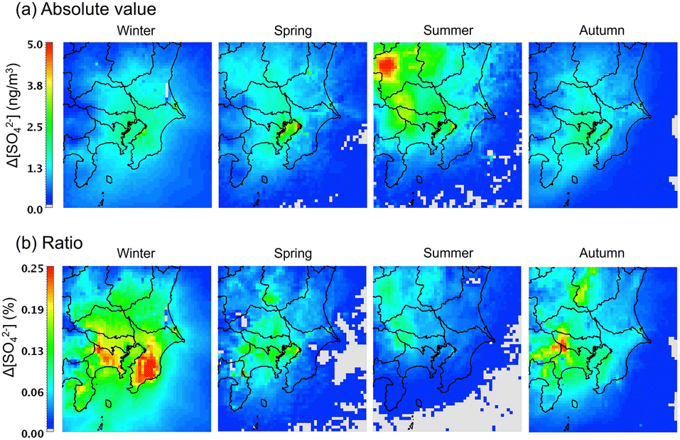
The change in the surface concentration of SO42− in the D3 domain after introducing the sCI reactions to the gas-phase chemical mechanism is shown in Fig. 5. The concentrations of SO42− in Tokyo Bay during all seasons are affected by the sCI reactions. The Tokyo Bay area contains a significant amount of anthropogenic emission sources of both alkene and SO2, especially in the coastal area, as shown in Fig. S9 and S11.† In the summer, a high increase in the SO42− concentration was obtained at the north-west site of D3, which was caused by intense SO2 emissions from the volcanic activity at Mt. Asama. The increase in the SO42− concentration after introducing the sCI reactions was 1.0 to 5.0 ng m−3, which corresponds to 0.05–0.25% of the total SO42− concentration. Itahashi et al. evaluated the effect of sCI reactions on the SO42− concentration using CMAQ in the same region as this study. They reported 10 to 50 ng m−3 (0.5–3%) contributions to SO42− formation in the winter season, of which the value had a maximum 10-fold higher than that obtained in this study. Itahashi et al. did not include two important sCI-loss processes, i.e., the unimolecular decomposition and reaction with (H2O)2, which may lead to an overestimation of the effect of the sCI reactions on SO42− formation.11 The contribution of the sCI reactions to the SO42− formation reached a maximum of 5.0 ng m−3 (or 0.25% of the total SO42−), which is not critical to the total SO42− concentration on the ground surface of the GTA region. As stated in the previous section, the calculated SO42− underestimated the observed results in winter and spring seasons for Tokyo Bay and suburban regions by ∼50%. Nevertheless, the contribution of sCIs to SO42− formation is at most ∼0.3% according to Fig. 5(b), and we conclude that sCI reactions are not the main reasons for the underestimation of SO42− in the calculated region.
 |
| | Fig. 5 Change in the SO42− surface concentrations after introducing sCI reactions in SAPRC-07. (a) Absolute concentration and (b) percentage of concentration change. | |
Discussion
Effect of sCI-derived sulphate aerosol (SO42−) on radiative forcing
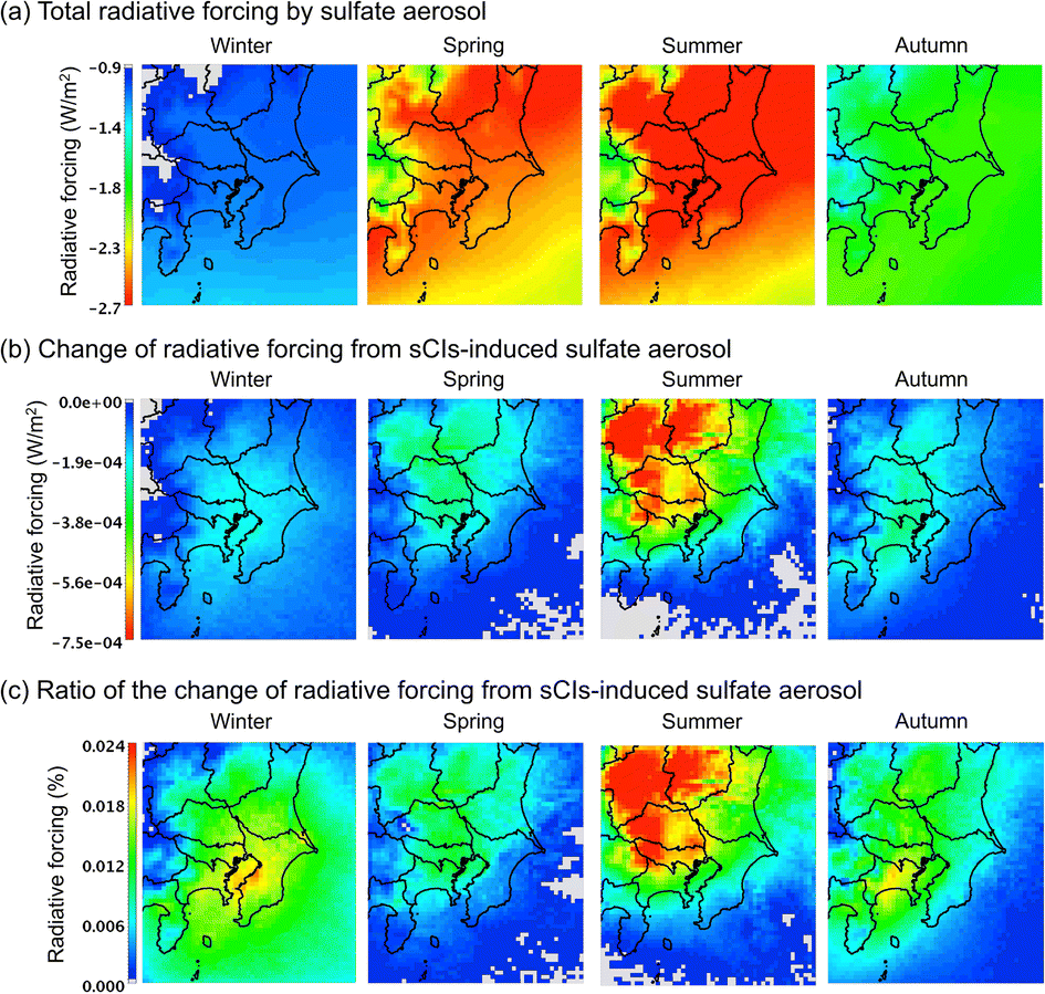
The results above suggest that the effect of sCIs on the surface concentration of SO42− is not critical to the total SO42− concentration in all seasons in GTA. While the surface concentration of SO42− is important for evaluating air pollution, which has detrimental effects on humans and crops, the column integrated concentration of SO42− is important for evaluating radiative forcing (as well as the long-range transport of SO42−), which is associated with global warming (SO42− is characterised by negative radiation forcing). According to Boucher et al., the radiative forcing, RF (W), induced by SO42− is proportional to the column weight of SO42−, Wcolsulphate (g), as follows:42| | | RF = RsulphateWcolsulphate, | (7) |
where Rsulphate is a constant (W g−1); according to Boucher et al., Rsulphate = 150 was applied. Fig. 6 shows the results of the calculated radiative forcing. The decrease in the radiative forcing by SO42− is high during warm seasons, i.e., late spring and summer, and low in the cold seasons, i.e., winter and late autumn. The concentration of SO42− is high in the warm seasons because of the high concentration of OH radicals due to the intense sunlight, high temperature, and humidity, in which SO2 was rapidly transformed to SO42−.43Fig. 6(b) shows the contribution of sCI-derived SO42− to the decrease in radiative forcing. The decrease in radiative forcing caused by sCI-derived SO42− was high in the summer season. The western and north-western regions of the D3 domain especially showed a high contribution from negative radiative forcing. The western area of D3 is mountainous, which causes high BVOC emissions, while the north-western area contains a volcano (Mt. Asama); these land features enhance SO42− formation, leading to higher negative radiative forcing. The decrease in radiative forcing due to sCI-derived SO42− reached a maximum of 7.5 × 10⁻⁴ W m−2, which corresponded to a relative change from the total SO42− radiative forcing of 0.024%. The radiative forcing calculated in this study was significantly smaller than that in a previous study of ∼0.1 W m−2, which was calculated without considering the sCI unimolecular decomposition and the reaction of sCIs with (H2O)2.44
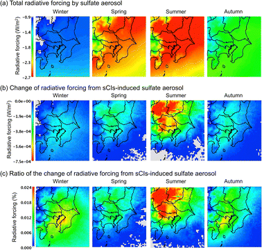 |
| | Fig. 6 Calculated radiative forcing on the Tokyo metropolitan area in the four seasons for (a) the total radiative forcing, (b) radiative forcing from sCI-derived SO42−, and (c) ratio of the contribution of sCI-derived SO42− to radiative forcing. | |
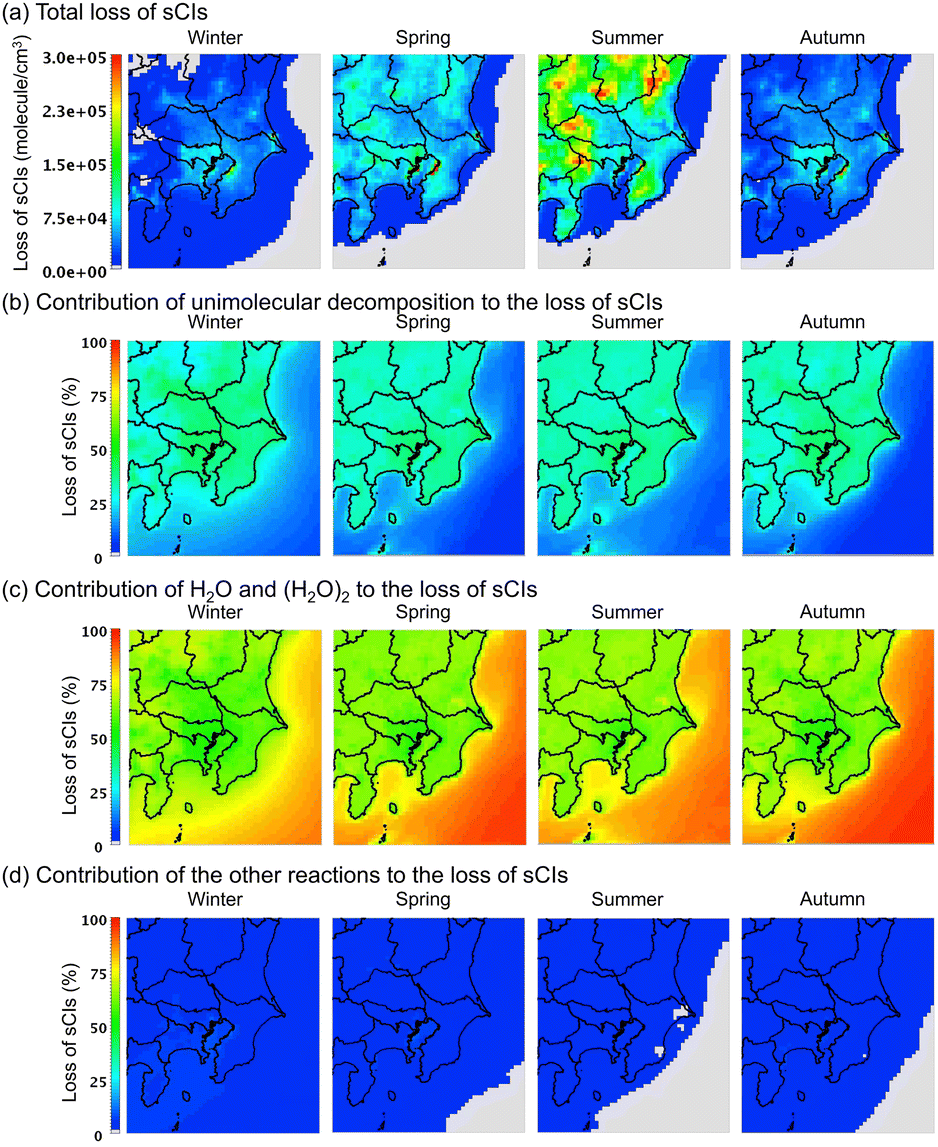
Contribution from loss of sCIs by unimolecular decomposition and reaction with water
Fig. 7 shows the average distribution of the sCI-loss rate across the four seasons in the GTA for the (a) total loss, (b) loss by unimolecular decomposition, (c) loss by reaction with water molecules, and (d) loss by other reactions. According to Fig. 7(a), the total loss rate in the sCI reactions was high in summer, followed by spring. In the summer and spring, the sCI-loss rates increased due to high temperatures, which led to a high rate constant for the unimolecular decomposition of sCIs. The high temperatures also increased the already high concentration of water vapour in the atmosphere, which enhanced the reaction of sCIs with water monomers and dimers. According to Fig. 7(b) and (c), sCI unimolecular decomposition and the reaction of sCIs with water molecules contributed to more than 90% of the sCI loss. Higher water concentrations in the summer season would enhance the removal reaction of sCIs with water. Nevertheless, according to Fig. 7(c), the contributions of water in the four seasons were almost equal. This is because the rate constants of the sCIs with the water monomers and dimers showed negative temperature dependences.34 Aside from this, the equilibrium of the water monomers and dimers shown in reaction (R1) is inclined to the monomer side towards an increase in temperature.
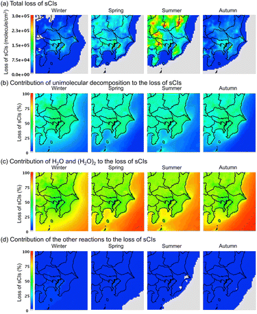 |
| | Fig. 7 Seasonal averaged distribution of sCI loss in the four seasons for the (a) total amount, (b) contribution of unimolecular decomposition to total sCI loss, (c) contribution of water to total sCI loss, and (d) contribution of other reactions (e.g., with SO2 and NO2, among others) to the total sCI loss. The detailed values of sCI-loss for each sCI species are listed in Table S10.† | |
Comparison of sCI concentrations with other countries
Trend of sCI concentration.
In this study, the average sCI concentration in the GTA was 100–400 molecules per cm3, with a maximum of over 1000 molecules per cm3 in industrial areas during winter. Cox et al. reported the sCI concentration in the urban, suburban, and rural areas of the United Kingdom.17 They found an average sCI concentration of 350–500 molecules per cm3, with a maximum of more than 1000 molecules per cm3 in the summer season in the rural area, i.e., the same order of magnitude reported in this study. Further, Cox et al. reported that during the daytime, the sCI concentration was 2–3-fold higher in the morning and evening than other hours, which is also a similar trend found in this study.17
Fig. 8 shows the relationship between the sCI concentration and (a) ozone, (b) alkene, and (c) multiplying the ozone and alkene concentrations. From Fig. 8(a) and (b), the ozone and alkene concentrations are independently non-linearly correlated with the sCI concentration. Fig. 8(c) shows the linear relationship between alkene × ozone and sCIs, indicating that the sCIs could be generated within the balance of alkene and ozone. Further, according to Fig. 8(c), the slopes of the regression lines in the summer and spring are lower than those of winter and autumn, indicating that the loss rate of sCIs in summer and spring is higher than that in winter and autumn. This can be attributed to unimolecular decomposition and reactions with water.
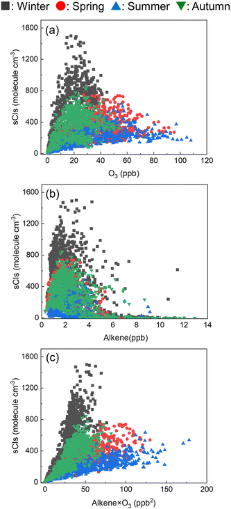 |
| | Fig. 8 Correlation between the sCI concentration and (a) O3, (b) alkene, and (c) O3 × alkene in Tokyo. | |
Seasonal trend in sCI species.
The type of sCI in the atmosphere varies depending on the season and location. According to the results of this study, the contribution of ZSCI2 in SCIs, which is generated from propene ozonolysis, reached 40% in winter and autumn while that of ESCI8, which is generated from isoprene ozonolysis, was 22% in the summer in the mountain area. According to a previous study targeting the U.K.,17 ZSCI2 accounts for more than 70% of the roadside in urban, suburban, and rural areas in winter, as well as 25–75% in the summer season. In the summer season in rural U.K., ESCI9, ESCI10, and ZSCI10, which are generated from isoprene and pinene ozonolysis, account for 29% of the total sCIs. In terms of other countries, while the contribution of ZSCI2 reaches 45% in Mexico City, which is characterised by a significant amount of AVOCs,18 ESCI8 accounts for 42% in the Amazon owing to high isoprene emissions.18 Furthermore, ZSCI10 and ZSCI11 account for most of the sCIs in the Sierra Nevada, U.S.A.18 The main global sCI from anthropogenic alkene ozonolysis is ZSCI2, which is generated from propene ozonolysis. In contrast, sCIs from BVOC ozonolysis vary with the local forest type.
Details on sCI-loss reactions.
As previously discussed, the contribution of unimolecular decomposition of sCIs is less than 50% while the reaction of sCIs with water contributes more than 50% and accounts for most of the sCI reactions in the atmosphere. According to a previous study targeting the U.K.,17 the contribution of sCI unimolecular decomposition was 43–47% and that of the reaction of sCIs with H2O and (H2O)2 was 51–54% in winter. The contribution of the unimolecular decomposition of sCIs in summer was 49–57% and that of the reaction of sCIs with water was 37–47%; thus, the unimolecular decomposition of sCIs and the reaction of sCIs with water were also dominant in the U.K. In the UK, owing to relative humidity increases in winter,45 the ratio of the water reaction to sCIs increased compared with that of summer. Further, the ratios of the unimolecular decomposition to the water reaction of sCIs in Amazonia, Mexico City, Sierra Nevada (U.S.A.), and Hohenpeissenberg (Germany) were estimated to be 54%/38%, 53%/32%, 58%/32%, and 53%/43%, respectively, all of which are on the same order of magnitude of the results of this study. However, the results for other countries tend to show a higher contribution of unimolecular decomposition of sCIs than that of the reaction of sCIs with H2O and (H2O)2.18 While these four places are located in the interior area, the GTA is surrounded by the ocean, which has relatively higher humidity. The contribution of the reaction of sCIs with H2O and (H2O)2 may increase here than in other places.
Effect of sCIs on OH formation.
Anglada et al. suggested the potential importance of sCIs in OH formation and its influence on atmospheric oxidation.46 Fig. S12† shows the difference (%) in OH concentration before and after introducing sCI-chemistry into the chemical mechanism of SAPRC-07 in the four seasons of the targeted domain. It is estimated that the OH concentrations increase by at least approximately 4% in all the seasons, and by up to 8% in winter. The OH is directly produced by the unimolecular decomposition of sCIs, bimolecular reactions of sCIs + HNO3, etc., and these reactions occur not only during the daytime but also at night, when the total OH concentration is low. These factors eventually increased the contribution of sCI on OH formation in the GTA. The increase in OH also contributes to the increase in SO42− formation through the direct oxidation of SO2 by OH. Fig. S13† shows the ratio of the SO42− formation rate between the increase in OH (Δ[OH]) and the increase in sCIs (Δ[CI]). In the winter season, the formation of SO42− is governed by the oxidation of SO2 by increasing OH, whereas in spring and summer seasons the formation of SO42− is contributed by both sCIs and the increase of OH. In autumn, most of the SO42− is increased by increasing OH. The contribution of OH increase is related to Tokyo Bay. Suburban and mountain areas hold forests and trees that emit BVOCs contributing to a high production of OH, whereas Tokyo Bay is an urban area that has less BVOC emission. Therefore, the effect of the increase of OH through sCI chemistry is more sensitive in Tokyo Bay than that in suburban and mountain areas, showing the relevant contribution of the increase of OH to the formation of SO42−. In conclusion, the enhancement of the formation of SO42− after the incorporation of sCI chemistry results from the oxidation reaction of SO2 by sCIs and the increased OH. In addition, the oxidation of SO2 by the increased OH contributes much more to the formation of SO42− than the direct sCI oxidation of SO2.
Summary
The effect of gas-phase sCIs on SO42− formation in the GTA was evaluated using chemical transport modelling coupled with more than 200 chemical reactions related to Criegee intermediates proposed by previous studies. The results suggested that the maximum contribution of sCIs to SO42− formation accounts for 5.0 ng m−3, which corresponds to 0.25% of the total SO42− concentration, indicating lower effects of sCIs in the targeted domain compared with previous studies.11,12 The difference in the results derives from the incorporation of unimolecular decomposition of sCIs and the reaction with (H2O)2 in this study. The SO42− formation from sCIs contributes to a 0.024% decrease in radiative forcing. The results of the sCI loss pathway analysis showed that the consumption of sCIs via reactions with water and unimolecular decay of sCIs contributes more than 90% of all sCI reactions. Therefore, most of the sCIs are consumed by those two reaction paths. This trend in the sCI fate in the atmosphere is comparable to previous studies, which targeted other regions.17,18 The results of this study provide an update on the regional-scale effect of sCIs on SO42− formation in the Japanese region.
Author contributions
Yuya Nakamura – carried out numerical simulation, performed analysis, wrote the draft paper, Hiroo Hata – proposed the research concept, prepared meteorological inputs and emission inventories, verified for accuracy, and Kenichi Tonokura – supervision, verified the work for accuracy.
Conflicts of interest
There are no conflicts to declare.
Acknowledgements
This study was partly supported by a Grant-in-Aid for Scientific Research (C) from the Japan Society for the Promotion of Science (JSPS), Grant Number 21K12286. Part of this study was conducted as Type II joint research between the National Institute for Environmental Studies and the local environmental research institutes of Japan. The authors also thank Dr Steven Kraines of the National Research Institute of Advanced Industrial Science and Technology for proofreading some of the English.
References
- C. A. Taatjes, D. E. Shallcross and C. J. Percival, Phys. Chem. Chem. Phys., 2014, 16(5), 1704–1718 RSC.
- G. T. Drozd, T. Kurtén, N. M. Donahue and M. I. Lester, J. Phys. Chem. A, 2017, 121(32), 6036–6045 CrossRef CAS PubMed.
- Z. Hassan, M. Stahlberger, N. Rosenbaum and S. Bräse, Angew Chem. Int. Ed. Engl., 2021, 60(28), 15138–15152 CrossRef CAS PubMed.
- H. A. M. Khan, J. C. Percival, L. R. Caravan, A. C. Taatjes and E. D. Shallcross, Environ. Sci.: Processes Impacts, 2018, 20, 437 RSC.
- R. L. Mauldin III, T. Berndt, M. Sipilä, P. Paasonen, T. Petäjä, S. Kim, T. Kurtén, F. Stratmann, V.-M. Kerminen and M. Kulmala, Nature, 2012, 488, 193–196 CrossRef PubMed.
- J. Qiu and K. Tonokura, Chem. Phys. Lett., 2019, 737, 100019 CrossRef.
- M. J. Newland, A. R. Rickard, M. S. Alam, L. Vereecken, A. Muñoz, M. Ródenas and W. J. Bloss, Phys. Chem. Chem. Phys., 2015, 17(6), 4076–4088 RSC.
- J. P. Hakala and N. M. Donahue, J. Phys. Chem. A, 2016, 120(14), 2173–2178 CrossRef CAS PubMed.
- E. V. Avzianova and P. A. Ariya, Int. J. Chem. Kinet., 2002, 34(12), 678–684 CrossRef CAS.
- M. J. Newland, B. S. Nelson, A. Muñoz, M. Ródenas, T. Vera, J. Tárrega and A. R. Rickard, Phys. Chem. Chem. Phys., 2020, 22(24), 13698–13706 RSC.
- S. Itahashi, K. Yamaji, S. Chatani and H. Hayami, Atmosphere, 2019, 10(9), 544 CrossRef CAS.
- S. Itahashi, R. Uchida, K. Yamaji and S. Chatani, Atmos. Environ.: X, 2021, 12, 100123 CAS.
- L. Liu, N. Bei, J. Wu, S. Liu, J. Zhou, X. Li, Q. Yang, T. Feng, J. Cao, X. Tie and G. Li, Atmos. Chem. Phys., 2019, 19(21), 13341–13354 CrossRef CAS.
- T. R. Lewis, M. A. Blitz, D. E. Heard and P. W. Seakins, Phys. Chem. Chem. Phys., 2015, 17(7), 4859–4863 RSC.
- T. Berndt, T. Jokinen, M. Sipilä, R. L. Mauldin III, H. Herrmann, F. Stratmann, H. Junninen and M. Kulmala, Atmos. Environ., 2014, 89, 603–612 CrossRef CAS.
- G. Sarwar, H. Simon, K. Fahey, R. Mathur, W. S. Goliff and W. R. Stockwell, Atmos. Environ., 2014, 85, 204–214 CrossRef CAS.
- R. A. Cox, M. Ammann, J. N. Crowley, H. Herrmann, M. E. Jenkin, V. F. McNeill, A. Mellouki, J. Troe and T. J. Wallington, Atmos. Chem. Phys., 2020, 20(21), 13497–13519 CrossRef CAS.
- L. Vereecken, A. Novelli and D. Taraborrelli, Phys. Chem. Chem. Phys., 2017, 19(47), 31599–31612 RSC.
- Community modeling and analysis system webpage: https://www.cmascenter.org/cmaq/, accessed May 31 2023.
- Ministry of Internal Affairs and Communications webpage: https://www.soumu.go.jp/english/index.html, accessed May 31 2023.
- WRF model users' page: https://www2.mmm.ucar.edu/wrf/users/, accessed May 31 2023.
- S. Chatani, K. Yamaji, T. Sakurai, S. Itahashi, H. Shimadera, K. Kitayama and H. Hayami, Atmosphere, 2018, 9(1), 19 CrossRef.
- A. B. Guenther, X. Jiang, C. L. Heald, T. Sakulyanontvittaya, T. Duhl, L. K. Emmons and X. Wang, Geosci. Model Dev., 2012, 5(6), 1471–1492 CrossRef.
- H. Hata, K. Inoue, K. Kokuryo and K. Tonokura, Environ. Sci. Technol., 2020, 54(10), 5947–5953 CrossRef CAS PubMed.
- W. P. L. Carter, Atmos. Environ., 2010, 44(40), 5324–5335 CrossRef CAS.
- F. S. Binkowski and S. J. Roselle, J. Geophys. Res.: Atmos., 2003, 108(D6), 4183 CrossRef.
- C. Emery, Z. Liu, A. G. Russell, M. T. Odman, G. Yarwood and N. Kumar, J. Air Waste Manage. Assoc., 2017, 67(5), 582–598 CrossRef CAS PubMed.
- S. M. Saunders, M. E. Jenkin, R. G. Derwent and M. J. Pilling, Atmos. Chem. Phys., 2003, 3(1), 161–180 CrossRef CAS.
- M. E. Jenkin, S. M. Saunders, V. Wagner and M. J. Pilling, Atmos. Chem. Phys., 2003, 3(1), 181–193 CrossRef CAS.
- M. I. Lester and S. J. Klippenstein, Acc. Chem. Res., 2018, 51(4), 978–985 CrossRef CAS PubMed.
- R. Chhantyal-Pun, O. Welz, J. D. Savee, A. J. Eskola, E. P. F. Lee, L. Blacker, H. R. Hill, M. Ashcroft, M. A. H. Khan, G. C. Lloyd-Jones, L. Evans, B. Rotavera, H. Huang, D. L. Osborn, D. K. W. Mok, J. M. Dyke, D. E. Shallcross, C. J. Percival, A. J. Orr-Ewing and C. A. Taatjes, J. Phys. Chem. A, 2017, 121(1), 4–15 CrossRef CAS PubMed.
- Y.-H. Lin, C. Yin, K. Takahashi and J. M. Lin Jr, Commun. Chem., 2021, 4, 12 CrossRef CAS PubMed.
- L. Sheps, B. Rotavera, A. J. Eskola, D. L. Osborn, C. A. Taatjes, K. Au, D. E. Shallcross, M. A. H. Khan and C. J. Percival, Phys. Chem. Chem. Phys., 2017, 19(33), 21970–21979 RSC.
- M. C. Smith, C. H. Chang, W. Chao, L. C. Lin, K. Takahashi, K. A. Boering and J. J. Lin, J. Phys. Chem. Lett., 2015, 6(14), 2708–2713 CrossRef CAS PubMed.
- P. Raghunath, Y. P. Lee and M. C. Lin, J. Phys. Chem. A, 2017, 121(20), 3871–3878 CrossRef CAS PubMed.
- O. Welz, A. J. Eskola, L. Sheps, B. Rotavera, J. D. Savee, A. M. Scheer, D. L. Osborn, D. Lowe, A. Murray Booth, P. Xiao, M. Anwar, H. Khan, C. J. Percival, D. E. Shallcross and C. A. Taatjes, Angew Chem. Int. Ed. Engl., 2014, 53(18), 4547–4550 CrossRef CAS PubMed.
- R. Chhantyal-Pun, B. Rotavera, M. R. McGillen, M. A. H. Khan, A. J. Eskola, R. L. Caravan, L. Blacker, D. P. Tew, D. L. Osborn, C. J. Percival, C. A. Taatjes, D. E. Shallcross and A. J. Orr-Ewing, ACS Earth Space Chem., 2018, 2(8), 833–842 CrossRef CAS.
- D. Meidan, S. S. Brown and Y. Rudich, ACS Earth Space Chem., 2017, 1, 288–298 CrossRef CAS.
- R. Caravan, M. A. H. Khan, B. Rotavera, E. Papajak, I. O. Antonov, M.-W. Chen, K. Au, W. Chao, D. L. Osborn, J.-M. Lin Jr, C. J. Percival, D. E. Shallcross and C. A. Taatjes, Faraday Discuss., 2017, 200, 313–330 RSC.
- K. F. Ho, S. C. Lee, H. Guo and W. Y. Tsai, Sci. Total Environ., 2004, 322(1–3), 155–166 CrossRef CAS PubMed.
- E. Velasco, B. Lamb, H. Westberg, E. Allwine, G. Sosa, J. L. Arriaga-Colina, B. T. Jobson, M. L. Alexander, P. Prazeller, W. B. Knighton, T. M. Rogers, M. Grutter, S. C. Herndon, C. E. Kolb, M. Zavala, B. de Foy, R. Volkamer, L. T. Molina and M. J. Molina, Atmos. Chem. Phys., 2007, 7(2), 329–353 CrossRef CAS.
- O. Boucher and M. Pham, Geophys. Res. Lett., 2002, 29(9), 22 CrossRef.
- J. F. Meagher, E. M. Bailey and M. Luria, J. Geophys. Res., 1983, 88(C2), 1525–1527 CrossRef CAS.
- J. Li, Q. Ying, B. Yi and P. Yang, Atmos. Environ., 2013, 79, 442–447 CrossRef CAS.
- Current Results – Weather and Science Facts: https://www.currentresults.com/.
- J. M. Anglada, P. Aplincourt, J. M. Bofill and D. Cremer, ChemPhysChem, 2002, 3(2), 215–221 CrossRef CAS PubMed.
|
| This journal is © The Royal Society of Chemistry 2023 |
Click here to see how this site uses Cookies. View our privacy policy here. 
 Open Access Article
 This Open Access Article is licensed under a
  a,
Hiroo
Hata
a,
Hiroo
Hata

 is the rate constant of reaction (R3). The temperature dependence of the rate constant is as follows:
 is expressed as follows: