
 Open Access Article
 This Open Access Article is licensed under a Creative Commons Attribution-Non Commercial 3.0 Unported Licence
Real world ultrafine particle emission factors for road-traffic derived from multi-year urban flux measurements using eddy covariance
Agnes
Straaten
 ,
Minh-Hien
Nguyen
and
Stephan
Weber
*
,
Minh-Hien
Nguyen
and
Stephan
Weber
*
Climatology and Environmental Meteorology, Institute of Geoecology, Technische Universität Braunschweig, Langer Kamp 19c, 38106 Braunschweig, Germany. E-mail: s.weber@tu-braunschweig.de
First published on 3rd August 2023
Abstract
Vehicular traffic is an important source of ultrafine particles in urban areas. The emission strength may be quantified using particle emission factors (EF) which are an important input to air-quality models such as dispersion or chemical transport models. We quantified particle EFs for a mixed traffic fleet from size-resolved particle number flux measurements in the size range 10 nm < Dp < 200 nm utilizing the eddy covariance technique at an urban site in Berlin, Germany over the time period from 2017–2020. Particle EFs were calculated using a linear regression approach of particle number fluxes vs. traffic intensity. For the 3 year observation period the average total particle number emission for the mixed fleet  was 2.80 × 10¹⁴ veh−1 km−1. The strongest particle emission occurred in the nucleation mode (Dp < 30 nm), i.e. 69% of total mixed fleet particle emission. A multiple regression analysis for light (LDV) and heavy duty vehicles (HDV) indicated higher EFHDV by a factor of 11.2 for ultrafine particles (Dp < 100 nm) than EFLDV, and a factor 9.8 for nucleation mode particles. The eddy covariance particle flux measurements proved a powerful approach to quantify size-resolved particle EFs over multiple years.
Environmental significanceElevated urban concentrations of ultrafine particles (UFP) are mainly due to significant emission from vehicular road traffic. The emission strength of UFP may be quantified using particle emission factors (EF) which are an important input to air-quality models. Due to the variation of influencing factors such as vehicle type, driving patterns, or specific traffic situations, reported EF span a wide range of values and therefore increase uncertainty of modelled concentration estimates. We derived EF from 3 years of micrometeorological particle number flux observations representing a real-world urban mixed traffic fleet. About 2/3 of traffic particle emission occurred in the nucleation mode <30 nm. Heavy duty vehicles emitted about 11 times more particles than light duty vehicles. Such longer-term observations certainly help to understand variation in EF and to monitor effects of the modernisation of the traffic fleet. |
1 Introduction
Cities are characterised by high number concentrations of airborne particles, typically with a share of more than 80–90% of ultrafine particles (UFP, diameter DP < 100 nm) in the total number concentration of particles.1 Vehicular road traffic is reported to be the dominant source of UFP in urban areas, mainly due to significant tailpipe emission of particles in the nucleation size range Dp < 30 nm.2–4 Although evidence on the impact of UFP on human health from epidemiological studies is inconclusive5 there are clear indications for human health threats due to elevated UFP exposure.6 Hence, the European Commission recently issued a revision of the air quality directive, in which regular monitoring of UFP number concentrations at selected sites throughout Europe is proposed in order to collect data for health-related and epidemiological research on a routine basis.7The emission strength of particles from vehicular road traffic is usually quantified using particle emission factors (EF) for specific vehicle types or mixed fleets such as composed of light and heavy duty vehicles, or cars of different fuel types. A number-based EF specifies the particle number as emitted per vehicle (veh) and unit distance or unit of burned fuel, e.g. particles per veh per km or particles per kg of fuel. Particle EFs in different diameter size ranges have been quantified using methods either under controlled laboratory conditions or in real-world situations such as car tunnels, street canyons, along motorways or in urban areas.8–12 The most common methods to derive EFs are dynamometer measurements, different gaseous traffic tracer methods (e.g. NOx tracer method), on-road chasing experiments, inverse modelling approaches or using eddy-covariance flux data.13–16 The EFs are important input data to air quality models, e.g. dispersion models, to implement the source strength of road traffic and subsequently calculate atmospheric transformation and spatial distribution of particle concentrations.
Reported real-world emission factors, however, span a wide range of values, mainly due to the variation of influencing factors in the different research studies such as fuel and vehicle type, driving patterns, vehicle age, topography of the study area, meteorological conditions, or the measured particle size range.17,18 Many studies also look at relatively short study periods of a few weeks or months and therefore may not capture the range of variation in influencing factors, e.g. meteorological conditions.16 Hence, to better understand the variation of particle EFs, longer observation periods in urban areas are vital. Eddy covariance is a technique to measure the vertical surface-atmosphere exchange of energy or pollutants by a direct approach, i.e. without assumptions about the turbulent state of the atmosphere. In combination with traffic data, the measured surface-layer turbulent transport of particles can be utilised to derive emission factors representing the flux source area upwind of the eddy covariance site. Depending on the measurement height and the turbulent state of the atmosphere, the flux source area typically covers a surface area of about 102 to 104 m.19 This provides the opportunity to quantify urban road traffic EFs under real-world conditions from measured particle fluxes, i.e. for a mixed vehicle fleet with varying traffic driving patterns such as free flowing traffic or congested conditions. Multi-year measurements enable to study temporal variation, which might point to emission trends in the mixed vehicle fleet or help to assess the effects of traffic mitigation strategies.
In the present study, a 3 year data set of size-resolved particle fluxes from an urban site in Berlin covering the time period 2017–2020 was used to derive traffic emission factors for particles in the size range 10 nm < Dp < 200 nm. To date, only very few studies are available which report findings from multiple years of eddy covariance particle fluxes and provide size-resolved information on particle EFs.20 We hypothesise that long-term eddy-covariance observations are a very valuable method to derive particle EFs for a mixed urban fleet covering a large variation of boundary conditions such as driving patterns, turbulent transport and meteorological conditions. We aim to quantify a ‘typical’ mixed-fleet road traffic emission factor which is representative for urban Berlin or other large German cities with similar fleet compositions. Hence, we excluded periods with ‘non-typical’ traffic situations such as weekends or holidays and focussed our analysis on the case of an average weekday situation. Particle EFs are reported for size integrated number concentrations such as ultrafine and total particle number concentrations as well as for concentrations in the nucleation, Aitken and accumulation modes.
2 Material and methods
2.1 Study site
Size-resolved particle number fluxes were measured at rooftop of the main building of Technische Universität Berlin, Germany in the time period from April 2017–March 2020 (Fig. 1). The site is part of the Urban Climate Observatory Berlin21 and located at a height of 47 m above ground level (agl). The mean building height in the vicinity of the site amounts to approximately 18 m above ground level.22 An impression of the site surroundings is depicted in the Appendix (Fig. 8). To the north of the site, the main road ‘Straβe des 17. Juni’ with an average daily traffic (ADT) of 42![[thin space (1/6-em)]](https://www.rsc.org/images/entities/char_2009.gif) 700 vehicles per day (average from Monday–Thursday, data source: ref. 23) is located, which is one of the busiest roads in the vicinity of the site.
700 vehicles per day (average from Monday–Thursday, data source: ref. 23) is located, which is one of the busiest roads in the vicinity of the site.
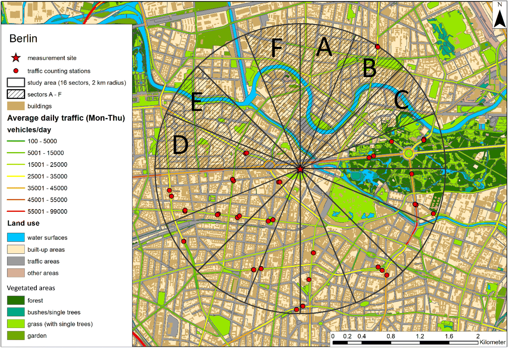 | ||
| Fig. 1 Study area in Berlin within a radius of 2 km around the flux site. Please note that the average daily traffic (Mon–Thu) is only shown for major roads. Traffic data of the traffic counting stations were provided by the Senate Department for the Environment, Urban Mobility, Consumer Protection and Climate Action of the Berlin city administration (map data sources: ref. 23). Sectors A–F indicate the areas for calculation of particle EFs (cf. Section 2.4). | ||
The study area was defined as a 2 km radius around the site, since this area contains the 80% contour line of the flux source area in every single of the three observation years as determined by flux source area modelling (cf.20). For the study area, data of 22 automatic traffic counting stations were available from the Senate Department for the Environment, Urban Mobility, Consumer Protection and Climate Action of the Berlin city administration (red dots in Fig. 1). The data set included continuous traffic counts of the respective road cross-section at each site from the period April 2017–March 2020 for the mixed vehicle fleet and separate counts for heavy (HDV) and light duty vehicles including passenger cars (LDV). The absolute maximum daily sums of traffic counts at the 22 sites range between 30150 vehicles per day and 68630 vehicles per day over the study period. The average fraction of HDVs in the study area accounted for about 6–7% of total traffic counts. These traffic time series were used to calculate the spatially distributed traffic activity data for estimation of the particle emission factors (cf. Section 2.4).
2.2 Instrumentation
Particle number flux measurements were conducted with a fast electrical mobility particle sizer (Engine Exhaust Particle Sizer Spectrometer, EEPS 3090, TSI Inc., Minnesota, USA) and a 3D ultrasonic anemometer (USA-1, Metek GmbH, Elmshorn, Germany). Data from both devices were synchronously sampled with a frequency of 10 Hz and logged by a desktop computer. The ultrasonic anemometer and the sample inlet for particle number size distribution (PNSD) measurements were mounted at the top of a 10 m high hydraulic mast which was located at rooftop. This resulted in a measurement height of about 57 m agl. The sample air was transported through a stainless steel tube with an inner diameter of 0.01 m and a flow rate of 10 L min−1 towards the EEPS and was dried using a Nafion dryer (MD-700, length 0.9 m, Perma Pure LLC). Although the particle size spectrum of the EEPS ranges from 5.6 to 560 nm, the size range for particle number flux measurements was limited to 10 < Dp < 200 nm. This size range reduction was necessary due to the gap-filling procedure according to Meyer-Kornblum et al.24 which results in increased uncertainties in the boundary regions of the PNSD (cf. Section 2.2). For further details on the gap-filling procedure and the measurement setup, the authors refer to ref. 20 and 24.2.3 Data handling for particle flux calculation
The PNSDs required for particle number flux calculation were first corrected for particle losses in the sampling line (and the Nafion dryer).25 Particle number concentrations in specific size channels of the PNSD below the associated EEPS minimum threshold value were interpolated using a cubic natural spline interpolation method.24 If too many concentration readings within a PNSD (10 nm < Dp < 200 nm) were below the minimum thresholds (>9 gaps) or were in neighbouring size channels (>5 contiguous gaps), this PNSD was rejected. Overall, 14% of the PNSD data were rejected because of too many gaps in the PNSD. From the remaining 86% of PNSDs, 0.6% were without any gaps and did not require gap-filling, whereas 85.4% of data were gap-filled. According to the analysis of the gap-filling method using the natural spline interpolation24 the uncertainty in total number concentrations arising from the gap-filling procedure is about 10% for the size range 10 < Dp < 200 nm. Our analysis did not point to any bias in the method which tended to a systematic under- or overestimation of particle concentrations by the gap-filling.20 For these PNSDs size-integrated number concentrations were calculated in order to process particle number fluxes, i.e. total particle number concentration (TNC, 10 nm < Dp < 200 nm), ultrafine particle number concentration (UFP, 10 nm < Dp < 100 nm), nucleation mode particles (NUC, 10 nm < Dp < 30 nm), Aitken mode particles (AIT, 30 nm < Dp < 100 nm), and accumulation mode particles (ACC, 100 nm < Dp < 200 nm).Several corrections and quality checks were applied for particle number flux calculation, which was performed using EddyPro® v6.2.2 software. The tolerance for missing samples was set to 20%, meaning that there had to be at least 80% data availability in each half-hour period. Furthermore, particle and wind data were checked for plausibility range and spikes were removed.26 Spectral corrections regarding high-pass and low-pass filter effects were applied using the methods of Moncrieff et al.27,28. In addition, double coordinate rotation for tilt correction, linear detrending and a time lag correction by covariance maximisation within a specific time lag window (9 s ± 4.5 s) were used. Underestimation of particle number flux due to EEPS response time was calculated and corrected,29 while data quality was characterised according to Foken et al.30. In that respect, particle fluxes with quality flags >6 were discarded. The resulting particle number fluxes are subject to the following sign convention: emission fluxes have a positive sign and are directed to the atmosphere, whereas deposition fluxes are negative and directed to the surface. For further details on data handling, quality control, or data assurance the reader is referred to Straaten et al.20.
2.4 Preparation of the traffic data set
For the determination of particle emission factors using eddy covariance fluxes, a specific data set with traffic information in the unit veh km m−2 s−1 (traffic activity, TA) is needed.15 To gather this information, the spatial distribution of ADT (data source: ref. 23) in each of the 16 sectors within the 2 km radius (Fig. 1), was combined with hourly traffic data from 22 traffic counting stations located in the study area (Fig. 2).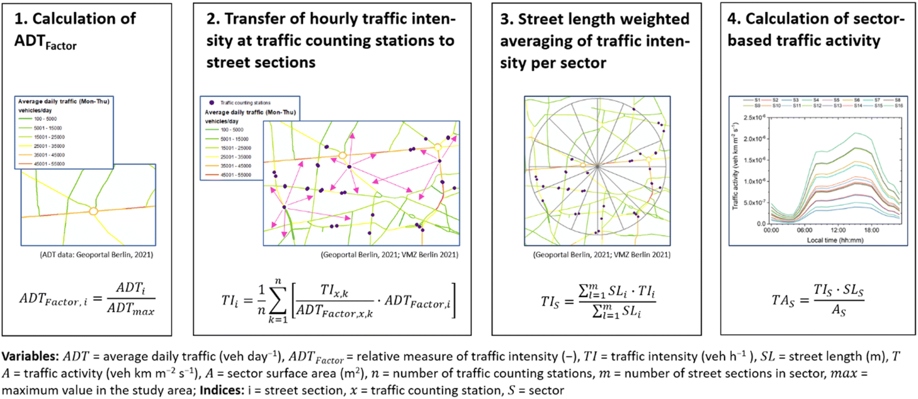 | ||
| Fig. 2 Workflow of the required procedures to calculate a traffic data set for quantification of particle emission factors. | ||
In the first step, a quantity ADTFactor was obtained for each street section i of the ADT data set in the 2 km radius using eqn (1)
 | (1) |
 | (2) |
For the analysis of particle emission factors on a sector basis, TI had to be determined at the sector level. Hence, the TIi of m street sections within a sector S were arithmetically averaged, and weighted by its street length (SLi).
 | (3) |
In the last step, the sector-based traffic activity (TAS) was calculated using the total street length of the sector (SLS) and the sector area (AS).
 | (4) |
The resulting data set included hourly traffic data of TA for the three measurement years for each of the 16 sectors of the study area.
2.5 Quantification of road-traffic emission factors
To quantify road traffic related particle emission factors from eddy covariance observations, particle number emission fluxes (i.e. positive fluxes, cf. Section 2.2) were subject to linear regression versus sector-wise traffic activity TA for wind sectors strongly influenced by traffic. The linear fit to the data according to eqn (5)15| F = EFmf × TA + F0 | (5) |
| F = EFLDV × TALDV + EFHDV × TAHDV + F0 | (6) |
In order to derive robust particle emission factors for urban road traffic, wind sectors must be characterised by significant traffic activity. Here, we selected wind directions sectors which were characterised by high average particle emission fluxes during the three study years (cf.Fig. 9a) and have >20% of traffic land use in the sector flux source area.20 The sectors meeting this requirements are located to the west and north of the study site (cf.Fig. 1, 270°–67.5°). However, the NW sector located between sectors E and F (315°–337.5°) was excluded due to the occurrence of distinct deposition fluxes (Fig. 9b). We argue that particle deposition and emission fluxes may appear simultaneously in the urban boundary layer. Thus, a strong emission flux may be reduced by simultaneously occurring particle deposition. Since deposition and emission fluxes in this sector were in the same order of magnitude (cf.Fig. 9), we excluded this sector from further analysis. As a result, six of the 16 sectors (sectors A–F; Fig. 1) were selected for the determination of particle emission factors. However, the remaining sectors were used to evaluate the robustness of EFmf (cf. Section 3.2). Time periods with lower traffic intensity such as weekends and vacation periods were discarded in order to calculate road traffic emission factors for typical weekday traffic conditions.
Particle emission factors were quantified sector-wise, i.e. for each wind direction sector A–F specifically, to study the variation of EFmf due to different traffic activity per sector. Subsequently, emission factors were also calculated as an average emission factor for the six sectors A–F  to characterise the typical road traffic emission for the study area. The tailpipe and non-tailpipe particle emission from vehicles will be subject to different physical and chemical aerosol transformation processes during turbulent atmospheric transport such as coagulation, condensation and others (e.g.31). As this study determines emission factors using particle fluxes observed at a receptor site (i.e. the eddy covariance site at 57 m agl) we define the resulting emission factor as an effective real-world particle emission factor for road traffic which is not corrected for atmospheric transformation processes.
3 Results
3.1 Sectoral analysis
Traffic-related particle emission factors in the selected wind sectors A–F were in the range 1.54 × 10¹⁴ to 3.47 × 10¹⁴ veh−1 km−1 (Fig. 3 and Table 1). The lowest emission factor occurred in sector D, whereas the highest emission factors were evident in sectors C and F. The EFmf for binned particle fluxes were in a range of 1.45 × 10¹⁴ to 3.80 × 10¹⁴ veh−1 km−1 and thus very similar to the emission factors as derived from the regression of half-hourly fluxes vs. traffic intensity (Fig. 3 and Table 1). The 30 min data, however, showed distinct variation as indicated by R2 < 0.32. The variation during the study period is probably due to different conditions such as weather and turbulent exchange conditions, driving speeds and driving modes (congested vs. flowing traffic).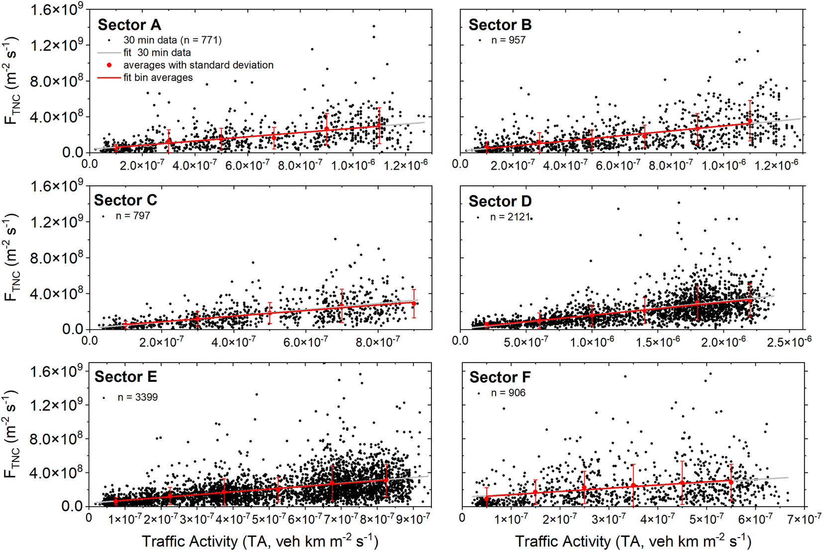 | ||
| Fig. 3 TNC fluxes (FTNC) as function of traffic activity (TA) for wind direction sectors A–F. Regressions fits (eqn (5)) for the 30 min flux data is indicated by the grey line, whereas the fit to the binned average (red dot with standard deviation as error bars) is indicated by the red line. | ||
 of all six sectors is also specified. The analysis of variance test (ANOVA) indicated that the regression slopes in all sectors were significantly different from zero (at the p = 0.05 level) and population means of particle fluxes and traffic activity were significantly different (Mann–Whitney test, p = 0.05)
| Sector | EFmf (veh−1 km−1) | F 0 (m−2 s−1) | R 2 | |
|---|---|---|---|---|
| A | All data | 2.35 × 10¹⁴ | 3.85 × 10⁷ | 0.25 |
| Bin average | 2.36 × 10¹⁴ | 3.61 × 10⁷ | 0.95 | |
| B | All data | 2.78 × 10¹⁴ | 1.90 × 10⁷ | 0.32 |
| Bin average | 2.81 × 10¹⁴ | 1.92 × 10⁷ | 0.96 | |
| C | All data | 3.46 × 10¹⁴ | 1.35 × 10⁷ | 0.32 |
| Bin average | 3.09 × 10¹⁴ | 2.63 × 10⁷ | 0.98 | |
| D | All data | 1.54 × 10¹⁴ | 0.75 × 10⁷ | 0.29 |
| Bin average | 1.45 × 10¹⁴ | 1.56 × 10⁷ | 0.99 | |
| E | All data | 3.36 × 10¹⁴ | 4.02 × 10⁷ | 0.22 |
| Bin average | 3.28 × 10¹⁴ | 4.20 × 10⁷ | 0.99 | |
| F | All data | 3.47 × 10¹⁴ | 11.0 × 10⁷ | 0.08 |
| Bin average | 3.80 × 10¹⁴ | 10.20 × 10⁷ | 0.89 | |
| Average (A–F) | All data | 2.83 × 10¹⁴ | 3.81 × 10⁷ | 0.25 |
| Bin average | 2.80 × 10¹⁴ | 4.02 × 10⁷ | 0.96 |
With exception of sector F, the binned values of F0 vary between 0.75 × 10⁷ to 4.02 × 10⁷ m−2 s−1, which corresponds to 6.3–33.8% of the 3 year average total particle number flux at this site, i.e. FTNC = 1.19 × 10⁸ m−2 s−1 (cf.20). The averaged TNC emission factor for sectors A–F resulted in 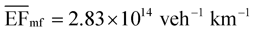 (±standard deviation of 0.71 × 10¹⁴ veh−1 km−1) for the 3 year period, whereas the average F0 was 3.81 (±3.4) × 107 m−2 s−1 (i.e. 32% of 3 year average TNC flux). Since traffic was found to be the main source of ultrafine particles at this site,20 a (minor) relative share of 6.3–33.8% of particles from other sources than traffic in the different sectors seems plausible. However, the F0 value of 11.0 × 10⁷ m−2 s−1 in sector F is distinctly larger than in the other sectors and nearly in the same order as the 3 year average particle number flux. The reason for the deviation from the other sectors is not yet clear, but might be related to a larger (unknown) particle emission source.
3.2 Evaluation of derived EFmf
In order to evaluate the robustness of the derived emission factors EFmf, we applied the method of linear regression (cf. Section 2.5) to each of the 16 sectors despite the amount of traffic activity (Fig. 4). While was higher by a factor of 2.7 in sectors A–F in comparison to the other sectors, the average F0 values were similar in sectors A–F and the other sectors (factor 1.2). This indicates similar sources of non-traffic particle emission in the 16 wind direction sectors, but higher and more immediate traffic influence in sectors A–F. Thus, the choice of sectors A–F for calculating traffic-related particle emission factors seems reasonable.
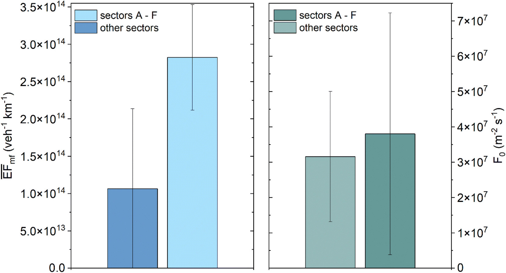 | ||
Fig. 4 (a) Average particle emission factors  and (b) average F0 (standard deviations are shown by error bars) for TNC in sectors A–F and the other sectors. Please note the different y-axis scaling. and (b) average F0 (standard deviations are shown by error bars) for TNC in sectors A–F and the other sectors. Please note the different y-axis scaling. | ||
3.3 Size-resolved analysis and inter-annual variation
The observation of size-resolved particle fluxes at our study site allows for the determination of emission factors for particles in different size ranges, e.g. the three modes NUC, AIT, and ACC. Most particles emitted by road traffic in the different sectors were in the nucleation mode, followed by particles in the Aitken mode (Fig. 5). The averaged emission factors for sectors A–F were 1.99 (±0.61) × 1014 veh−1 km−1 for NUC, 0.81 (±0.20) × 1014 veh−1 km−1 for AIT particles, and 0.09 (±0.02) × 1014 veh−1 km−1 for ACC mode particles. Thus, the amount of emitted UFP (as the sum of NUC and AIT modes) makes a fraction of 97% of total particles in the size range 10 nm < Dp < 200 nm. The fraction of particle emission in NUC mode is 69% of TNC. The differences between the sectors A–F with highest emission factors in sector C and F and lowest in D (cf.Fig. 3) are also evident for UFP and particle mode emissions (Fig. 5).
 | ||
| Fig. 5 Size-resolved average particle emission factors for road traffic in sectors A–F calculated from annual estimates. The standard deviation is depicted by error bars. | ||
The emission factors were characterised by inter-annual variation between the three observation years, e.g. the TNC emission factor decreased by about 17% from the first to the second year and increased by about 9% from the second to the third year (Fig. 6).
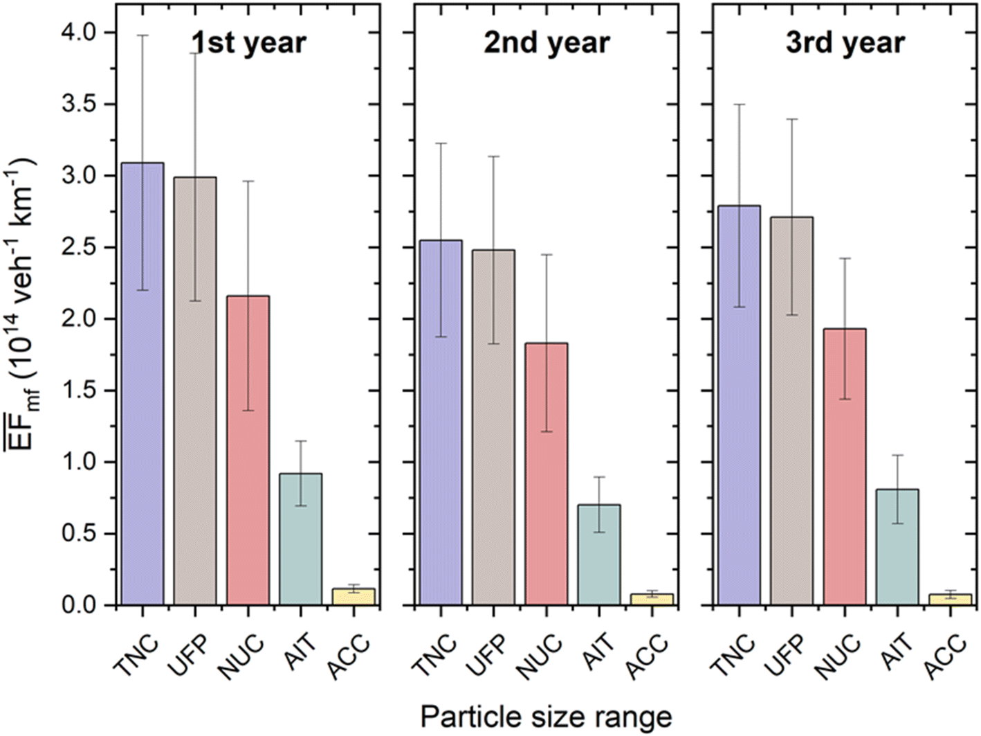 | ||
Fig. 6 Size-resolved average particle emission factors ( with standard deviation) for road traffic in sectors A–F for the three individual measurement years from April 2017 until March 2018 (1st year), April 2018 until March 2019 (2nd year), and April 2019 until March 2020 (3rd year). with standard deviation) for road traffic in sectors A–F for the three individual measurement years from April 2017 until March 2018 (1st year), April 2018 until March 2019 (2nd year), and April 2019 until March 2020 (3rd year). | ||
The coefficient of variation, which is defined as the quotient of the standard deviation and the arithmetic average across sectors A–F, is 26% for TNC. Thus, inter-annual differences of  are lower than the coefficient of variation across wind direction sectors indicating that robust temporal trends cannot be derived from the present data. The inter-annual variation of UFP, NUC, AIT, and ACC particle emission factors were in a similar range as the TNC variation with 26% for UFP, 26% for NUC, 29% for AIT, and 34% for ACC.
3.4 Particle emission factors for light-duty and heavy-duty vehicles
To analyse vehicle type-specific particle emission factors, i.e. emission factors for LDVs and HDVs, sector-wise multiple linear regression was performed using specific traffic data for LDVs and HDVs. It is evident that HDVs emit significantly more particles than LDVs with the ratios of the emission factors for HDV and LDVs varying between 9.5 < EFHDV/EFLDV < 15.3 (Fig. 7 and Table 2). The proportion of particle emission in NUC and AIT distinctly differs for LDVs and HDVs. The LDV fleet in Berlin emitted about three quarters of total particles in the NUC mode (i.e. 72% of total particles), followed by 25% in the AIT mode. The HDV fleet also dominantly emitted in the NUC mode, however, with 63% emission in the NUC mode the relative share was lower in comparison to the LDV fleet. The HDV fleet emitted 33% of total particles in the AIT mode.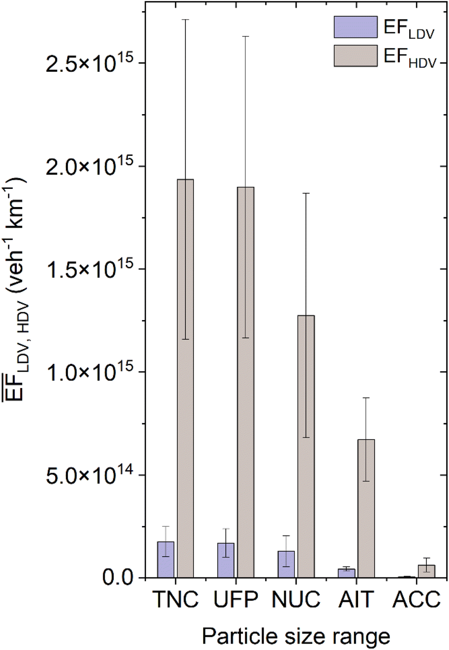 | ||
| Fig. 7 Size-resolved average particle emission factors (with standard deviation) for light-duty vehicles (EFLDV) and heavy-duty vehicles (EFHDV) for road traffic in sectors A–F. | ||
 from linear regression, and light-duty
  and heavy-duty vehicles
  from multiple linear regression. F0 is representing the particle emission flux from other sources (excluding vehicular traffic). The leftmost F0 specifies the intercept from the linear regression, whereas the other F0 gives the intercept from the multiple linear regression.
  quantifies the ratio of both emission factors. All values are derived from regression analysis for sectors A–F. Please note the different units
| Size | Linear regression | Multiple linear regression | ||||||
|---|---|---|---|---|---|---|---|---|
|
|
F 0 (107 m−2 s−1) | R 2 |
|
|
|
F 0 (107 m−2 s−1) | R 2 | |
| TNC | 2.83 (±0.77) | 3.81 (±3.42) | 0.25 | 1.77 (±0.73) | 19.35 (±7.76) | 10.9 | 3.66 (±3.50) | 0.27 |
| UFP | 2.74 (±0.75) | 3.71 (±3.45) | 0.25 | 1.69 (±0.69) | 18.98 (±7.32) | 11.2 | 3.57 (±3.53) | 0.27 |
| NUC | 1.99 (±0.67) | 2.40 (±2.61) | 0.22 | 1.30 (±0.75) | 12.74 (±5.93) | 9.8 | 2.31 (±2.66) | 0.25 |
| AIT | 0.82 (±0.22) | 1.79 (±0.81) | 0.19 | 0.44 (±0.11) | 6.72 (±2.01) | 15.3 | 1.75 (±0.84) | 0.21 |
| ACC | 0.09 (±0.02) | 0.35 (±0.06) | 0.15 | 0.06 (±0.02) | 0.62 (±0.33) | 10.3 | 0.34 (±0.06) | 0.17 |


Although the multiple linear regression models to determine EFLDV and EFHDV for the sectors A–F were statistically significant at the p = 0.05 level it has to be noted that the predictor variables LDV and HDV were correlated with r ≈ 0.8. Predictor variables with correlation coefficients of r > 0.7 point to collinearity which confines the understanding of the exact relationship between the predictors and response variables but does not impact model predictions (e.g.32). However, there should be some caution applied when transferring the present MLR estimates to other study sites, especially with different compositions of the traffic fleet such as different fractions of HDV.
4. Discussion
4.1 Comparison to literature estimates
In the past two decades, particle emission factors for road vehicles have been derived using different methods, e.g. on-road measurements, dynamometer measurements, NOx tracer method, and turbulent flux measurements applying the eddy covariance technique (cf.Table 3 for an overview). Generally, EFmf is influenced by multiple factors, such as the observed particle size range, fuel and vehicle type, driving patterns, topography, driving behaviour or vehicle age (e.g.18). Consequently, the determined emission factors span a wide range, with median or average values for mixed vehicle fleets varying from 0.2–14.6 × 10¹⁴ veh−1 km−1 (Table 3). The present EFmf for TNC characterising the mixed vehicle fleet in the flux source area around our study site in Berlin varies from 1.5–3.5 × 10¹⁴ veh−1 km−1 for the different wind direction sectors A–F. This is clearly within the range of EFmf as reported by others (Table 3).| Location/study | Size range (nm) | Emission factors (1014 veh−1 km−1) | Fraction of HDV (%) | Method | ||
|---|---|---|---|---|---|---|
| EFmf | EFLDV | EFHDV | ||||
| a Uncertainty not specified. b % diesel in vehicle fleet. c Median ± Q (semiquartile). d Mean ± standard error. e 95% confidence interval. f Median ± standard error. g Mean (IQR). h Median ± median absolute deviation. i Daily mean (05:00–23:00). j Mean ± standard deviation. k Most realistic value (sector D). l Typical motorway traffic conditions. m Typical urban traffic conditions with most vehicles traveling in a stop-start mode between two traffic lights. | ||||||
| Copenhagen (Denmark)36 | 10–700 | 2.8 ± 0.5a | — | — | 6–8 | Roadside measurements with inverse modelling (street canyon) |
| Minnesota (Minneapolis, USA)35 | 8–300 | 0.9–2.7 | — | — | 9b | On-road measurements (motorway) |
| 3–1000 | 1.9–9.9 | |||||
| Brisbane (Australia)13 | 15–700 | 1.11 ± 0.90c (Tora St)l | — | — | 6 | On-road measurements with box model |
| 15–700 | 0.57 ± 0.28c (Ipswich Rd)m | — | — | 15 | ||
| Minnesota (Minneapolis, USA)39 | >3 | — | 6.2 ± 1.4d | 42.0 ± 6.0d | — | On-road measurements (motorway) |
| 8–300 | 0.34 ± 0.05d | 6.6 ± 1.0d | ||||
| Stockholm (Sweden)15 | >11 | 1.4 ± 0.2e | 0.3 ± 0.3e | 19.8 ± 4.0e | 6 | Eddy covariance (lin. regression with traffic activity) |
| Berlin (Germany)9 | 10–500 | 2.1 ± 0.2a | 0.24 ± 0.15a | 29.6 ± 3.5a | 6 | Roadside measurements with inverse modelling (motorway) |
| 10–50 | 1.3 ± 0.2a | |||||
| Helsinki (Finland)42 | 6–5000 | 3.0 ± 1.1f | — | — | — | Eddy covariance (footprint estimation, traffic rate) |
| Copenhagen (Denmark)37 | 10–700 | 2.15 ± 0.05d (motorway) | 0.81 ± 0.07d (motorway) | 17.5 ± 0.68d (motorway) | 8 | NOx tracer method (motorway and urban street) |
| 1.87 ± 0.03d (urban street) | 1.01 ± 0.06d (urban street) | 22.06 ± 1.28d (urban street) | ||||
| Lecce (Italy)38 | 9–1000 | 2.9 (2.2–5.0)g | — | — | — | Eddy covariance (footprint estimation, traffic rate) |
| Boston (Massachusetts, USA)43 | 4–3000 | Southbound tunnel: 5.1 ± 2.3h | — | — | 2–5b | On-road measurements (motorway tunnel) |
| Northbound tunnel: 1.4 ± 0.42h | — | — | 1–3b | |||
| Meckenheim (Germany)40 | 14–750 | 3.7 | 2.1 | 11.8 | 18 | NOx tracer method (motorway) |
| 14–50 | 3.1 | 1.6 | 10.9 | |||
| 14–100 | 3.5 | 1.9 | 11.4 | |||
| 50–200 | 0.6 | 0.5 | 0.7 | |||
| Londrina (Brazil)18 | >10 | 14.6i | 9.25 ± 1.13d | 37.28 ± 5.79d | 13 | Roadside measurements with inverse modelling (street canyon) |
| Lecce (Italy)34 | 9–3000 | 2.2 ± 0.62d | — | — | — | Eddy covariance (footprint estimation, traffic rate) |
| Mumbai (India)44 | >10 | 0.21 ± 0.05j | — | — | 2 | On-road measurements (motorway tunnel) |
| Berlin (Germany)/this study | 10–200 | 2.83 ± 0.70j | 1.77 ± 0.73j | 19.36 ± 7.77j | 6 | Eddy covariance (lin. regression with traffic activity) |
| (1.54)k | (1.01)k | (10.37)k | ||||
| 10–100 | 2.74 ± 0.69j | 1.69 ± 0.69j | 19.00 ± 7.33j | |||
| (1.49)k | (0.97)k | (10.30)k | ||||
| 10–30 | 1.99 ± 0.61j | 1.30 ± 0.75j | 12.74 ± 5.93j | |||
| (1.00)k | (0.61)k | (7.70)k | ||||
| 30–100 | 0.81 ± 0.20j | 0.44 ± 0.11j | 6.72 ± 2.02j | |||
| (0.48)k | (0.36)k | (2.51)k | ||||
| 100–200 | 0.09 ± 0.02j | 0.06 ± 0.02j | 0.63 ± 0.33j | |||
| (0.05)k | (0.05)k | (0.09)k | ||||
Due to the considerable emission of UFPs from road traffic,9,20,33,34 the lower cut-off of particle sizing or counting instruments may explain higher emission factors in case of a lower cut-off size, e.g. EFmf of 0.9–2.7 × 10¹⁴ veh−1 km−1 with cut-off Dp = 8 nm vs. EFmf of 1.9–9.9 × 10¹⁴ veh−1 km−1 with cut-off Dp = 3 nm (35; Table 3). Studies having a similar lower diameter cut-off (e.g. 9–11 nm) and a similar proportion of HDV in the mixed vehicle fleet compared to our site in Berlin, reported emission factors between 1.4 × 10¹⁴ veh−1 km−1 and 2.9 × 10¹⁴ veh−1 km−1.9,15,34,36–38 The sector-averaged TNC emission factor of  as derived from the present data is exactly within this range. However, in contrast to the study by Birmili et al.9 who estimated EFmf by an inverse modelling approach close to the motorway A100 in Berlin (mean traffic driving speed of 80 km h−1), the present
  for TNC is larger by about 0.7 × 10¹⁴ veh−1 km−1. This is somewhat surprising as a lower emission factor may have been expected with respect to the assumption that a mixed urban vehicle fleet modernises in certain time intervals and that a higher share of vehicles with cleaner emission technology should be present nowadays in comparison to the Birmili et al.9 study conducted about 14 years ago. However, it is difficult to compare both estimates as the one was conducted close to a motorway, over a short summer period of 10 weeks, and was measured over a larger diameter size range (i.e. 10 < Dp < 500 nm), whereas the present study observed more typical urban driving patterns which may have been influenced by a higher share of congested traffic situations, especially during rush-hour traffic.
As stated in the introduction, our study aims to quantify a ‘typical’ mixed-fleet road traffic emission factor which is representative for urban Berlin. Hence, we focussed on the quantification of an average weekday situation with commuting traffic and excluded periods with ‘non-typical’ traffic situations such as weekends or holidays. Stratification of the data-set into specific situation such as seasonal variation (winter vs. summer particle EFs), or weekend vs. weekday comparison will result in smaller groups of data being subject to the regression approach (cf.eqn (5)). This would likely increase the variance in the data resulting in more uncertain particle EFs. The analysis of the potential of the regression method for estimation of more specific particle EFs, however, would be an interesting subject for future research. The derived emission factors for light and heavy duty vehicles are within the literature range of 0.24–9.25 × 10¹⁴ veh−1 km−1 for EFLDV and 6.6–42.0 × 10¹⁴ veh−1 km−1 for EFHDV (cf.Table 2). However, most other studies with a similar lower cut-off (i.e. Dp of 8–11 nm) report EFLDV that are smaller by a factor of 5–7 compared to this study. The results of EFLDV for Londrina, Brazil with 9.25 (±1.13) × 1014 veh−1 km−1 (ref. 18) and for Minnesota, USA with 6.2 (±1.4) × 1014 veh−1 km−1 are higher than at the Berlin site.39 Our calculated EFHDV, however, is in the range of estimates as reported by others and very close to figures reported for Stockholm, Sweden15 and Copenhagen, Denmark.37
The finding that size-resolved particle emission factors for road traffic tend to increase with smaller particle diameters, is in agreement with our observations at the Berlin site as the largest particle emission factors were evident for the NUC mode, followed by the AIT mode (e.g.34,40).
4.2 Limitations of the study
When determining particle emission factors using linear and multiple linear regression of traffic activity and eddy covariance particle flux data (cf.15), the quality of the results depends on relationship between both quantities in the flux source area, i.e. the slope of the regression equation. Hence, the certainty of the emission factor should improve with the quality of the traffic data and the particle fluxes. In the present study, traffic activity was estimated using wind direction sectors covering an area of 2 km radius. Due to this rather simplified approach, an under- or overestimation of traffic activity cannot be ruled out, as roads in the sector have different traffic intensity, i.e. major and minor roads, and the flux source area is not homogeneously distributed across the 2 km study area.20 This may result in a ‘mismatch’ between the variation in particle fluxes as driven from the flux source area vs. traffic intensity as estimated from the 2 km sector. Consequently, this will influence the certainty in the particle EF quantification.An underestimation of traffic activity in a sector would lead to an increased slope of the regression line and thus to an increased emission factor. An overestimation, on the other hand, would lead to a lower emission factor. Due to the nearby “Straβe des 17. Juni” to the north of the measurement station, which more significantly contributes to the particle flux than more distant areas within the 2 km radius, there may have been an underestimation of traffic activity in some sectors resulting in a slight overestimation of EFmf. In sector D, which shows the highest amount of streets in the land-use of the flux source area (53%, cf.20) and is associated with the highest traffic activity of the six selected sectors, the estimated traffic activity therefore might be more certain than in the other sectors. More sophisticated flux source area modelling applying a source area-weighted estimation of traffic intensity may decrease uncertainty in the traffic estimation and consequently in the particle EF.41
Flux source area-weighted modelling may also help improving annual trend estimation of particle EFs as in the current state the annual differences are lower than the variation across the sectors A–F, i.e. the coefficient of variation (cf. Section 3.3). This implies that robust temporal trends cannot be derived from the present data. Temporal variation of particle fluxes, however, such as differences between the different observation years, might be associated with spatial shifts of the peak contribution location of the flux source area during the observation years. In a previous study we documented that in the second year, for instance, the average wind direction and also the peak flux source area shifted towards areas with lower traffic intensity, i.e. north–westerly directions.20
The transition of the mixed traffic fleet towards a higher fraction of low-emission standards or electric vehicles poses further variation of particle fluxes, as the proportion of electric vehicles in Berlin increased by a factor of 3 in the time period from 2017 to 2020.20 However, the estimation of this influence would require more specific data such as the share of electric vehicles at hourly resolution, which were not available for the present analysis.
5 Summary and conclusions
Size-resolved particle emission factors were derived from 3 years of eddy-covariance particle number flux observations in Berlin, Germany. The averaged emission factor of for TNC is in the range of road traffic emission factors as reported in literature. The results indicate strongest particle emission from the mixed fleet to occur in the nucleation mode, i.e. 69% of total mixed fleet particle emission. The analysis for LDV and HDV indicated significantly higher EFHDV than EFLDV with, for instance, ratios of EFHDV/EFLDV = 11.2 for UFP, and 9.8 for NUC. However, some uncertainty in the calculation of emission factors arises from the estimation of sector-wise traffic activity, as this influences the slope of the regression equations to quantify particle emission factors. The study demonstrates the method of linear (multiple) regression between eddy covariance fluxes and traffic data to be a promising tool to derive particle emission factors for a vehicle fleet in the source area of eddy-covariance flux measurements. The method relies on the quality of both, the particle flux data and the traffic activity in the flux source area. The latter was estimated by a simplified approach in the present study which leaves some room for future improvement.
Generally, eddy covariance particle flux measurements prove a powerful tool to quantify (size-resolved) particle emission factors. Long-term measurements may help to study annual variation and trends in emission factors and may help to monitor the effects of the modernisation of the traffic fleet or traffic reduction measures on urban air quality.
6 Appendix
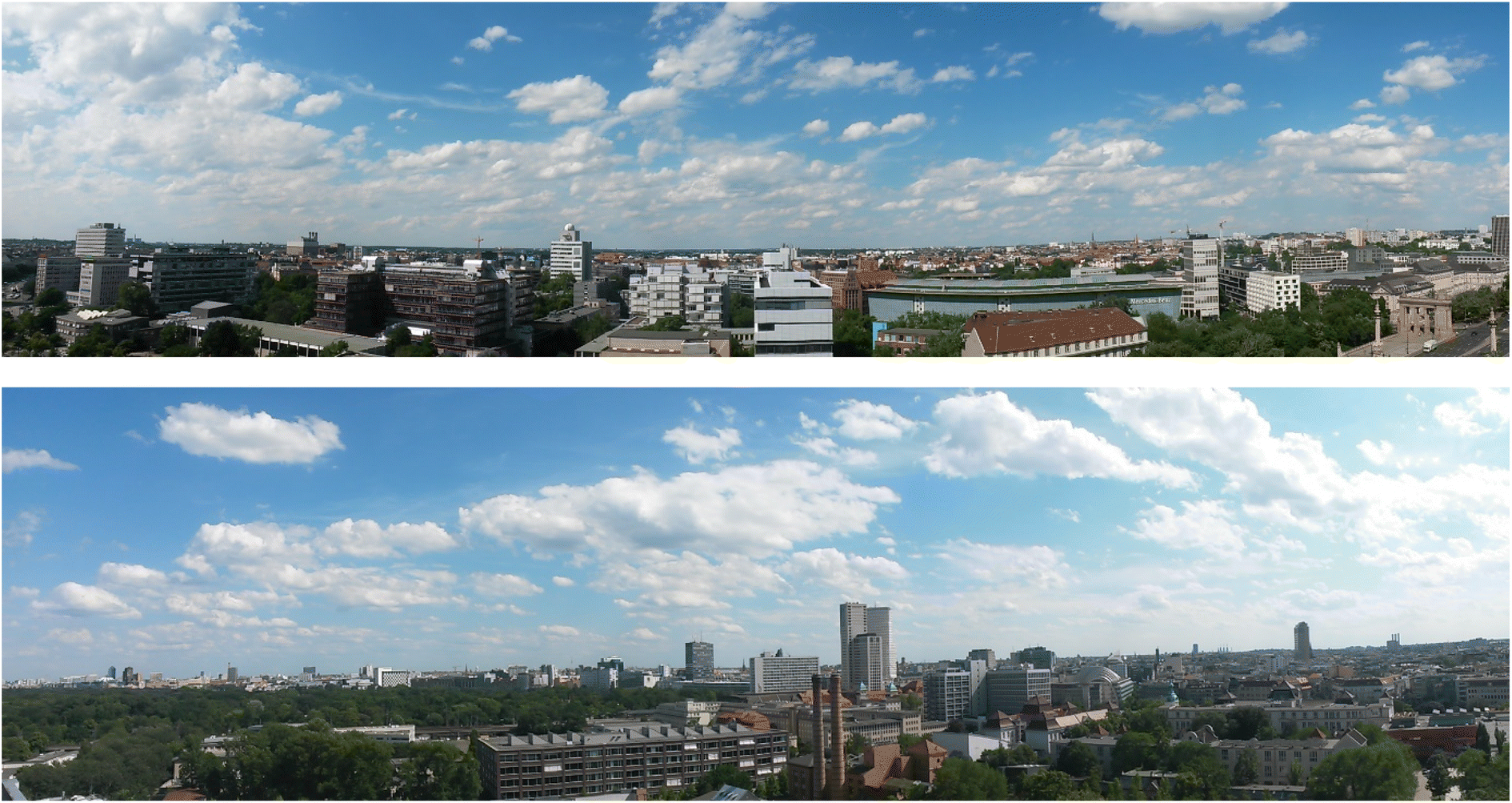 | ||
| Fig. 8 Panoramic views of the site surroundings taken from rooftop of Technische Universität Berlin. (Top) The picture shows the areas northeast and west (270°–80°) of the site, (bottom) the area east and south of the site (90°–260°, pictures: Stephan Weber). | ||
 | ||
| Fig. 9 Average (a) emission and (b) deposition particle number fluxes in the different wind sectors for nucleation (FNUC), Aitken (FAIT), and accumulation (FACC) mode fluxes (Straaten and Weber, 2021).20 | ||
Conflicts of interest
There are no conflicts to declare.Acknowledgements
We would like to thank Daniel Weber from Senate Department for the Environment, Urban Mobility, Consumer Protection and Climate Action of the Berlin city administration for providing hourly traffic data from 22 traffic counting stations in the study area. We further thank our project partners (Dieter Scherer and Fred Meier) of the Chair of Climatology, Institute of Ecology, Technische Universität Berlin for the opportunity to conduct long-term particle flux measurements at their urban climate observatory. Another thank goes to Hagen Mittendorf of Technische Universität Braunschweig for supporting the flux site maintenance. This study was supported by the German Federal Ministry of Education and Research (BMBF; grant nos. FKZ 01 LP 1602 D – Urban Climate Under Change, Module 3DO – and FKZ 01 LP 1912 D – Urban Climate Under Change, phase II, Module 3DO+M).References
- P. Kumar, L. Morawska, W. Birmili, P. Paasonen, M. Hu, M. Kulmala, R. M. Harrison, L. Norford and R. Britter, Ultrafine particles in cities, Environ. Int., 2014, 66, 1–10 CrossRef CAS PubMed.
- C. von Bismarck-Osten, W. Birmili, M. Ketzel, A. Massling, T. Petäjä and S. Weber, Characterization of parameters influencing the spatio-temporal variability of urban aerosol particle number size distributions in four European cities, Atmos. Environ., 2013, 77, 415–429 CrossRef CAS.
- M. C. Simon, N. Hudda, E. N. Naumova, J. I. Levy, D. Brugge and J. L. Durant, Comparisons of traffic-related ultrafine particle number concentrations measured in two urban areas by central, residential, and mobile monitoring, Atmos. Environ., 2017, 169, 113–127 CrossRef CAS PubMed.
- I. Rivas, D. C. S. Beddows, F. Amato, D. C. Green, L. Järvi, C. Hueglin, C. Reche, H. Timonen, G. W. Fuller, J. V. Niemi, N. Pérez, M. Aurela, P. K. Hopke, A. Alastuey, M. Kulmala, R. M. Harrison, X. Querol and F. J. Kelly, Source apportionment of particle number size distribution in urban background and traffic stations in four European cities, Environ. Int., 2020, 135, 105345 CrossRef CAS PubMed.
- S. Ohlwein, R. Kappeler, M. Kutlar Joss, N. Künzli and B. Hoffmann, Health effects of ultrafine particles: a systematic literature review update of epidemiological evidence, Int. J. Public Health, 2019, 64(4), 547–559 CrossRef PubMed.
- H.-S. Kwon, M. H. Ryu and C. Carlsten, Ultrafine particles: unique physicochemical properties relevant to health and disease, Exp. Mol. Med., 2020, 52(3), 318–328, DOI:10.1038/s12276-020-0405-1.
- European Commission, Proposal for a Directive of the European Parliament and of the Council on Ambient Air Quality and Cleaner Air for Europe, 2022, 542 final/2, p. 75 Search PubMed.
- L. Morawska, Z. Ristovski, E. R. Jayaratne, D. U. Keogh and X. Ling, Ambient nano and ultrafine particles from motor vehicle emissions: Characteristics, ambient processing and implications on human exposure, Atmos. Environ., 2008, 42(35), 8113–8138 CrossRef CAS.
- W. Birmili, B. Alaviippola, D. Hinneburg, O. Knoth, T. Tuch, J. Borken-Kleefeld and A. Schacht, Dispersion of traffic-related exhaust particles near the Berlin urban motorway – estimation of fleet emission factors, Atmos. Chem. Phys., 2009, 9(7), 2355–2374, DOI:10.5194/acp-9-2355-2009.
- P. Brimblecombe, T. Townsend, C. F. Lau, A. Rakowska, T. L. Chan, G. Močnik and Z. Ning, Through-tunnel estimates of vehicle fleet emission factors, Atmos. Environ., 2015, 123, 180–189 CrossRef CAS.
- Y. Fujitani, K. Takahashi, A. Fushimi, S. Hasegawa, Y. Kondo, K. Tanabe and S. Kobayashi, Particle number emission factors from diesel trucks at a traffic intersection: Long-term trend and relation to particle mass-based emission regulation, Atmos. Environ.: X, 2020, 5, 100055 CAS.
- L. Gerling and S. Weber, Mobile measurements of atmospheric pollutant concentrations in the pollutant plume of BER airport, Atmos. Environ., 2023, 304, 119770 CrossRef CAS.
- L. Morawska, M. Jamriska, S. Thomas, L. Ferreira, K. Mengersen, D. Wraith and F. McGregor, Quantification of particle number emission factors for motor vehicles from on-road measurements, Environ. Sci. Technol., 2005, 39(23), 9130–9139, DOI:10.1021/es050069c.
- A. M. Jones and R. M. Harrison, Estimation of the emission factors of particle number and mass fractions from traffic at a site where mean vehicle speeds vary over short distances, Atmos. Environ., 2006, 40(37), 7125–7137 CrossRef CAS.
- E. M. Mårtensson, E. D. Nilsson, G. Buzorius and C. Johansson, Eddy covariance measurements and parameterisation of traffic related particle emissions in an urban environment, Atmos. Chem. Phys., 2006, 6, 769–785, DOI:10.5194/acp-6-769-2006.
- S. Janhäll, P. Molnar and M. Hallquist, Traffic emission factors of ultrafine particles: effects from ambient air, J. Environ. Monit., 2012, 14(9), 2488–2496 RSC.
- V. Franco, M. Kousoulidou, M. Muntean, L. Ntziachristos, S. Hausberger and P. Dilara, Road vehicle emission factors development: A review, Atmos. Environ., 2013, 70, 84–97 CrossRef CAS.
- P. Krecl, A. C. Targino, T. P. Landi and M. Ketzel, Determination of black carbon, PM2.5, particle number and NOx emission factors from roadside measurements and their implications for emission inventory development, Atmos. Environ., 2018, 186, 229–240, DOI:10.1016/j.atmosenv.2018.05.042.
- L. Järvi, C. S. B. Grimmond and A. Christen, The Surface Urban Energy and Water Balance Scheme (SUEWS): Evaluation in Los Angeles and Vancouver, J. Hydrol., 2011, 411(3–4), 219–237, DOI:10.1016/j.jhydrol.2011.10.001.
- A. Straaten and S. Weber, Measurement report. Three years of size-resolved eddy-covariance particle number flux measurements in an urban environment, Atmos. Chem. Phys., 2021, 21(24), 18707–18726, DOI:10.5194/acp-2021-625.
- D. Scherer, F. Ament, S. Emeis, U. Fehrenbach, B. Leitl, K. Scherber, C. Schneider and U. Vogt, Three-Dimensional Observation of Atmospheric Processes in Cities, Metz, 2019, 28, 121–138, DOI:10.1127/metz/2019/0911.
- J. A. Quanz, Impact of spatial heterogeneity on energy exchange in an urban environment in Berlin, Germany, Master thesis, Technische Universität Berlin, 2018, p. 85.
- Geoportal Berlin, Biotope types, license “dl-de/by-2-0”, 2014. Available at: https://www.berlin.de/umweltatlas/en/biotopes/biotope-types/continually-updated/summary/, accessed July 2023; Traffic volumes 2019, license "dl-de/by-2-0", available at: https://www.berlin.de/umweltatlas/en/traffic-noise/traffic-volumes/2019/summary/, accessed July 2023; ALKIS Berlin Building types, license “dl-de/by-2-0”, available at: https://daten.berlin.de/datensaetze/alkis-berlin-geb%C3%A4ude-wfs, accessed July 2023.
- A. Meyer-Kornblum, L. Gerling and S. Weber, Gap-filling fast electrical mobility spectrometer measurements of particle number size distributions for eddy covariance application, Aerosol Air Qual. Res., 2019, 19(12), 2721–2731, DOI:10.4209/aaqr.2019.06.0291.
- W. C. Hinds, Aerosol Technology, Properties, Behavior, and Measurement of Airborne Particles, Wiley, New York, 2nd edn, 1999 Search PubMed.
- D. Vickers and L. Mahrt, Quality control and flux sampling problems for tower and aircraft data, J. Atmos. Ocean. Technol., 1997, 14(3), 512–526, DOI:10.1175/1520-0426(1997)014<0512:QCAFSP>2.0.CO;2.
- J. B. Moncrieff, J. M. Massheder, H. de Bruin, J. Elbers, T. Friborg, B. Heusinkveld, P. Kabat, S. Scott, H. Soegaard and A. Verhoef, A system to measure surface fluxes of momentum, sensible heat, water vapour and carbon dioxide, J. Hydrol., 1997, 188–189, 589–611 CrossRef CAS.
- J. Moncrieff, R. Clement, J. Finnigan and T. Meyers, Averaging, detrending, and filtering of eddy covariance time series, in Handbook of Micrometeorology, ed. Lee X., Massman W. and Law B., Springer, Dordrecht, Atmos. Ocean. Sci. Lib. 29, 2004 Search PubMed.
- T. W. Horst, A simple formula for attenuation of eddy fluxes measured with first-order response scalar sensors, Bound.-Layer Meteorol., 1997, 82(2), 219–233, DOI:10.1023/A:1000229130034.
- T. Foken, M. Göockede, M. Mauder, L. Mahrt, B. Amiro and W. Munger, in Post-Field Data Quality Control (Handbook of Micrometeorology), ed. Lee X., Massman W. and Law B., Springer, Dordrecht, Atmos. Ocean. Sci. Lib. 29, 2004 Search PubMed.
- L. Gerling and S. Weber, Atmospheric transformation of urban particle number size distributions during the transport along street canyons as quantified by an aerosol sectional model, Atmos. Pollut. Res., 2022, 13(2), 101296 CrossRef.
- C. F. Dormann, J. Elith, S. Bacher, C. Buchmann, G. Carl, G. Carré, J. Marquéz, B. Gruber, B. Lafourcade, P. J. Leitão, T. Münkemüller, C. McClean, P. E. Osborne, B. Reineking, B. Schröder, A. K. Skidmore, D. Zurell and S. Lautenbach, Collinearity: a review of methods to deal with it and a simulation study evaluating their performance, Ecography, 2013, 36(1), 27–46 CrossRef.
- M. J. Deventer, L. von der Heyden, C. Lamprecht, M. Graus, T. Karl and A. Held, Aerosol particles during the Innsbruck Air Quality Study (INNAQS): Fluxes of nucleation to accumulation mode particles in relation to selective urban tracers, Atmos. Environ., 2018, 190, 376–388, DOI:10.1016/j.atmosenv.2018.04.043.
- M. Conte and D. Contini, Size-resolved particle emission factors of vehicular traffic derived from urban eddy covariance, Environ. Pollut., 2019, 251, 830–838, DOI:10.1016/j.envpol.2019.05.029.
- D. W. Kittelson, W. F. Watts and J. P. Johnson, Nanoparticle emissions on Minnesota highways, Atmos. Environ., 2004, 38, 9–19, DOI:10.1016/j.atmosenv.2003.09.037.
- M. Ketzel, P. Wåhlin, R. Berkowicz and F. Palmgren, Particle and trace gas emission factors under urban driving conditions in Copenhagen based on street and roof-level observations, Atmos. Environ., 2003, 37, 2735–2749, DOI:10.1016/S1352-2310(03)00245-0.
- F. Wang, M. Ketzel, T. Ellermann, P. Wahlin, S. S. Jensen, D. Fang and A. Massling, Particle number, particle mass and NOx emission factors at a highway and an urban street in Copenhagen, Atmos. Chem. Phys., 2010, 10, 2745–2764, DOI:10.5194/acp-10-2745-2010.
- D. Contini, A. Donateo, C. Elefante and F. M. Grasso, Analysis of particles and carbon dioxide concentrations and fluxes in an urban area, Atmos. Environ., 2019, 46, 25–35, DOI:10.1016/j.atmosenv.2022.10.039.
- J. P. Johnson, D. B. Kittelson and W. F. Watts, Source apportionment of diesel and spark ignition exhaust aerosol using on-road data from the Minneapolis metropolitan area, Atmos. Environ., 2005, 39, 2111–2121, DOI:10.1016/j.atmosenv.2004.12.018.
- C. Nickel, H. Kaminski, B. Hellack, U. Quass, A. John, O. Klemm and T. A. J. Kuhlbusch, Size resolved particle number emission factors of motorway traffic differentiated between heavy and light duty vehicles, Aerosol Air Qual. Res., 2013, 13(2), 450–461, DOI:10.4209/aaqr.2012.07.0187.
- H. Chu, X. Luo, Z. Ouyang, W. S. Chan, S. Dengel, S. C. Biraud, M. S. Torn, S. Metzger, J. Kumar, M. A. Arain, T. J. Arkebauer, D. Baldocchi, C. Bernacchi, D. Billesbach, T. A. Black, P. D. Blanken, G. Bohrer, R. Bracho, S. Brown, N. A. Brunsell, J. Chen, X. Chen, K. Clark, A. R. Desai, T. Duman, D. Durden, S. Fares, I. Forbrich, J. A. Gamon, C. M. Gough, T. Griffis, M. Helbig, D. Hollinger, E. Humphreys, H. Ikawa, H. Iwata, Y. Ju, J. F. Knowles, S. H. Knox, H. Kobayashi, T. Kolb, B. Law, X. Lee, M. Litvak, H. Liu, J. W. Munger, A. Noormets, K. Novick, S. F. Oberbauer, W. Oechel, P. Oikawa, S. A. Papuga, E. Pendall, P. Prajapati, J. Prueger, W. L. Quinton, A. D. Richardson, E. S. Russell, R. L. Scott, G. Starr, R. Staebler, P. C. Stoy, E. Stuart-Haëntjens, O. Sonnentag, R. C. Sullivan, A. Suyker, M. Ueyama, R. Vargas, J. D. Wood and D. Zona, Representativeness of Eddy-Covariance flux footprints for areas surrounding AmeriFlux sites, Agric. For. Meteorol., 2021, 301–302, 108350 CrossRef.
- L. Järvi, Ü. Rannik, I. Mammarella, A. Sogachev, P. P. Aalto, P. Keronen, E. Siivola, M. Kulmala and T. Vesala, Annual particle flux observations over a heterogeneous urban area, Atmos. Chem. Phys., 2009, 9(3), 13407–13437, DOI:10.5194/acpd-9-13407-2009.
- J. L. Perkins, L. T. Padró-Martínez and J. L. Durant, Particle number emission factors for an urban highway tunnel, Atmos. Environ., 2013, 74, 326–337, DOI:10.1016/j.atmosenv.2013.03.046.
- N. Raparthi, S. Debbarma and H. C. Phuleria, Development of real-world emission factors for on-road vehicles from motorway tunnel measurements, Atmos. Environ.: X, 2021, 10, 100113, DOI:10.1016/j.aeaoa.2021.100113.
| This journal is © The Royal Society of Chemistry 2023 |