A portable sensor for the determination of tree canopy air quality

Abstract

Using low-cost air quality sensors (PM_2.5, NO₂, CO), air pumps, and a Raspberry Pi computer, we constructed a system by which air quality in tree canopies could be interrogated and quantified. The system involves pumping air into a sensor-containing box alternatively from tree canopy air and ambient air; repeating often enough to document if there are concentration differences between these two sources. By using the same set of sensors for air analysis from two sources, we eliminate issues such as sensor offset or drift and/or sensitivity to environmental conditions. True differences between tree canopy air and ambient air can be verified only after it has been established that the concentration difference between co-located inlet tubes is negligible. We've documented co-location results, described data summary protocol and as proof of concept, we show true differences in PM_2.5 (production) and CO (consumption) between ambient air and tree canopies on the University of Southern California's campus. In one tree tested, NO₂ between tree canopy and ambient air fluctuated as a function of day/night indicating periods of production and consumption. This system can be applied to document which tree species modify air quality, and how much, and can thus help urban forestry decision-makers when choosing tree planting under various environmental conditions.

---

Environmental significance

Urban air quality is a growing concern as it relates to human health and global change. A strategy for increasing the desirability and livability of urban settings has been to ‘green’ them, add trees. Yet the type of trees suitable for a given location might be different from those planted if tree uptake and emission of certain air constituents were documented and quantified. Our goal was to build low cost air quality sensors that could interrogate tree canopy air and compare it to ambient air so as to establish which tree is emitting or taking up how much particulate matter, CO and NO₂.

Introduction

The interactions between the biosphere and atmospheric chemistry are complicated and made more complex as anthropogenic compounds have been entering our atmosphere for the past few hundred years. Trees in general, and urban trees in particular are thought to be beneficial to air quality given some studies that show their uptake of airborne constituents considered harmful to human health.^1,2 Conversely, trees may contribute to worsened air quality given the particular species, the proximity to other reactants, increases in air temperature and other conditions that influence the interactions between air and trees.^3,4

Urban tree planting is often seen through a lens that focuses on the benefits of shade and cooling and the aesthetics of green space.⁵ Yet urban trees likely function quite differently than trees in a natural or native setting given the isolation of trees planted along roadways, their soil composition and water supply is very different than for trees growing naturally. Further, trees can impact air quality in urban settings by the physical dispersion or trapping of pollution plumes in addition to their capability of biochemical uptake and/or production. For these reasons we advocate studies of urban trees on a tree-by-tree response basis.

The kinetics of pollutant uptake by trees is not well known and thus the residence time of air in contact with the foliage of a tree, its canopy, must be another important variable regarding the importance of trees impacting air quality. Canopy air residence time is likely a function of the density of the canopy and the strength of air movement, i.e. wind speed and turbulence. As every tree will have a different canopy, exposure to wind and physiological state, every tree might behave differently in terms of modifying air chemistry. The objective of this work is not to quantify fluxes, although that would be most useful from a modeling perspective, rather it is to demonstrate a methodology whereby quantitative differences between tree species in terms of air quality impact can be determined.

Another key factor to consider in terms of a tree's air quality impact is the dynamic range of air constituent variability and how sensitive a sensor is to small changes against a larger background. In the Los Angeles, mid-city region where tree canopy air testing took place, the ranges in PM_2.5, CO and NO₂ are typically 0–50 μg m⁻³; 0.2–2 ppm; 0–0.50 ppm respectively. The lowest values represent times when marine air is well mixed into the city as this air has near zero concentrations of these constituents. Highest concentrations are found during overnight hours when the planetary boundary layer is lowest.⁶ These ranges represent measured values from January through August, 2022 obtained using a BEACO2N (https://beacon.berkeley.edu/about/) sensor located at the University of Southern California (USC) which was calibrated by co-locating it for 2 weeks next to South Coast Air Quality Management District (SCAQMD) sensors located in downtown Los Angeles (1630 N. Main Street). The tree canopy study took place on USC's campus.

We aim to address tree canopy air quality relative to the air that is not directly within the tree canopy. We are asking if these two air measurements are significantly different from each other, and if so, in what direction. We developed a sensor system that could make measurements over 24 hours because concentrations change considerably over the diurnal period as does the average wind speed. With a solar panel (not discussed here), the sensors can run continuously. We found that using two sensors, one located in a tree canopy and another outside the tree canopy was not the optimal experimental design because of inherent offsets and sensitivities of low-cost sensors to environmental conditions. Instead, we've designed and tested a method to interrogate air quality within a tree canopy and outside the tree canopy with a single set of sensors and an alternating pumping system.

Methodology

The premise of our design, illustrated in Fig. 1, is to alternate uptake of air from inside and then outside the tree canopy of interest while passing this air by sensors located in a sealed box. In this switching mode a constituent is always measured by the same sensor. Although using two sensor boxes, one in the tree canopy and one outside is a logical way to compare air quality between two locations, no two sensors will behave exactly the same and sensors will also be subject to sensitivity to differences in temperature and humidity between locations. Below we discuss the construction of our sensors and the pump switching design.

Fig. 1 Schematic of air quality sensor box configured to pump air through either a tube running up to a tree canopy (tube #1) or a tube sampling ambient air from outside the tree canopy (tube #2).

Sensor circuit board design

We started with a blank circuit board 8 × 12 cm onto which we hand-soldered and wired: NO₂, CO sensors (Alphasense); PM_2.5 (Plantower PMSA003I); Raspberry Pi Zero; Time, temperature and humidity sensor (Adafruit AHT20); LED screen (Adafruit I2Cpi); Analog to Digital converter (ADS 1115). A thorough discussion of the performance of the Alphasense and Plantower sensors can be found in Kim et al., 2018 (ref. 7) and Shusterman et al., 2019,⁸ and in Table 1 where we have summarized their output. The circuit board with sensors attached is pictured in Fig. 2A. A cell-phone rechargeable battery brick provides power to the circuit board and to two external pumps.

Table 1 Information about sensors and link to specifications sheet

Sensor	Make/model	Output	Response time
CO	Alphasense B4	∼280 mV @ 0 ppm	<90 s
		∼730 mV @ 1 ppm
https://www.alphasense.com/wp-content/uploads/2022/09/Alphasense_CO-B4_datasheet.pdf
NO2	Alphasense B43F	∼205 mV @ 0 ppm	<90 s
		∼240 mV @ 0.2 ppm
https://www.alphasense.com/wp-content/uploads/2022/09/Alphasense_NO2-B43F_datasheet.pdf
PM2.5	Plantower PMSA003	Output in μg m^−3	<10 s
https://plantower.com/en/products_33/77.html

---

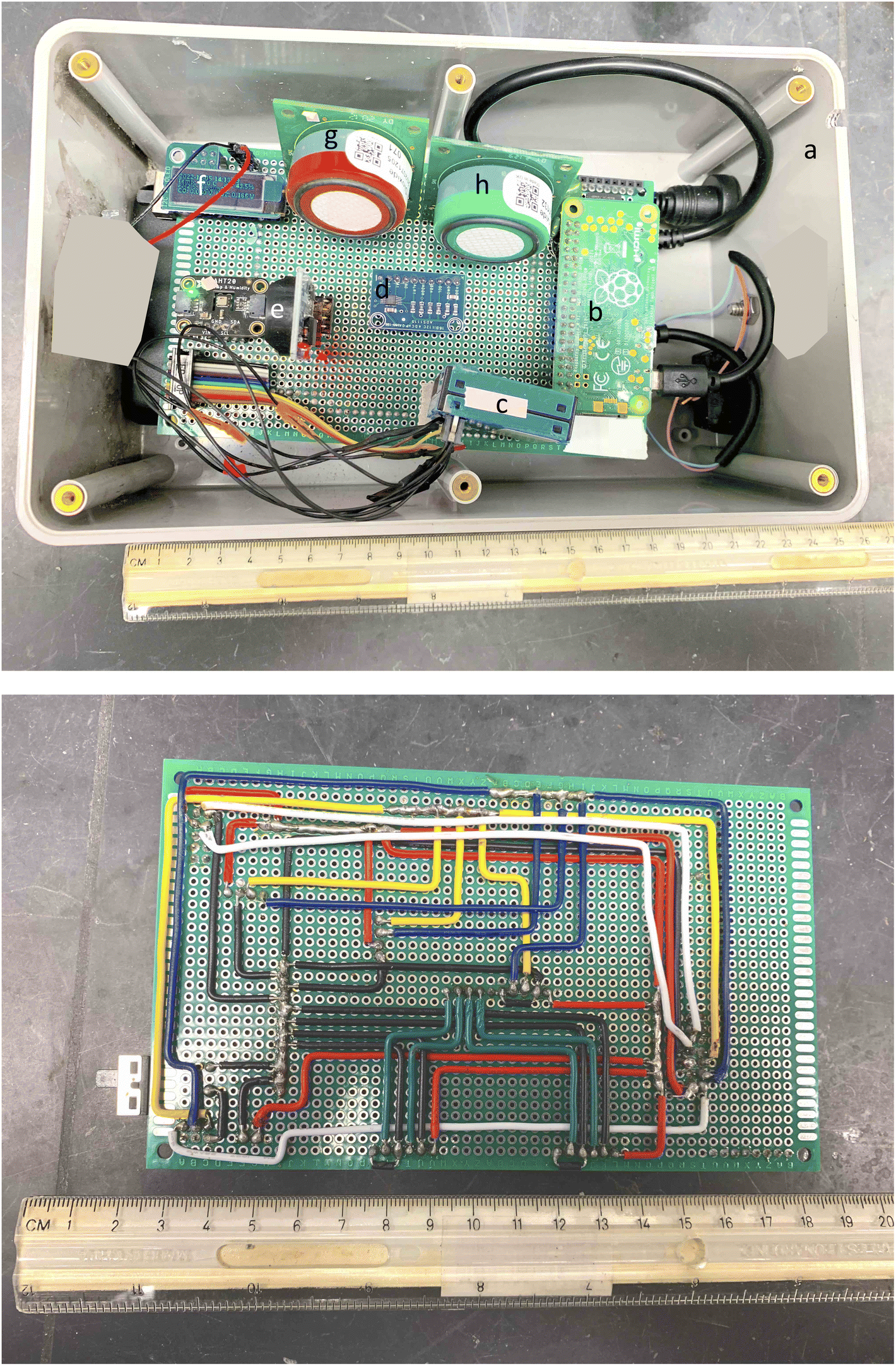Fig. 2 (A) Photograph of sensor circuit board with components (a) plastic box, (b) Raspberry Pi computer, (c) PM_2.5 sensor, (d) A/D converter, (e) temperature and humidity recorder, (f) LED, (g) NO₂ sensor, (h) CO sensor. (B) Back of circuit board with wiring.

Fig. 2B shows the hand wiring connecting power and data lines to battery and the Raspberry Pi microcontroller. The air quality sensors require 5 V, a small LED screen draws 3 V. Data is logged every second, averaged to a single value every minute. Battery life is advertised at 26 000 mA h; but our system, which draws ∼0.5 A, only lasted for ∼30–40 hours.

Sensor box and pumps

The box containing the sensors and battery is plastic, 8 × 12 × 20 cm with a lid sealed by gasket and 6 bolts. We drilled inlet holes for the two tubes used in this design and sealed the through-holes with silicone sealant. An on/off switch was also wired into the board and this switch was also sealed on the side of the box. A small venting hole was also drilled into the box on the end opposite to the inlet tube holes. The volume of this sensor box is about 1.5 L.

Two air pumps (BAENRCY air pump 5–6 vDC) were wired to the power source and controlled by the Raspberry Pi to switch on/off alternatively on a 15 minute cycle. Each air pump is connected to the box housing on the pump outlet side and tubing on the inlet side. One pump has tubing that runs to the tree canopy, the second pump has tubing that runs to a location outside the tree canopy but immediately adjacent. Each pump moves air at ∼1.5 L air per minute.

Calibration

Calibration of sensors was conducted by co-location with higher quality instruments maintained by the South Coast Air Quality Management District (SCAQMD) for 8 days. The calibration was carried out using fitting equations that relate the sensor output (V_WE and V_AE for CO and NO₂, [PM_2.5]_raw for PM_2.5) to the ambient atmospheric concentration (CO and NO₂ in ppm, PM_2.5 in μg m⁻³) taking into account specific meteorological conditions such as temperature and humidity (eqn (1)–(3)). As described below, WE denotes working electrode and AE auxiliary electrode. Meteorological variables and the type of fitting function added to the final model was determined step-by-step. At each step, one variable that appeared to be related to the difference between the corrected sensor signal and the reference was identified, and the relationship was established. This iteration was continued until the best fit of the SCAQMD data was achieved. No significant cross-sensitivity to other pollutants were observed. For CO and NO₂ that involved the use of 8 fitting parameters (k₁–k₈). For PM it only took 3 fitting parameters (k₆–k₈)

CO = k₁ × V_WE − k₂ × V_AE − exp(k₃ × (T − k₄)) − (k₅ × H − exp(k₆ × (H − k₇))) − k₈ (1)

NO₂ = k₁ × V_WE − k₂ × V_AE − exp(k₃ × (T − k₄)) − (k₅ × H − exp(k₆ × (H − k₇))) − k₈ (2)

PM_2.5 = [PM_2.5]_raw − exp(k₆ × (H − k₇)) − k₈ (3)

Values for these fitting parameters are in Table 2. In these Alphasense sensors, CO and NO₂ diffuse through a membrane into an electrolyte where it comes into contact with a working electrode (WE). Additionally, the sensor features an auxiliary electrode (AE) that shares the same catalyst structure as the working electrode but is isolated from the ambient environment. Ideally, subtracting auxiliary voltage (V_AE) from the working voltage (V_WE) would yield a signal that is directly proportional to ambient gas concentration. However, in reality, we have discovered that V_AE in most sensors are unable to accurately follow the variations in V_WE. Temperature (T) and humidity interference (H) should be corrected allowing for a nonlinear effect.⁹ To correct the humidity interference, absolute humidity is calculated from observed temperature (T) and relative humidity (RH) by combining the August–Roche–Magnus approximation of the Clausius–Clapeyron relation (eqn (4)) and the ideal gas law for water vapor (eqn (5)):

P_H2O = H × R_H2O × T (5)

Here, P_H2O, H, and R_H2O are the partial pressure of the water vapor in the atmosphere (in hPa), absolute humidity (in g m⁻³), and specific gas constant of the water vapor (461.52 J kg⁻¹ K⁻¹ = 4.6152 × 10⁻³ hPa m³ g⁻¹ K⁻¹), respectively. We use a nonlinear least square fitting to determine coefficients, k_1–8, by minimizing the difference between the calibrated sensor signal and the SCAQMD reference values (Table 2 and Fig. 3). For CO, NO₂, and PM_2.5, the concentration measured agrees reasonably well with the reference instrument with MBE less than 0.001 ppm, 0.001 ppm, and 0.1 μg m⁻³ and RMSE of 0.1 ppm, 0.006 ppm, and 3.2 μg m⁻³, respectively. R-Squared value is 0.83 for CO, 0.84 for NO₂, and 0.59 for PM_2.5. Table 3 shows the increase in R-squared values when temperature and humidity corrections are considered. Negative R-squared value indicates that excluded correction is necessary to provide feasible calibrated data.

Table 2 Coefficients derived from nonlinear least squares fitting of eqn (1) to SCAQMD reference data. The units of RMSE are ppm for CO and NO₂ and μg m⁻³ for PM_2.5. Mean Bias Error (MBE) included

Sensor	k 1	k 2	k 3	k 4	k 5	k 6	k 7	k 8	MBE	RMSE
CO	2.1	1.6	4.3 × 10^−1	16.3	−3.4 × 10^−3	−3.5 × 10^−1	8.3	8.1 × 10^−2	<0.001	0.1
NO2	2.8	0.0	2.2 × 10^−1	30.3	−2.2 × 10^−3	−4.1 × 10^−1	2.6	7.2 × 10^−1	<0.001	0.006
PM2.5						1.0	10.4	−6.6	<0.1	3.2

---

Fig. 3 Time series and direct comparison of the tree sensor data (blue line) and the SCAQMD reference data (black line). The tree sensor data shown here is optimized to a best fit to the SCAQMD data. The red lines in the plots on the right indicate the 1 : 1 line between these two data. R-Squared values are 0.83, 0.84, and 0.59 for CO, NO₂ and PM_2.5, respectively.

Table 3 R-Squared values for different calibration schemes

Sensor	Without T & H correction	Without T correction	Without H correction	With T & H correction
CO	0.67	0.79	0.72	0.83
NO2	<0	0.41	<0	0.84
PM2.5			<0	0.59

---

Defining uncertainties

While calibrations are essential to understand absolute values of air quality constituents, the question we ask about tree canopy impact can be answered if the sensor results accurately address the difference between constituents in and out of tree canopies. We verified this relative accuracy by co-locating both inlet tubes in ambient air. The results of this colocation (Fig. 4) show some variability (shown as the difference between values measured during draw through one tube vs. the other) and we use this variability to define the uncertainty associated with this methodology. When both tubes are co-located, the difference should be zero. Variation about zero shows the effects of tube contamination/artifact and/or limitations in the performance of the low-cost sensors. However, as discussed below, a major reason for offset between readings from tube 2 to tube 1 during co-location are changes that occur in ambient air on a timescale and magnitude such that our sampling program does not capture these fluctuations. Based on co-location experiments, we assign uncertainties of ±0.5 μg m⁻³, ±0.02 ppm, and ±0.0015 ppm for PM_2.5, CO and NO₂ respectively. During this co-location, ambient air PM_2.5 ranged from 0 to 20 μg m⁻³, ambient CO ranged from 0 to 0.70 ppm and NO₂ ranged 0.005–0.04 ppm.

Fig. 4 Ten-day co-location data showing the difference between values measured in tube 2 minus tube 1. The expected difference for co-location would equal 0. Red shaded area denotes the ± uncertainty assigned to each measurement. >90% of the data are included within the shaded area. (a) PM_2.5 ± 0.5 μg m⁻³. (b) CO ± 0.02 ppm (c) NO₂ ± 0.0015 ppm.

We tested various types of tubing to avoid artifacts associated with gas loss or gain during transport through the tubing and PM loss or gain, the latter being a more serious problem. Tubing with a larger inner diameter is preferred to minimize surface area of tubing inner wall to volume. Various tubes we tested showed demonstrative uptake of PM_2.5, presumably adhering to tubing walls. We found that the best tubing for this application is Synflex, which has an ID of 6.3 mm and 9.5 mm OD and has a nylon-lined inner wall and aluminum reinforced plastic outer wall. We used tubing of equal lengths for tubes #1 and 2, both approximately 10 m.

Programming and data collection

It is essential to consider air flow rate and mixing when moving air into a box containing sensors. At the pump rate described, the entire volume of air inside the sensor box is displaced by pumping for less than 70 seconds. The pump is programmed to move air through one tube for 15 minutes and then the second tube for 15 minutes, alternating for the duration of the experiment (Fig. 5). For the first 5 minutes after switching between tubes, we are recording data but do not use this data because we want the box completely flushed and the sensors to reach a stable reading, which we assume occurs after >4–5 volumes are passed through the box. Readings taken during the subsequent 10 minute period are averaged. The sequence of data generated by our program is as follows: turn on pump, flush 5 minutes, take 10 minute average reading, switch pumps, flush 5 minutes, take 10 minute average, and repeat. We take the difference between the reading of one pump to the average of the prior and post readings of the other pump. This alternation continues; hence it takes 45 minutes to collect data that represents one point for comparison but because of overlap, data points represent a 30 minute sliding window; i.e. every data point represents the difference between one 10 minute average compared to two 10 minute averages.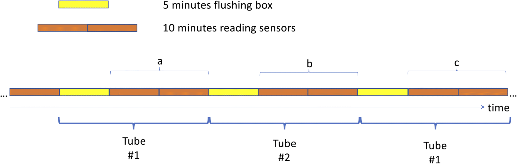

Fig. 5 Schematic of sampling from sensor box. Pumps switch every 15 minutes between tubes 1 and 2. The first 5 minutes after switching is spent flushing out the box, the next 10 minutes data is recorded and averaged. Data is assessed by plotting the average of interval (b) minus the average of intervals (a) and (c). This ‘box car’ sampling continues for the duration of the experiment.

The concentration of constituents in air can be changing while this pump box is switching between tree and no-tree conditions, and this natural variability can generate offsets between these two readings that does not reflect changes occurring due to the location of the sampling tube. By sampling prior and post time intervals, we are assuming that any change in constituent concentration is roughly linear through this 45 minute period. Ambient concentrations sometimes vary or change slope (increasing to decreasing or vice versa) over this time thus we add a correction to take into account these fluctuations. If the slope between reading (a) and (b) is >2 times the slope between (b) and (c) readings (Fig. 5), we cull this data from our comparison. In this way, we are avoiding biases in our data created by rapid changes in ambient air quality and not related to the difference between tree canopy air and ambient.

There is a trade-off between the duration of pumping and the degree to which the sensor box is flushed of previous air and the potential artifact discussed above; longer intervals between switching pumps allows for greater flushing of the box. But longer intervals between switching pumps provides lower resolution in detecting differences between air within and outside the tree canopy. One solution is to use pumps that draw air at a faster rate. This would both minimize time air spent in the tubing but also flush out the sensor box more rapidly. Yet faster pumps draw more power. We find that pump interval durations of 7–15 minutes yield identical results so that we could have gone with shorter pump intervals and generated higher time-resolved data, but the outcome would be the same. If pump times are shorter than 7 minutes, the sensors do not have enough time to come to a stable reading after the box is completely flushed out.

Emplacement of sensors in trees

Different trees have different sizes and shapes to their canopy so systematizing where the inlet tube is placed is an important consideration. We aimed to place the inlet tube close to the tree trunk in a location 3–6 m above ground level. We placed the tube sampling ambient air outside of the tree canopy at 3 m above ground level. The sensor box is located on a supporting pole that holds tube #2 (sampling ambient air) above ground level (Fig. 1). Approximately 10–20 m of tubing will be needed for both sample tubes. Experiments ran for approximately 30–40 hours (battery life) to capture diurnal changes. We have recently added a solar panel to our design and place the panel on a Unistrut in a location outside the tree canopy and hang the sensor box and tube #2 underneath the solar panel. With this panel, experiment lifetime can be infinite.

Air flow around and in a tree canopy will vary and the tree's physiology also varies from day-to-night and due to other environmental stressors. Thus, a single, short-term measurement is unlikely to capture the average condition of tree canopy air quality vs. surrounding air quality. For testing this system, we aimed for comparisons for >24 hours to include the overnight period when Los Angeles wind speeds decrease. Comparing tree canopy to ambient air for extended day/night cycles during different seasons and in different trees (of the same species) is recommended for the most robust test of how a particular tree species influences air quality. Such experiments are in progress.

Data examples

Los Angeles almost always has a strong diurnal fluctuation in air quality parameters due to the expansion of the planetary boundary layer during the daytime and compression overnight.⁶ Overnight AQ constituent levels are higher than during the day due to ground-level source of pollutants and trapping by the boundary layer. The average windspeed is also lower during the night (Fig. 6) and thus the residence time of air within a tree canopy will likely be longer. Assessing air residence time was beyond the scope of this study and not easily parameterized, but any comparison of tree canopy air to ambient air must take into account wind-speed conditions and canopy density.

Fig. 6 (A) Difference between PM_2.5 in ambient air (tube 2) and tree canopy air (tube 1) vs. time. Tubes are co-located following the time indicated by the vertical red line. Dashed line is a 4-point running average. (B) Wind speed during the PM_2.5 experiment (C) same as (A) but for CO. (D) Wind speed during the CO experiment. (E) The difference between NO₂ in ambient and tree canopy air. Dashed line is a 4-point running average.

PM_2.5

A comparison of PM_2.5 from June 6, 2022, differs by time of day (Fig. 6A). During daylight hours, PM_2.5 in the tree canopy was not significantly different from air outside the tree canopy. Beginning around 1800 local time, when the difference between tube 2 and tube 1 (no tree − tree) was negative and outside the uncertainty band. This means particulate matter in the tree canopy air was higher than in the ambient air. PM_2.5 in the tree canopy was elevated by approximately 0.5–1.0 μg m⁻³ that persisted until nearly 0600. A change in windspeed was not the reason the PM_2.5 values in the tree canopy converged with values of ambient air as wind speeds were still low during early daylight hours (Fig. 6B). Based on this single experiment, we'd predict that this particular tree showed diurnal fluctuation in PM production.

Some trees emit volatile organic compounds which can act as precursors for particle formation.¹⁰ It is possible that during the time we conducted these measurements, this tree was emitting precursors enabling the formation of particulate matter. The production and release of pollen is also a possible source of tree PM. That we documented a temporal pattern in PM emission needs to be verified with many more measurements, but also signals physiological and environmental controls on PM production which should be considered when interpreting these results.

CO

Carbon monoxide can be taken up by the stomata of a tree leaf¹¹ and if this happens at a high enough rate, the tree canopy air could show lower CO than the surrounding air. The data from a tree sampled in May 2022 shows this pattern (Fig. 6C). For the duration of this experiment, from 1600 to 0900 the next day, this tree canopy CO values are 0.06 ppm lower than the ambient air. This offset occurs both when CO levels are low (daytime) and high (nighttime). Once the tubes were co-located, the difference converged to 0.

NO₂

One tree we tested showed a diurnal pattern in NO₂ differences between tree canopy and ambient air (Fig. 6E). Readings exceeded the uncertainty range indicating lower values of NO₂ in the tree canopy in the nighttime and higher values in the tree canopy during the daytime as compared to ambient air values. The elevated values we observed may be consistent with results published by Harris and Manning, 2010 (ref. 12) who also found elevated NO₂ values in tree canopies, although it isn't clear what time of day their measurements were made. Because NO₂ is involved in such a complicated set of biogeochemical reactions, monitoring for several day/night cycles would be recommended.

Discussion

There are a number of ways this system could be improved, and air quality impact of trees tested more rigorously. We recommend conducting experiments for a longer duration and for the same species of tree but at different locations. As part of this study, we tested the same tree three times. In April, May and June 2022 a Deodar Cedar tree on USC's campus consistently emitted PM_2.5 during the evening hours. On only one of those test dates did the tree consume CO, the other dates it did not. This example illustrates the importance of making multiple measurements of the same tree, same location, and same tree in other locations in order to take into account the most representative measure of tree performance.

Aside from diurnal changes in tree physiology, there are also seasonal variations that are important to consider. While Los Angeles climate does not change dramatically, there is a still a seasonal temperature and moisture variation. The best measurements of tree canopy impact on air quality will include seasonal measurements and including trees of different ages.

Location of the inlet tube placed in the tree canopy and outside the tree canopy might make a difference to the data outcome. Some trees don't have foliage until quite a great distance off the ground. Testing such a tree would require getting the inlet tube high enough to sample air from within the canopy. Many urban trees, those in Los Angeles, are not so tall and a 3–5 m inlet location is usually going to be within the tree canopy, surrounded by foliage. Systematizing the location of the inlet, as mentioned, can be achieved by attaching the inlet tube to an extendable rod and fastening this rod to the tree trunk.

The location of the inlet tube sampling ambient air should ideally be upwind from the location of the tree, but only just outside the tree canopy. Testing a tree in a densely vegetated area with many surrounding trees may not be ideal. Testing a solidary tree is easily achieved in most urban settings.

The co-location of both inlet tubes is essential to establish that the system is not creating any artifactual data. This could come about via electronic interferences, PM generation or consumption by the tubing and pump materials, or other sources. Taking a time-integrated sample is also important so as to minimize the impact of what might be a short-lived biological event occurring near the inlet tube, e.g. squirrel chasing squirrel or simply patchiness in AQ. Clearly the physiology of trees changes between day and night, so making measurements across both time periods is essential. Tree physiology also changes due to tree stressors, such as heat and/or water supply. Measuring tree canopy air quality as a function of tree physiological state could be a future application for such a system as we are well aware that climate change impacts will affect tree physiology.

Summary/future directions

The low-cost sensor system described here can help quantify tree performance in regard to mitigating or exacerbating air quality. However, to consider trees with respect to overall air quality, one must consider the volume of air encountering trees compared to the overall volume of air and the passage of air through the tree canopy. Ideally, AQ constituent fluxes per tree would be the quantity we'd like to apply to atmospheric chemistry models.

Yet there is value in the static measurements we make as illustrated by this example. Assume an air volume of 1 km × 1 km × 300 m. In this example, 300 m represents an arbitrary planetary boundary layer height. Urban tree density is often counted as trees per length of roadway, 1–10 trees per 100 m is a typical range of values.¹³ However, a large fraction of urban trees are on private property thus we use areal values for Los Angeles from Gillespie et al., 2012 (ref. 14) for this calculation, 10 000 trees per km² (which is larger than counts made in and around downtown Los Angeles by the USC Urban Tree Initiative (https://publicexchange.usc.edu/urban-trees-initiative/) that show tree densities between 1600 and 4000 trees per km²). If we further assume an average tree canopy height of 10 m and it occupies a volume defined by a cylinder 10 m diameter, then the volume of air within a single tree canopy is 785 m³. Thus, the total volume of air contained within tree canopies in this hypothetical example is 7 850 000 m³. This tree canopy volume exists within a total volume of air = 300 000 000 m³. Tree canopy air represents 2.6% of the total ‘hypothetical’ volume. If the ambient air had a PM_2.5 concentration of 15 μg m⁻³ and the trees increased the PM_2.5 by 1 μg m⁻³, their impact on air concentration would be to increase ambient values to 15.03 μg m⁻³.

Of course, this is a ‘static’ calculation, which assumes that there is only air in contact with tree canopy and air that is not in contact with tree canopy within our hypothetical volume. In reality, air is always moving and mixing. A better way to achieve a quantification of how a tree will impact air quality will be to know the residence time that air is in contact with a tree canopy. This will depend on the density of the canopy and the velocity of the wind. Such a determination is necessary to scale this static measurement to a more realistic flux value.

This calculation showing the potential impact of trees on air quality is consistent with recent studies that do not show significant differences in air PM concentration between urban tree areas and open areas.^5,15 Whether this is due to the density of trees, the volume of well mixed air that is not in contact with trees, or tree emission/consumption rates (kinetics) are all very important considerations. The sensor system we describe is intended for use to help quantify tree canopy impact on air constituents and thereby enhance our understanding and ability to quantify the potential benefits of urban trees.

Conflicts of interest

There are no conflicts to declare.

Acknowledgements

We appreciate the cooperation and assistance of SCAQMD personnel Rene Bermudez, Albert Dietrich and Juan Garcia for giving us access to their downtown Los Angeles monitoring site. Funding for this work was provided by USC Dornsife Public Exchange. We acknowledge the support of Kate Weber and Marianna Babboni.

References

1. D. J. Nowak, D. E. Crane and J. C. Stevens, Air pollution removal by urban trees and shrubs in the United States, Urban For. Urban Green., 2006, 4, 115–123.
2. E. G. McPherson, J. R. Simpson, P. F. Peper, S. E. Maco and Q. Xiao, Municipal forest benefits and costs in five U.S. cities, J. For., 2005, 104, 411–416.
3. G. Churkina, F. Kuik, B. Bonn, A. Lauer, R. Grote, K. Tomiak and T. M. Butler, Effect of VOC Emissions from Vegetation on Air Quality in Berlin during a Heatwave, Environ. Sci. Technol., 2017, 51, 6120–6130.
4. R. Grote, R. Samson, R. Alonso, J. H. Amorim, P. Carinanos, G. Churkina, S. Fares, D. Le Thiec, U. Niinemets, T. Norgaard Mikkelsen, E. Paoletti, A. Tiwary and C. Calfapietra, Functional traits of urban trees: air pollution mitigation potential, Front. Ecol. Environ., 2016, 14(10), 543–550.
5. D. E. Pataki, M. Alberti, M. L. Cadenasso, A. J. Felson, M. J. McDonnell, S. Pinceti, R. V. Pouyat, H. Setälä and T. H. Whitlow, The benefits and limits of urban tree planting for environmental and human health, Front. Ecol. Evol., 2011, 9, 603757,  DOI:10.3389/fevo.2021.603757.
6. D. A. Rahn and C. J. Mitchell, Diurnal climatology of the boundary layer in southern California using AMDAR temperature and wind profiles, J. Appl. Meteorol. Climatol., 2016, 55, 1123–1137.
7. J. Kim, A. A. Shusterman, K. J. Lieschke, C. Newman and R. C. Cohen, The Berkeley atmospheric CO2 observation network: Field calibration and evaluation of low-cost air quality sensors, Atmos. Meas. Tech., 2018, 11, 1937–1946.
8. A. A. Shusterman, V. E. Teige, A. J. Turner, C. Newman, J. Kim and R. C. Cohen, The Berkeley atmospheric CO2 observation network: Initial evaluation, Atmos. Chem. Phys., 2016, 16, 13449–13463.
9. M. T. Mead, O. A. M. Popoola, G. B. Stewart, P. Landshoff, M. Calleja, M. Hayes, J. J. Baldovi, M. W. McLeod, T. F. Hodgson, J. Dicks, A. Lewis, J. Cohen, R. Baron, J. R. Saffell and R. L. Jones, The use of electrochemical sensors for monitoring urban air quality in low-cost, high-density networks, Atmos. Environ., 2013, 70, 186–203.
10. L. Liu, B. C. Seyler, H. Liu, L. Zhou, D. Chen, S. Liu, C. Yan, F. Yang, D. Song, Q. Tan, F. Jia, C. Feng, Q. Wang and Y. Li, Biogenic volatile organic compound emission patterns and secondary pollutant formation potentials of dominant greening trees in Chengdu, southwest China, J. Environ. Sci., 2022, 114, 179–193.
11. R. G. S. Bidwell and D. E. Fraser, Carbon monoxide uptake and metabolism by leaves, Can. J. Bot., 1972, 50, 1435–1439.
12. T. B. Harris and W. J. Manning, Nitrogen dioxide and ozone levels in urban tree canopies, Environ. Pollut., 2010, 158, 2384–2386.
13. N. Smart, T. S. Eisenman and A. Karvonen, Street tree density and distribution: An international analysis of five capital cities, Front. Ecol. Evol., 2020, 8, 562646,  DOI:10.3389/fevo.2020.562646.
14. T. W. Gillespie, S. Pincetl, S. Brossard, J. Smith, S. Saatchi, D. Pataki and J.-D. Saphores, A time series of urban forestry in Los Angeles, Urban Ecosyst., 2012, 15, 233–246,  DOI:10.1007/s11252-011-0183-6.
15. H. Setälä, V. Viippola, A.-L. Rantalainen, A. Pennanen and V. Yli-Pelkonen, Does urban vegetation mitigate air pollution in northern conditions?, Environ. Pollut., 2013, 183, 104–112.

---