In situ drift correction for a low-cost NO2 sensor network†
Received
31st October 2022
, Accepted 22nd March 2023
First published on 29th March 2023
Abstract
Twelve low-cost NO2 sensors (LCSs) underwent multiple bi-weekly collocations with a NO2 reference monitor to develop a robust calibration model unique to several periods throughout a summer deployment (April 2021, to October 2021). It was found that a single calibration based on an initial two-week collocation would not hold up in the variable environmental conditions that Phoenix, Arizona experiences in the summer. Temperature, relative humidity, and ozone prove to be critical parameters that would need to be corrected for in the calibration model. Therefore, we developed a period-specific calibration that is re-trained every six weeks to better account for the conditions during that period. This calibration improved sensor performance compared to the sensor manufacturer calibration, yielding an average root-mean-square error (RMSE) of 3.8 ppb and an R2 of 0.82 compared to 19.5 ppb and 0.42 when evaluated against reference NO2 measurements. This improved calibration allowed for more accurate NO2 measurements utilizing LCSs in a sensor network that would not be possible from the out-of-the-box calibration.
Environmental significance
Recent technological advances and heightened public awareness regarding air quality have increased the use of low-cost air quality sensors (LCS), however the precision and accuracy of these devices do not measure up to conventional instrumentation. In this work we developed a calibration method for a network of NO2 LCSs using relative humidity, temperature, and ozone parameters. We found that training the calibration model using data similar to deployment conditions was crucial in improving LCS performance. This required a bi-weekly sensor rotation between deployment and collocation sites, which may not be feasible for larger networks. However, this study does demonstrate the downsides of using LCSs out of the box and the importance of using a calibration relevant to deployment conditions.
|
1 Introduction
According to the World Health Organization (WHO), in 2019, 99% of the world's population was living in areas where air quality guideline levels were not being met, while in 2016, 4.2 million premature deaths were attributed to poor outdoor air quality.1 Although the majority of these deaths were due to PM2.5 (fine particulate matter), nitrogen dioxide gas (NO2) is also a concern, as it's the main source of nitrate aerosols (an important fraction of PM2.5) and a precursor to ozone.2 NO2 is a by-product of fossil fuel combustion from cars, trucks, power plants, and industrial sources.3 The WHO's 2021 24 h NO2 guideline value is 25 μg m−3 (13.3 ppbV), while the U.S Environmental Protection Agency's (EPA) current National Ambient Air Quality Standard (NAAQS) for 1 h NO2 is 100 ppbV.1,4 In order to ensure these guidelines and standards are met, government and community agencies set up monitoring stations at select sites in their region to measure these air pollutants. However, the high financial and logistical costs associated with these monitoring stations limit their spatial resolution and community coverage.
Recent advances in micro-nanotechnology and electronics are driving a new generation of smaller, lower-cost NO2 sensors using metal oxide semi-conductors, and electrochemical cells. While metal oxide semi-conductors have a weak response to NO2 at room temperature and require a recovery time after measurement, electrochemical cells provide a continuous linear output at ambient concentrations.5,6 Many LCS manufacturers such as Clarity Movement Co. (Clarity Movement Co., Berkeley, CA, USA), AQMesh (AQMesh, Stratford upon Avon, UK), and Aeroqual (Aeroqual, Auckland, New Zealand) use electrochemical NO2 sensors in their products. However, these electrochemical cells do have their challenges, as they are often cross-sensitive to gases other than their target, respond to changes in ambient temperature and relative humidity, and degrade over time.6
These low-cost sensors (LCS) can measure some of the same air pollutants that more costly monitors can, but do not provide the same level of accuracy and precision as established measurement systems. To combat this deficiency, LCSs are often collocated with reference monitors to establish calibration models. Despite limitations, low-cost sensors can be an attractive alternative to higher-cost EPA-approved federal reference method (FRM) monitoring because of their cost, size, portability, and ease of use. However, questions remain about how to integrate improved spatial resolution from data collected by LCSs into traditional regulatory monitoring networks, such as the one run by Maricopa County Air Quality Department (MCAQD), so the data can be used to improve the understanding of the causes, extent of impact, and regionality of local air quality issues.
Currently, MCAQD maintains five NO2 monitoring sites that are responsible for covering 10![[thin space (1/6-em)]](https://www.rsc.org/images/entities/char_2009.gif) 322 km2 and serve over 3.3 million people.7 By incorporating nine LCS sites into this network, the average area covered per site decreases from 2000 km2 per site to 700 km2 per site and the average population served from 660 K per site to 235 K per site. For comparison, South Coast Air Quality Management District (SCAQMD), which includes Los Angeles, California, operates 27 NO2 monitoring sites which cover 17428 km2 (645 km2 per site) and 17.5 million people (650 K per site).8 In addition to providing more site-specific data by increasing the network coverage, there are more opportunities to study and better understand pollutant formation routes and behaviors. However, the challenge is ensuring that these LCS networks produce and continue to maintain high quality data. Several studies have already been working on network-specific solutions, such as reference site collocation, transfer standard collocation, remote network calibration, or a proxy model for this data quality issue, most of which recommended semi-regular adjustments to the calibrations to adjust for drift or seasonal bias.9–15 This network management is an additional challenge on top of individual device calibration.
322 km2 and serve over 3.3 million people.7 By incorporating nine LCS sites into this network, the average area covered per site decreases from 2000 km2 per site to 700 km2 per site and the average population served from 660 K per site to 235 K per site. For comparison, South Coast Air Quality Management District (SCAQMD), which includes Los Angeles, California, operates 27 NO2 monitoring sites which cover 17428 km2 (645 km2 per site) and 17.5 million people (650 K per site).8 In addition to providing more site-specific data by increasing the network coverage, there are more opportunities to study and better understand pollutant formation routes and behaviors. However, the challenge is ensuring that these LCS networks produce and continue to maintain high quality data. Several studies have already been working on network-specific solutions, such as reference site collocation, transfer standard collocation, remote network calibration, or a proxy model for this data quality issue, most of which recommended semi-regular adjustments to the calibrations to adjust for drift or seasonal bias.9–15 This network management is an additional challenge on top of individual device calibration.
LCS calibration often involves calibration models that are trained and tested using collocated reference data. These calibration models can include linear regression,9 multivariate linear regression,16 support vector regression,17 generalized additive models,18 random forest models,10 machine learning algorithms,19 or hybrid models.14 For electrochemical-based NO2 LCSs, sensor drift, seasonal bias, ozone cross-interference, and sensor degradation are all issues that should be accounted for in the calibration. Using periodic collocations to re-calibrate the LCSs can address most of these issues as demonstrated in this study. Sun et al.20 attached an additional NO2 removal system to their sensors in order to perform periodic auto-zeroing of their LCSs to correct for drift. Ratingen et al.16 showed that calibrations developed in winter months experience poor performance in summer months with different environmental conditions. Hossain et al.21 have demonstrated the importance of a chemical filter upstream of the electrochemical cell in limiting ozone cross-sensitivity, while Li et al.22 have shown that even with a chemical filter present this scrubber will degrade over time leading to sensor failure. In addition to an ozone scrubber, correcting for ozone interference using site-specific ozone measurements in post-processing calibration has also been performed in several studies.9,11,13,15,16,23
This study seeks to combine network management solutions, such as periodic LCS collocation, with individualized sensor calibration that accounts for temperature, relative humidity, and ozone, to combat sensor drift, seasonal bias, and ozone cross-sensitivity. In this work we were able to deploy 12 LCSs to locations with an O3 EPA-approved federal equivalent method (FEM) instrument to ensure the highest accuracy in our correction for ozone interference. While other sensor network studies have used more sensors in their networks, they did not collocate them all together at a reference site,9,10 by initially co-locating all 12 of our LCSs at a NO2 FRM site we were able to quantify variability among sensors from the same manufacturing run. This allowed us to detect and correct outlier sensors with poor performance compared to the average sensor performance. Additionally, by rotating a few sensors every two weeks to a FRM NO2 site we were able to develop multiple representative training datasets that were used to correct for seasonal bias and changing environmental conditions, which would not be possible with a static network. By maintaining 12 sensors for nine deployment locations, we were able to ensure constant coverage at those sites throughout the deployment period, while providing data with reasonable accuracy (RMSE < 6 ppb) through our robust calibration.
2 Methods
2.1 Instrumentation
Twelve Clarity Node-S model LCSs (Clarity Movement Co., Berkeley, CA, USA), were used in this study to measure hourly NO2 concentrations and were previously evaluated in Miech et al. 2021.23 These LCSs use an Alphasense NO2-A43F electrochemical cell (Alphasense Ltd, Great Notely, UK), which has been shown to have a correctable cross-sensitivity with ozone.22,23 These LCSs were collocated with several NO2 FRM and O3 FEM instruments at 12 Maricopa County Air Quality Department (MCAQD) monitoring sites. The NO2 FRM instrument at the West Phoenix site was a Thermo Scientific 42iQ NO-NO2-NOx Analyzer (ThermoFisher Scientific, Franklin, MA, USA), while the 11 other sites had Teledyne-API T200 (Teledyne API, San Diego, CA, USA), all chemiluminescent based instruments. All 12 sites had a Teledyne-API T400 (Teledyne API, San Diego, CA, USA) to measure ozone via UV absorption. Data from these instruments were obtained from MCAQD at a one-hour resolution.
2.2 Sensor collocation and deployment locations
Table 1 shows the 12 MCAQD monitoring sites that were used in this study, while Fig. S1† shows the spatial layout of the network. These sites were chosen to cover a wide area of Maricopa County, focusing on areas that experience high ozone levels, while avoiding near-roadway sites. All 12 LCSs were collocated at the West Phoenix site for two weeks at the beginning and end of the study (April 12, 2021–April 18, 2021, October 4, 2021–October 19, 2021). During the five-month deployment period the LCSs were rotated between collocation sites, MCAQD sites that measure NO2, and deployment sites, MCAQD sites that only measure O3, every six weeks. This rotation schedule is summarized in Table S1.† This summer period was chosen for the deployment as Maricopa County experiences the majority of its ozone exceedances during this period and the goal of the network was to better understand the NO2 concentration gradient in respect to ozone formation in the region.
Table 1 MCAQD sites used as collocation and deployment locations
| Site name |
Abbreviation |
AQS ID# |
Pollutant measured |
MCAQD site type |
| Blue Point |
BP |
04-013-9702 |
O3 |
Max O3 concentration |
| Buckeye |
B |
04-013-4011 |
O3 & NO2 |
Population exposure and upwind background for O3 |
| Cave Creek |
CC |
04-013-4008 |
O3 |
Max O3 concentration |
| Central Phoenix |
CP |
04-013-3002 |
O3 & NO2 |
Population exposure for O3, highest concentration for NO2 |
| Dysart |
D |
04-013-4010 |
O3 |
Population exposure |
| Mesa |
M |
04-013-1003 |
O3 |
Population exposure |
| North Phoenix |
NP |
04-013-1004 |
O3 |
Max O3 concentration |
| Pinnacle Peak |
PP |
04-013-2005 |
O3 |
Max O3 concentration |
| South Phoenix |
SP |
04-013-4003 |
O3 |
Population exposure |
| South Scottsdale |
SS |
04-013-3003 |
O3 |
Population exposure |
| West Chandler |
WC |
04-013-4004 |
O3 |
Population exposure |
| West Phoenix |
WP |
04-013-0019 |
O3 & NO2 |
Population exposure for NO2 & O3 |
2.3 Calibration models
2.3.1 Original calibration models.
The original calibration models included the sensor manufacturer calibration (SM), the Clarity Baseline calibration, and the Ozone correction model. The SM model calculates NO2 concentrations by using the direct electrochemical cell measurements in an equation provided by the manufacturer (Alphasense Ltd, Great Notely, UK). The Clarity Baseline calibration also uses the electrochemical cell readings combined with the internal temperature and relative humidity measurements in a multivariate regression model to calculate NO2 concentrations. The Ozone correction model uses FEM O3 measurements to correct for the impact of ozone on NO2 concentrations, using the Clarity Baseline Calibration values as a starting point. The SM calibration, Clarity Baseline calibration, and Ozone correction calibration models are detailed in Miech et al.23
2.3.2 Revised calibration model.
Adjustments to the ozone correction model were made incrementally to continue to improve performance measured by minimizing root-mean-square error. With this iteration, there are sensor-specific secondary adjustments for relative humidity, temperature, and ozone, separate calibration factors for daytime (07:00–19:00 labelled NO2Day) and night-time measurements (20:00–06:00 labelled NO2Night), and a correction to force all data above zero. This process is detailed in eqn (1)–(8) and summarized in Fig. S2.† Briefly, all fitting parameters were determined by trial and error to minimize root-mean-squared error between sensor and reference concentration measurements. For eqn (1)–(8), these parameters represent an initial ozone threshold (a), fitting coefficients (c1–7), negative value threshold (b), and final ozone thresholds (d, e). This revised calibration model (Model 1.0) was initially trained by using the full two-week collocation period hourly data at West Phoenix in April 2021.| | | x = ((O3 > a) → (NO2Clarity − (c1 × O3))) ∧ (¬(O3 > a) → NO2Clarity) | (1) |
| | | y = ((x > 0) → (x + (−c2 × RH%))) ∧ (¬(x < 0) → x) | (2) |
| | | z = (y + (c3 × °C)) + c4 | (3) |
| | | w = ((z < 0) → (z + (−c4 × z))) ∧ (¬(z < 0) → z) | (4) |
| |  | (5) |
| | | u = ((0 < v < 1) → (v + (c6 × v))) ∧ (¬(0 < v < 1) → v) | (6) |
| |  | (7) |
| | | NO2Final = ((19 ≤ Hour ≥ 7) → NO2Day) ∧ (¬(19 ≤ Hour ≥ 7) → NO2Night) | (8) |
2.3.3 Revised calibration training.
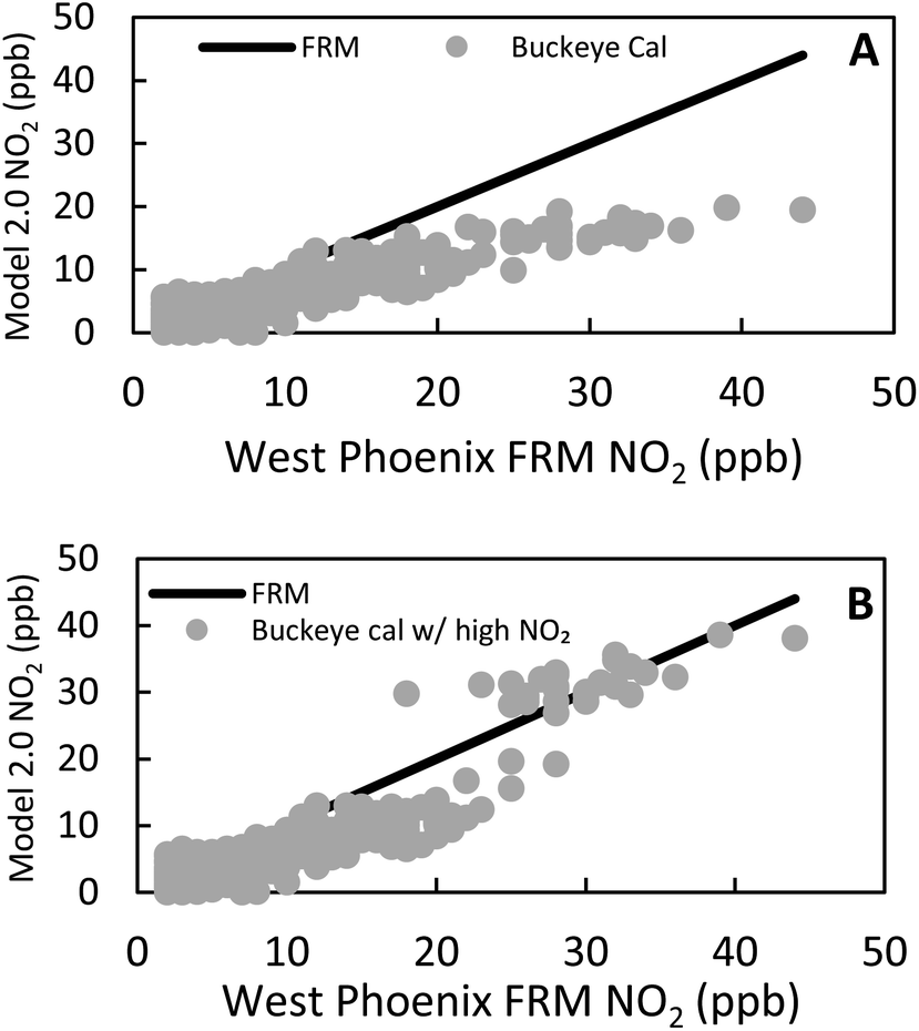
As the study progressed, a need was recognized to periodically re-train the Model 1.0 calibration and the clarity baseline calibration model, as environmental conditions significantly changed throughout the course of deployment. Referred to as Model 2.0, this was accomplished by dividing the LCS deployment into four different periods and re-training the calibration model for each sensor using collocation data from before and after each deployment period. These four weeks of collocation data were then randomized and split 50:50 by day into training and evaluation datasets. Table S2† summarizes these calibration period intervals for the 12 sensors. Using this rotation pattern, the average data loss at each deployment site due to moving the sensors was less than 0.6%. With this method, sensors were now being trained at one of three collocation sites, one of which, Buckeye, exhibited significantly lower (p < 0.05) FRM NO2 values (![[x with combining macron]](https://www.rsc.org/images/entities/i_char_0078_0304.gif) = 5.9 ppb) than the other sites, Central Phoenix ( = 11.1 ppb) & West Phoenix ( = 10.4 ppb). To enable calibration to higher NO2 levels than were routinely observed at Buckeye, we modified the calibration training for sensors 3, 6, 9, and 12 to include several high NO2 datapoints (n = 16) from either the initial or final collocation at West Phoenix in the training datasets that originally only contained Buckeye data. This was incorporated into an additional calibration step, as shown in Fig. S3.†Fig. 1 shows the effect of this inclusion of higher observed NO2 data on a calibration trained at Buckeye and applied to West Phoenix.
= 5.9 ppb) than the other sites, Central Phoenix ( = 11.1 ppb) & West Phoenix ( = 10.4 ppb). To enable calibration to higher NO2 levels than were routinely observed at Buckeye, we modified the calibration training for sensors 3, 6, 9, and 12 to include several high NO2 datapoints (n = 16) from either the initial or final collocation at West Phoenix in the training datasets that originally only contained Buckeye data. This was incorporated into an additional calibration step, as shown in Fig. S3.†Fig. 1 shows the effect of this inclusion of higher observed NO2 data on a calibration trained at Buckeye and applied to West Phoenix.
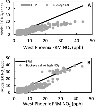 |
| | Fig. 1 Comparison of a (A) Buckeye trained calibration and (B) a Buckeye trained calibration including high NO2 data points applied to Sensor 6 at West Phoenix. | |
2.4 Calibration evaluation methods
To evaluate the performance of the LCSs against FRM NO2 measurements, the root-mean-square error (RMSE), normalized RMSE (NRMSE), Coefficient of Determination (R2), standard deviation, and slope were calculated. Most of these parameters are the recommended performance metrics for O3 air sensors from the EPA's Performance Testing Protocols, Metrics, and Target Values for O3 Air Sensors.24 NRMSE was used to compare accuracy across sites with varying magnitudes of NO2 by dividing the RMSE by average site FRM NO2. Additionally, the Pearson correlation coefficient (r) was used to measure the influence of environmental factors such as relative humidity, temperature, and ozone on the calibration performance.
3 Results and discussion
3.1 Initial calibration performance
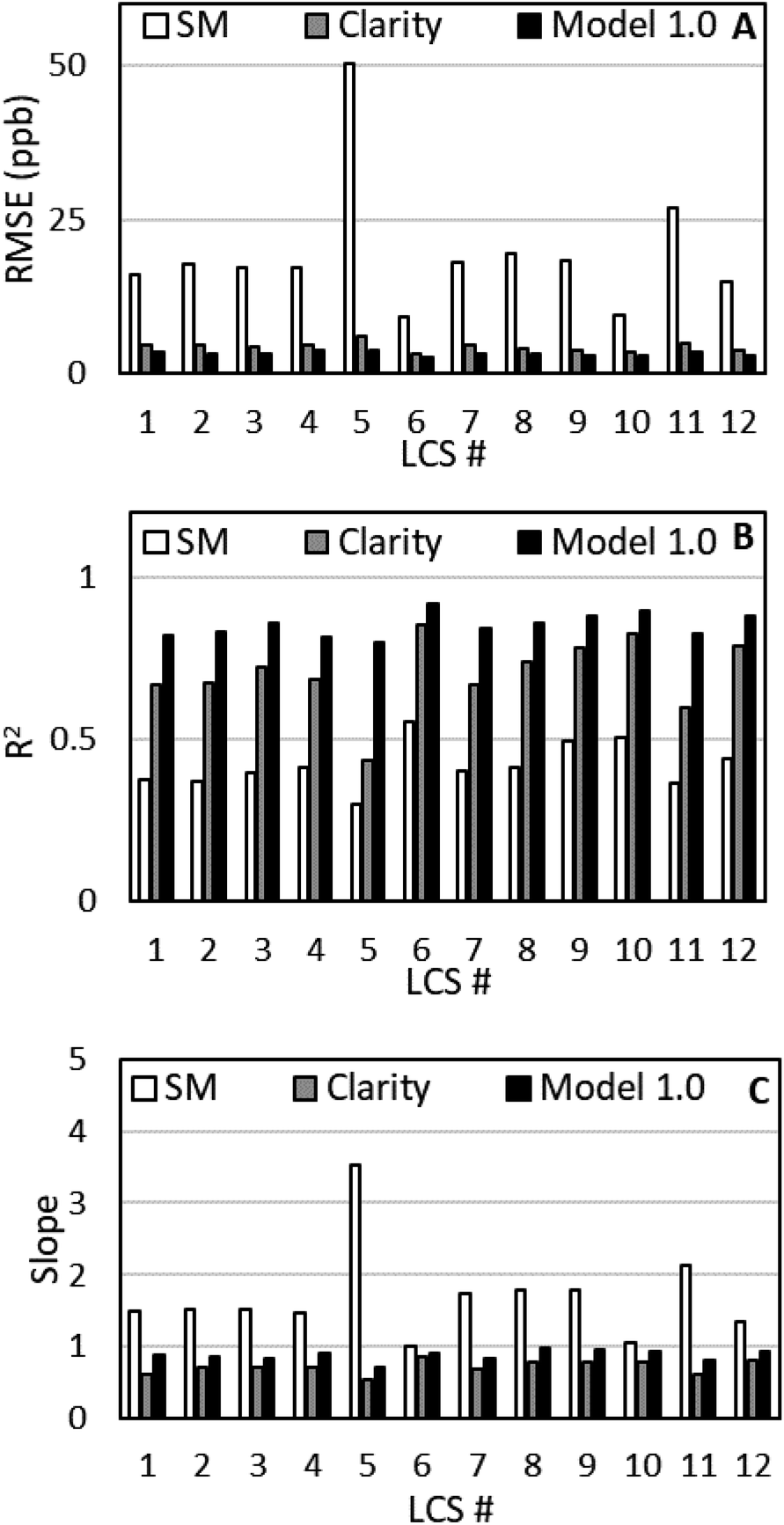
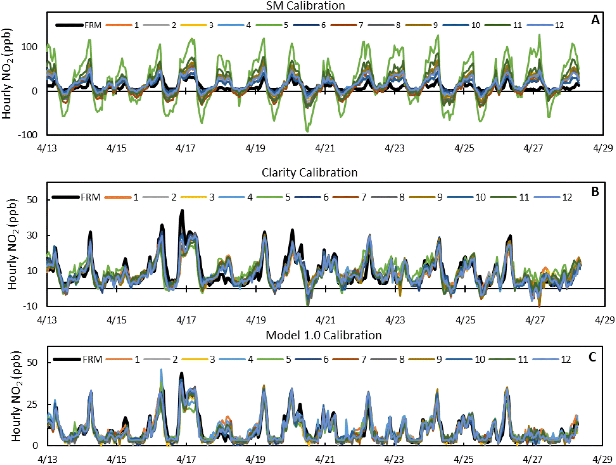
Fig. 2 shows the performance metrics of the SM data, Clarity Baseline model data, and Model 1.0 data trained on April for the initial collocation period, while Fig. 3 show the time series for the calibrations. With the SM calibration model, we see both underprediction at minimum FRM NO2 values and overprediction at maximum FRM NO2 values. This is reflected in RMSE values above 9 ppb, R2 values below 0.6, and variable slopes for all 12 sensors compared to the FRM NO2. Additionally, we see a high average standard deviation, 10.3 ppb, between the sensors; with LCSs #5 and #11 having exceptionally high RMSE and slope values compared to the other 10 sensors, demonstrating inter-sensor variability.
 |
| | Fig. 2 (A) RMSE, (B) R2, and (C) slope values for all 12 sensors based on hourly data over the April 2021 collocation period at West Phoenix using the SM calibration, Clarity Baseline Model, and Model 1.0. | |
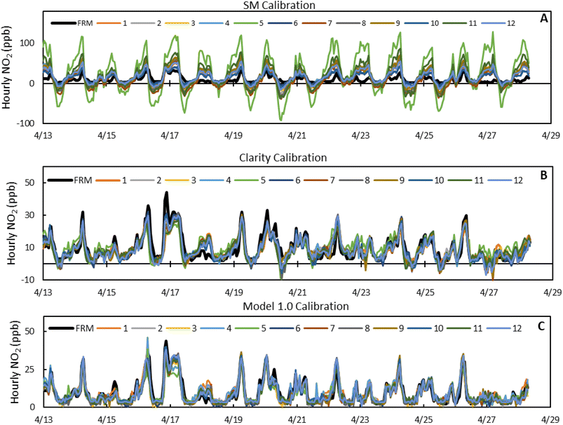 |
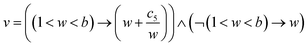
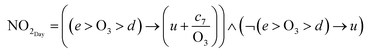
| | Fig. 3 (A) SM calibrated NO2 for all 12 sensors during the April 2021 collocation at West Phoenix. The average standard deviation is 10.3 ppb. (B) Clarity calibrated NO2 for all 12 sensors during the April 2021 collocation at West Phoenix. The average standard deviation is 1.66 ppb. (C) NO2 values using Model 1.0 for all 12 sensors during the April 2021 collocation at West Phoenix. The average standard deviation is 1.65 ppb. | |
By applying the clarity baseline calibration, the model no longer overpredicts at maximum FRM NO2 values, but we still see some underprediction at minimum values and new underprediction at maximum values. Additionally, we see that the average RMSE decreased by 78%, the average R2 increased by 67%, and the average slope improves from 1.679 to 0.719. Furthermore, the standard deviation is reduced to 1.66 ppb and LCSs #5 and #11 have more comparable performance to the other sensors. Using Model 1.0, the underprediction of the clarity baseline model is corrected, as the average RMSE decreased by 25%, the average R2 increased by 21%, and the average slope improves from 0.719 to 0.878 with minimal change in standard deviation.
3.2 Initial calibration performance over time
Throughout the deployment period, the LCSs were periodically collocated at reference monitor sites to verify calibration performance. Their performance is summarized in Fig. 4, where each box is a compilation of three sensors over a two-week collocation period. The average RMSE of the Clarity Baseline model over the whole period was 14 ± 5 ppb, while the average Model 1.0 RMSE was 6.1 ± 0.9 ppb. In addition to the large standard deviation, the Clarity Baseline RMSE had a substantial drift over time, while Model 1.0 was consistent. The R2 values were more similar, with the Clarity Baseline having an average R2 of 0.3 ± 0.2 and 0.5 ± 0.3 for Model 1.0. Both models saw a significant decrease in R2 during the beginning of July and August. Similar trends are seen in the average slopes, where for the clarity baseline it was 0.8 ± 0.3 and for Model 1.0 0.7 ± 0.3, with a decrease in performance at the beginning of July.
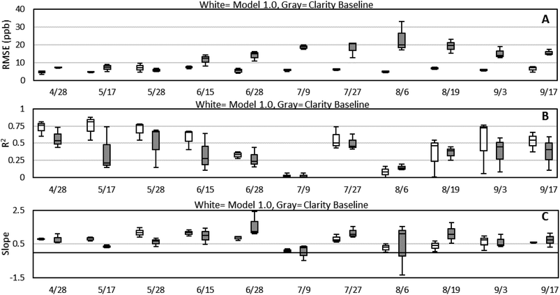 |
| | Fig. 4 Box and whisker plots for the (A) RMSE, (B) R2, and (C) slope values of the Model 1.0 and Clarity baseline calibrated data from each 2 weeks collocation. Each point is a compilation of values from the 3 collocated sensors for that period. The lines within the boxes represent the medians, the interquartile range is the range of the boxes with the top representing the 75th and the bottom the 25th percentile. The whiskers represent the maximum and minimum values in the data. | |
Individual LCS performance and site-specific performance over the deployment period can be found in Fig. S4 and S5.† For the individual LCS performance LCSs #1, #2, #3, #6, #10, and #12 all experienced R2 values below 0.2 and slopes below 0.4 during a period from the beginning of July to the end of August. However, with the Model 1.0 calibration, there were no clear outlier sensors across the whole deployment period, as was seen with LCSs #5 and #11 using the SM calibration. For the site-specific performance, LCSs had lower performances at the Buckeye collocation site compared to West Phoenix and Central Phoenix. To account for magnitude differences in FRM NO2 between the sites, NRMSE was used as a calibration performance parameter instead of RMSE. The average NRMSE at the Buckeye site over the deployment period was 0.9 ± 0.3 compared to 0.7 ± 0.2 and 0.6 ± 0.1 at West Phoenix and Central Phoenix respectively. The average R2 and slope values at Buckeye were 0.3 ± 0.2 and 0.6 ± 0.4 compared to R2 values of 0.6 ± 0.3 and 0.5 ± 0.3 and slopes of 0.8 ± 0.3 and 0.7 ± 0.3 at West Phoenix and Central Phoenix.
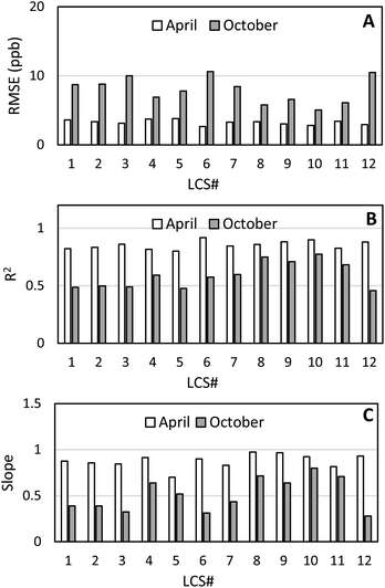
The final October collocation at West Phoenix provided an opportunity to compare the performance of all LCSs to their initial performance during the April collocation. Fig. 5 shows the RMSE, R2, and slope values for Model 1.0 during the April and October collocation. Nearly all 12 LCS RMSE values doubled from April to October, coupled with reductions in R2 and slope. Both the SM calibration and clarity baseline model saw variable results when comparing October to April, shown in Fig. S6 and S7† possibly as these models may not be able to accurately correct for changing environmental conditions. While sensor degradation may play a role in this decreased performance, the environmental conditions that the LCSs experienced may also affected their performance.
 |
| | Fig. 5 (A) RMSE, (B) R2, and (C) slope values for all 12 sensors over the April 2021 and October 2021 collocation periods at West Phoenix using Model 1.0. | |
3.2.1 Impact of environmental factors on calibration performance.
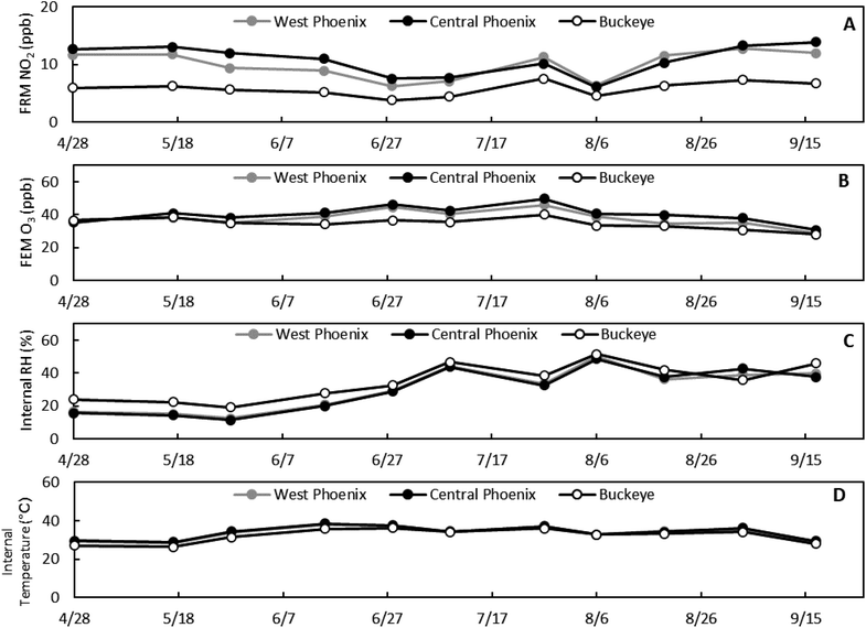
As previously shown, the Model 1.0 calibration performance decreased significantly from the time of calibration in April to the last collocation in October. Additionally, there were periodic decreases in calibration performance throughout the summer, specifically in the beginning of July and August. To better explain these changes in performance we need to examine the environmental conditions at those time points. Doing that also offers the possibility of evaluating a calibration methodology that is based on periodic re-training, i.e. Model 2.0 detailed in Section 3.3. For example, the average hourly FRM NO2, FEM O3, RH, and temperature during the April collocation were 9 ppb, 38 ppb, 20%, and 25 °C, while during the October collocation it was 14 ppb, 25 ppb, 33%, and 24 °C. Fig. 6 shows the average FRM NO2, FEM O3, internal sensor relative humidity, and internal sensor temperature for the three colocation sites for each two-week collocation period. Fig. 6A shows that the NO2 is variable over time with a sharp decrease around 08/06, and as expected the Buckeye site has lower average NO2 values than the more urban Central and West Phoenix sites. Looking at the average FEM O3, it is consistent over time and between the three sites. With internal relative humidity, Fig. 6C, there are peaks around 07/09 and 08/06 at all three sites which may explain the decrease in calibration performance we saw during those same time periods. The average internal temperature does not greatly vary between sites and over time.
 |
| | Fig. 6 (A) Average FRM NO2, (B) FEM O3, (C) internal sensor relative humidity, and (D) internal sensor temperature for each 2 weeks collocation period at the three collocation sites. | |
To confirm whether these environmental factors impacted the performance of the calibrations, we calculated the Pearson correlation coefficients of the average FEM O3, FRM NO2, internal sensor relative humidity, and internal sensor temperature to the RMSE, R2, and slope of Model 1.0 and Model 2.0 calibrations, shown in Fig. 7. For both Model 1.0 and Model 2.0 calibrations the RMSE, R2, and slope correlations to ozone were below |0.3|, therefore the calibration performance is not strongly affected by ozone demonstrating that the ozone correction step in both models is effective. With temperature, there was a decrease in correlation to RMSE, R2, and slope of the Model 2.0 calibration compared to the Model 1.0 calibration, showing that the Model 2.0 calibration may be counteracting any effects temperature has on the calibration performance. This counteracting effect from the Model 2.0 calibration also applied to relative humidity as the correlation between RH and R2 and slope decreased for the Model 2.0 calibration compared to the Model 1.0 calibration. Additionally, we see that relative humidity is one of the factors most strongly correlated to the calibration performance, specifically R2 and slope. This helps explain why we saw decreases in R2 and slope during periods of high RH (07/09 & 08/06) but not an increase in RMSE. Finally, we do see a strong correlation between FRM NO2 and calibration performance for both the Model 1.0 and Model 2.0 calibrations. However, this may be an artifact of the RMSE, R2, and slope calculations which do include FRM NO2 values. Fig. S8† shows the correlations between the environmental variables and NO2 residuals for Model 1.0 and Model 2.0 calibrations where there is little difference between the models.
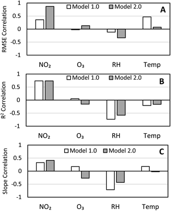 |
| | Fig. 7 (A) RMSE, (B) R2, and (C) slope correlations for the Model 1.0 and Model 2.0 calibrations to FRM NO2, FEM O3, internal sensor relative humidity, and internal sensor temperature. | |
3.3 Period-specific calibration
As noted above, changes in ambient temperature, relative humidity, and ozone result in changes to the calibration parameters of the LCSs. For Phoenix, where seasonal changes in the local weather patterns lead to dramatically different relative humidity levels over the course of the summer, this means that the calibration of LCSs needs to use intercomparison data that is collected contemporaneously with the calibration period. For local conditions, simply using data from a sensor collocation at the beginning of the summer (April) and the end of the summer (October) will not correctly capture the changes in relative humidity that occur with the onset of the southwestern monsoon season. Fig. S3† recaps the entire calibration process (Model 2.0) that we have developed and applied to each sensor, while Table S2† details the interval periods used to calibrate each sensor.
As a comparison to the Model 2.0 calibrated data, we have also analyzed the Model 1.0 calibration using the Model 2.0 evaluation dates for a more equivalent comparison. Fig. 8 shows box and whisker plots of RMSE, R2, and slope for Model 1.0 and Model 2.0 for Periods 1–4. Compared to Model 1.0, Model 2.0 data has a lower RMSE, higher R2, and improved slope during Periods 1–4, in addition to lower variability. While Fig. 8A appears to show an upward drift in RMSE over the periods, the NRMSE values in Fig. 8B demonstrates that this is an artifact of increasing NO2 concentrations throughout the deployment.
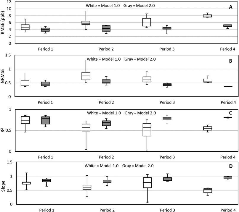 |
| | Fig. 8 Box and whisker plots for the (A) RMSE, (B) NRMSE, (C) R2, and (D) slope values of the Model 1.0 and Model 2.0 calibrated data from each period. Each point is a compilation of values from the 12 sensors for that period. The lines within the boxes represent the medians, the interquartile range is the range of the boxes with the top representing the 75th and the bottom the 25th percentile. The whiskers represent the maximum and minimum values in the data. | |
Fig. S9–12† show the RMSE, NRMSE, R2, and slope values for the twelve individual sensors during the 4 collocation periods. For Period 1, LCSs #7, #8, #9, #10, and #12 with the Model 2.0 calibration, all experienced improvements in RMSE and slope, with an average RMSE reduction of 28% compared to Model 1.0. During Period 2, eight out of the twelve sensors experienced at least a 20% reduction in RMSE, with all experiencing improvements in slope and R2, except for LCS #7. All but one LCS, LCS #1, had at least a 20% decrease in RMSE for Period 3 compared to Model 1.0. Of note, LCSs #3, #6, #9, and #12 were collocated at Buckeye during rotations throughout the summer and at West Phoenix in April and October. For these sensors, we see significant improvement from the Period 3 Model 2.0 calibration when compared to the Model 1.0 calibration. For example, LCS #3 Model 1.0 had a R2 of 0.0094 and a slope of 0.0596, but with the Model 2.0 calibration this improved to 0.6737 and 0.83127 respectively. Finally, for Period 4, all three LCSs that were calibrated during this period experienced lower RMSE values, and higher R2 and slope values closer to unity than Model 1.0. Fig. 9 shows box and whisker plots of RMSE, R2, and slope for Model 1.0 and Model 2.0 by date, using the evaluation dataset. Fig. 9B and C clearly show an improvement in R2 and slope for Model 2.0 during the summer period that Model 1.0 was having trouble with. Fig. S13† directly compares Model 1.0 and Model 2.0 to the FRM data for Period 3, where there is a clear improvement in fit from Model 1.0 to 2.0. Additionally, Model 2.0 is more stable over the entire deployment period with a lower variability compared to Model 1.0. This is consistent with Fig. 7, where we saw the performance characteristics of Model 2.0 were less susceptible to changes in RH and temperature than Model 1.0. Sensor variability is extremely important in this network application since data from multiple sensors will be compiled to produce NO2 measurements from each site across the whole deployment. Fig. S14† demonstrates how seamless the sensor-to-sensor transition is for the Mesa site using Model 2.0 compared to the SM calibrated data.
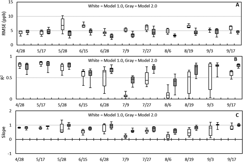 |
| | Fig. 9 Box and whisker plots for the (A) RMSE, (B) R2, and (C) slope values of the Model 1.0 and Model 2.0 calibrated data from two-week periods. Each point is a compilation of values from the 3 sensors collocated during that date range. The lines within the boxes represent the medians, the interquartile range is the range of the boxes with the top representing the 75th and the bottom the 25th percentile. The whiskers represent the maximum and minimum values in the data. | |
4 Conclusion
With an increasing demand for spatially resolved air quality data, low-cost sensor networks have emerged as a possible answer, but are not without their challenges. One of the biggest tasks is to develop a robust calibration that works for the whole network and in a variety of conditions. With our initial Model 1.0 calibration, we demonstrated the importance of developing a calibration capable of correcting for environmental conditions such as temperature, relative humidity, and ozone, for NO2 LCSs specifically. But even with these corrections, we saw a decrease in sensor accuracy throughout the deployment period and at different locations. To counteract this diminished performance, we periodically collocated the LCSs at a reference monitor site and re-trained the calibration model using the periodic collocation data which accounted for the environmental conditions at the time of data collection as opposed to using a single training dataset from the initial deployment. Using this calibration training method, we were able to improve the RMSE, NRMSE, R2, and slope values for the LCSs throughout the deployment period. The final data had an average RMSE of 4.2 ppb, NRMSE of 0.5, R2 of 0.734, and a slope of 0.855, a considerable improvement over the SM calibrated LCS data output. Even with these improvements the LCSs are still at least an order of magnitude lower in terms of resolution and accuracy compared to traditional chemiluminescence instruments, but they make up for this in price, portability, and ease of use. These results highlight the value of training the sensor calibration model on environmental conditions comparable to those expected at and during the deployment period. However, it should be noted that the method used here required bi-weekly trips to rotate the sensors between the collocation and deployment sites, which may not be feasible for larger sensor networks. An ideal solution for larger networks would be a mobile reference instrument that could be rotated between LCS deployment locations for periodic collocation and recalibration.
Author contributions
Conceptualization, J. A. M., M. P. F. and P. H.; methodology, J. A. M., P. M., M. P. F. and P. H.; software, L. S.; formal analysis, J. A. M.; investigation, J. A. M.; data curation, J. A. M. and L. S.; writing—original draft preparation, J. A. M.; writing—review and editing, L. S., J. U., P. M., M. P. F. and P. H.; visualization, J. A. M.; supervision, M. G., M. P. F. and P. H.; project administration, J. U. All authors have read and agreed to the published version of the manuscript.
Conflicts of interest
L. S., P. M. and M. G. are employees of Clarity Movement Co., whose sensors were used and evaluated in this study. At the time of this study J. U. was an employee of Maricopa County Air Quality Department, which provided funding for this work.
Acknowledgements
The authors would like to thank Kanchana Chandrakanthan, Quincy Stewart, and Megan Gaitan for their support with this project's field work and Maricopa County Air Quality Department for funding this work.
References
-
World Health Organization, Ambient (Outdoor) Air Pollution Fact Sheet, World Health Organization, Geneva, Switzerland, 2021 Search PubMed.
- J. N. Galloway, J. D. Aber, J. A. N. W. Erisman, S. P. Seitzinger, R. W. Howarth, E. B. Cowling and B. J. Cosby, The Nitrogen Cascade, Bioscience, 2003, 53(4), 341–356, DOI:10.1641/0006-3568(2003)053[0341:TNC]2.0.CO;2.
-
United States Environmental Protection Agency, Air Quality Guide for Nitrogen Dioxide, 2011 Search PubMed.
-
Environmental Protection Agency, Review of the Primary National Ambient Air Quality Standards for Oxides of Nitrogen, 2018 Search PubMed.
- C. Zhang, Y. Luo, J. Xu and M. Debliquy, Room Temperature Conductive Type Metal Oxide Semiconductor Gas Sensors for NO2 Detection, Sens. Actuator A Phys., 2019, 289, 118–133, DOI:10.1016/j.sna.2019.02.027.
-
M. Raninec, Overcoming the Technical Challenges of Electrochemical Gas Sensinghttps://www.analog.com/en/technical-articles/overcoming-the-technical-challenges-of-electrochemical-gas-sensing.html, accessed Jul 19, 2022 Search PubMed.
-
Maricopa County Air Quality Department, Maricopa County Air Monitoring Network Assessment 2015-2019, 2020 Search PubMed.
-
South Coast Air Quality Management District, Annual Air Quality Monitoring Network Plan, 2022 Search PubMed.
- D. R. Peters, O. A. M. Popoola, R. L. Jones, N. A. Martin, J. Mills, E. R. Fonseca, A. Stidworthy, E. Forsyth, D. Carruthers and M. Dupuy-Todd,
et al., Evaluating Uncertainty in Sensor Networks for Urban Air Pollution Insights, Atmos. Meas. Tech., 2022, 15(2), 321–334, DOI:10.5194/amt-15-321-2022.
-
M. I. G. Daepp, A. Cabral, V. Ranganathan, V. Iyer, S. Counts, P. Johns, A. Roseway, C. Catlett, G. Jancke, D. Gehring, et al., Eclipse: An End-to-End Platform for Low-Cost, Hyperlocal Environmental Sensing in Cities, ACM/IEEE International Conference on Information Processing in Sensor Networks, 2022 Search PubMed.
- J. Hofman, M. Nikolaou, S. P. Shantharam, C. Stroobants, S. Weijs and V. P. La Manna, Distant Calibration of Low-Cost PM and NO2 Sensors; Evidence from Multiple Sensor Testbeds, Atmos. Pollut. Res., 2022, 13(1), 101246, DOI:10.1016/j.apr.2021.101246.
- L. Chatzidiakou, A. Krause, O. A. M. Popoola, A. Di Antonio, M. Kellaway, Y. Han, F. A. Squires, T. Wang, H. Zhang and Q. Wang,
et al., Characterising Low-Cost Sensors in Highly Portable Platforms to Quantify Personal Exposure in Diverse Environments, Atmos. Meas. Tech. Discuss., 2019, 1–19, DOI:10.5194/amt-2019-158.
- M. I. Mead, O. A. M. Popoola, G. B. Stewart, P. Landshoff, M. Calleja, M. Hayes, J. J. Baldovi, M. W. McLeod, T. F. Hodgson and J. Dicks,
et al., The Use of Electrochemical Sensors for Monitoring Urban Air Quality in Low-Cost, High-Density Networks, Atmos. Environ., 2013, 70, 186–203, DOI:10.1016/j.atmosenv.2012.11.060.
- C. Malings, R. Tanzer, A. Hauryliuk, S. P. N. Kumar, N. Zimmerman, L. B. Kara, A. A. Presto and R. Subramanian, Development of a General Calibration Model and Long-Term Performance Evaluation of Low-Cost Sensors for Air Pollutant Gas Monitoring, Atmos. Meas. Tech., 2019, 12(2), 903–920, DOI:10.5194/amt-12-903-2019.
- L. Weissert, E. Miles, G. Miskell, K. Alberti, B. Feenstra, G. S. Henshaw, V. Papapostolou, H. Patel, A. Polidori and J. A. Salmond,
et al., Hierarchical Network Design for Nitrogen Dioxide Measurement in Urban Environments, Atmos. Environ., 2020, 228, 117428, DOI:10.1016/j.atmosenv.2020.117428.
- S. v. Ratingen, J. Vonk, C. Blokhuis, J. Wesseling, E. Tielemans and E. Weijers, Seasonal Influence on the Performance of Low-Cost NO2 Sensor Calibrations, Sensors, 2021, 21(23), 7919, DOI:10.3390/s21237919.
- A. Bigi, M. Mueller, S. K. Grange, G. Ghermandi and C. Hueglin, Performance of NO, NO2 Low Cost Sensors and Three Calibration Approaches within a Real World Application, Atmos. Meas. Tech., 2018, 11(6), 3717–3735, DOI:10.5194/amt-11-3717-2018.
- S. Munir, M. Mayfield, D. Coca, S. A. Jubb and O. Osammor, Analysing the Performance of Low-Cost Air Quality Sensors, Their Drivers, Relative Benefits and Calibration in Cities—a Case Study in Sheffield, Environ. Monit. Assess., 2019, 191(2), 22–94, DOI:10.1007/s10661-019-7231-8.
- K. R. Smith, P. M. Edwards, P. D. Ivatt, J. D. Lee, F. Squires, C. Dai, R. E. Peltier, M. J. Evans, Y. Sun and A. C. Lewis, An Improved Low-Power Measurement of Ambient NO2 and O3 Combining Electrochemical Sensor Clusters and Machine Learning, Atmos. Meas. Tech., 2019, 12(2), 1325–1336, DOI:10.5194/amt-12-1325-2019.
- L. Sun, D. Westerdahl and Z. Ning, Development and Evaluation of a Novel and Cost-Effective Approach for Low-Cost NO2 Sensor Drift Correction, Sensors, 2017, 17(8), 1916, DOI:10.3390/s17081916.
- M. Hossain, J. Saffell and R. Baron, Differentiating NO2 and O3 at Low Cost Air Quality Amperometric Gas Sensors, ACS Sens., 2016, 1(11), 1291–1294, DOI:10.1021/acssensors.6b00603.
- J. Li, A. Hauryliuk, C. Malings, S. R. Eilenberg, R. Subramanian and A. A. Presto, Characterizing the Aging of Alphasense NO2 Sensors in Long-Term Field Deployments, ACS Sens., 2021, 6(8), 2952–2959, DOI:10.1021/acssensors.1c00729.
- J. A. Miech, L. Stanton, M. Gao, P. Micalizzi, J. Uebelherr, P. Herckes and M. P. Fraser, Calibration of Low-Cost NO2 Sensors through Environmental Factor Correction, Toxics, 2021, 9(11), 281, DOI:10.3390/toxics9110281.
-
R. Duvall, A. Clements, G. Hagler, A. Kamal, V. Kilaru, L. Goodman, S. Frederick, K. Johnson Barkjohn, I. Vonwalk, D. Green, T. Dye, Performance Testing Protocols, Metrics, and Target Values for Ozone Air Sensors: Use in Ambient, Outdoor, Fixed Site, Non-regulatory and Informational Monitoring Applications, Washington, D.C, 2021 Search PubMed.
Footnotes |
| † Electronic supplementary information (ESI) available. See DOI: https://doi.org/10.1039/d2ea00145d |
| ‡ Current address: City of Phoenix, Phoenix, Arizona 85003, United States. |
|
| This journal is © The Royal Society of Chemistry 2023 |
Click here to see how this site uses Cookies. View our privacy policy here. 
 Open Access Article
 This Open Access Article is licensed under a Creative Commons Attribution-Non Commercial 3.0 Unported Licence
 a,
Levi
Stanton
a,
Levi
Stanton