Robotically automated 3D printing and testing of thermoplastic material specimens

Abstract

The process of development of new thermoplastic polymers, both with or without property-enhancing additives, requires preparation of test specimens to be used for subsequent characterization of materials' mechanical, fire and other properties. One of the techniques that can be employed to produce such specimens is fused deposition modeling (3D printing) though it is heavily dependent on the processing parameters that need to be adjusted for each considered material. Herein, we present an automated robotized workflow that can take polymer pellets as the input, identify 3D printing parameters to produce quality specimens and perform their mechanical property testing via the Charpy impact test. The workflow involves pellet-based 3D printers working in parallel, a collaborative robot manipulator to handle the printed specimen, a balance and camera vision system to monitor the quality of the specimen, and an analog impact tester instrument, the operation of which has been fully automated with the aid of the robot and do-it-yourself accessories. We investigate two approaches to control the workflow to identify acceptable 3D print parameters. The design of experiment approach, based on Latin hypercube sampling, can identify specimens of sufficient quality within 10 3D prints while Bayesian optimization can reach a comparable quality in fewer experiments and further improve the quality, though this comes at a much higher cost due to the experimental noise (greater or equal than 1%), the required estimation of the hyperparameters and the structure–property relationship.

---

Introduction

Plastics are essential in modern society because of their wide range of applications. Thermoplastics, which represent roughly 75 percent of the market,¹ have been widely employed due to their prominent strength/weight ratio, high processability, corrosion resistance, and low cost. Their properties can be further tuned with additives as well and new functionality can be incorporated into the materials with fillers such as fibers or nanoparticles.

Thermoplastics are currently mainly produced from non-renewable fossil resources as they are largely non-biodegradable. Their disposal leads to the accretion of large amounts of waste, which adversely affects natural ecosystems.² There is an urgent need to address these issues by the development and large-scale adoption of nature-derived, recyclable, and/or biodegradable polymeric materials and their additives. An example of such a biopolymer alternative is polylactide (PLA) which has found more enduring applications in sectors such as automotives and electronics^3,4 while nanoclays and chitosan are examples of sustainable fillers improving mechanical and fire properties, respectively.

A typical scientific approach to the development of novel polymers and their composites entails a large number of tests that are planned based on theory. In circumstances where the theory is not well established, the discovery process usually includes trial-and-error experimentation. Furthermore, for a newly produced functional material to be employed in a specific application, additional optimization stages are required for the material to match the industry's specific needs. Thus, the development of polymer materials and composites becomes costly in terms of time, human resources, and capital. In fact, this same challenge is shared across many other material types and applications, and has led to the introduction of the concept of material acceleration platforms (MAPs), also known as self-driving laboratories.^5,6 MAPs combine the transformational power of artificial intelligence and robotics to allow high-throughput experimentation and analysis of the generated data to minimize the number of experiments needed to optimize the desired properties, reducing the time, economical cost and environmental impact of the experimentation process. While the typical cost for developing a material is calculated to be around 10 to 20 years from initial research to first industry application,⁷ recent reviews estimate that material acceleration platforms can accelerate this pace by 10 to 100 times.⁸ For example, Burger et al.⁹ presented a fully automated laboratory by the use of a mobile robot that was able to find enhanced photocatalysts for hydrogen production from water. The robot was programmed to move in the laboratory and operate the lab equipment, offering a flexible approach to laboratory automation. Bayesian optimization (BO) was used to explore the parameter space and find the most promising candidates for the objective application. BO is a common methodology for global optimization, especially used with expensive-to-evaluate objective functions. BO relies on (i) a continually updated surrogate model to capture the belief about structure–property relationships and (ii) an acquisition function to make sequential decisions of which experimental targets to evaluate next while balancing: (a) exploitation of the available structure–property relationship model based on the experiments conducted thus far to pick up the next experimental target believed to be the optimal one and (b) exploration of regions of the design space where belief about the structure–property relationship is weak, and pick up the experimental targets to strengthen confidence in the model. Such a formulation makes the search both active and efficient, and hence other MAPs have also incorporated the BO framework. MacLeod et al.¹⁰ reported an application, where the composition of thin films is optimized in an automatic way. The samples were created by spin coating and characterized for optical and electronic properties. The software used in this case to orchestrate the experiment and perform the optimization was ChemOS.¹¹ A more recent example of an autonomous laboratory¹² uses Bayesian optimization and an automated workflow to find the optimal ratio in the components for adhesives to maximize the pull-off strength.

Characterization of the properties of thermoplastics typically involves experiments using standardized test specimens at the centimeter scale. These can be produced via various approaches such as injection molding, hot pressing or additive manufacturing (AM). AM's fused deposition modeling (FDM) is widely employed for the fabrication of PLA products and PLA-based multifunctional composites.^13,14 However, the final performance of the printed articles is highly dependent on the parameters and conditions of the AM process, such as environmental conditions, material properties (e.g., density, thermal properties, moisture content, and rheological properties), printing parameters (e.g., build orientation, build sequence, and slice height), and process parameters (e.g., printing speed, flow rate, nozzle size, layer thickness, extrusion temperature, and bed temperature).¹⁵ To analyze the effect of build orientation and graphene nanoplatelet (GNP) content on mechanical properties and surface texture, Caminero et al.¹⁶ printed mechanical test samples of neat PLA and PLA/GNP with different build orientations (flat, on-edge, and upright) while keeping all the other variables constant. The highest mechanical strength was obtained for all materials in the on-edge direction, while for impact strength, the highest values were achieved in the flat orientation. García et al.¹⁷ on the other hand, analyzed the effect of build orientation, layer thickness, and feed rate on the geometrical properties (dimensional accuracy, surface texture, and surface roughness) of the printed PLA and PLA/GNP samples. Both studies showed that geometrical properties were highly dependent on the printing parameters rather than the incorporation of GNP. It is obvious that optimization of manufacturing parameters to achieve the optimum value of the desired final property (e.g., tensile strength, impact strength, surface texture, and flame retardancy) is a time-consuming process that would benefit from implementing the MAP methodology.

In the area of MAPs for 3D printing of polymers, several groups have designed different strategies to optimize their properties of interest using BO. In Gongora et al.¹⁸ the objective was to optimize the mechanical design of barrel-like structures to improve the compression strength using filament 3D printers. In later iterations of this same system, they combined experiments with finite element analysis simulations to further accelerate the optimization process.¹⁹ In the case of Deneault et al.²⁰ and Jin et al.,²¹ the target was the improvement of parameters for syringe single-layer 3D printing using image analysis of the deposited material. The optimization of material composition is addressed in Erps et al.,²² who demonstrated a semi-automated data-driven workflow to find new photocurable inks for additive manufacturing. The different formulations are mixed, 3D printed and cured so that they can be mechanically characterized for multiobjective optimization of toughness, compression modulus and compression stress. Other recent work in this area²³ used camera vision to optimize the parameters for filament 3D printing quality applying simulated annealing to navigate the parameter space. The mentioned articles are just a few examples of a broader trend that seeks to develop data-driven approaches to support AM and AM-oriented part design.^15,24

In this contribution, we present a robotically automated experimental setup to identify 3D pellet printing parameters allowing us to obtain high-quality material specimens, the mechanical properties of which can be characterized using a Charpy impact test. This test is used to determine the toughness and impact strength of the specimen, and it plays a crucial role in assessing the material's ability to withstand sudden shock or loading events, offering valuable insights into the structural integrity of the printed sample. Our setup involves an emerging technology of pellet FDM 3D printing. It has the advantage of using a more common form of material, which is ca. 4.5× cheaper than filaments.²⁵ It can also use materials from recycling. Furthermore, printing from pellets allows skipping an additional heat cycle to produce filaments, which is especially important for materials with sensitivity to heat degradation, e.g. PLA. At the same time, as a less developed methodology, pellet printing suffers from a fairly limited choice of commercial printers as well as fewer resources, e.g. datasets and models, helping to quickly achieve high print qualities. Within our workflow, a collaborative robot moves the samples between the 3D printers, material quality assessment stations and Charpy impact test. The design of experiments (in this case, Latin hypercube sampling), as well as BO techniques, are used to control the workflow to identify the 3D printing parameters leading to specimens of high quality.

Methods

Experimental setup

The experimental setup is shown in Fig. 1. The components are connected to a computer via either Ethernet or USB ports, and controlled by using a single Python code executing the 3D printing and testing workflow. The specifics of implementation and executed tasks for each component are as follows: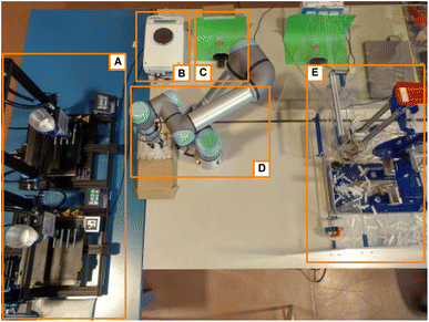

Fig. 1 Image of the experimental setup. (A) Two Direct3D pellet printers. (B) Analytical balance. (C) Camera vision station. (D) UR5 collaborative robot. (E) Automated Charpy impact test.

(A) Two Direct3D pellet printers: we use the Python library²⁶ to send the commands and get the status of the printers. To generate the gcode describing the necessary specimen we use the command line interface (CLI) version of and we change the needed parameters in the configuration file.²⁷ Once the gcode is generated, it is sent to a printer using and the process is monitored. We are printing the impact specimen in the on-edge position, which has 30 percent lower impact strength than the flat orientation¹⁷ while having a smaller contact area with the printer bed and taller sides, helping the robot to execute the removal of the specimen after the print. Between prints, the printer is cooled during the characterization process to reduce the degradation of the material in the heated barrel, and some amount is purged to discard the polymer that was already melted in the previous print. During printing, the distance between specimens helps cool down the layers naturally. Using two printers enables the parallelization of the printing process, which is the slowest part of the workflow and acts as a bottleneck.

(B) Gibertini CRYSTAL 500 CE analytical balance: it is used to weigh the samples after print to assess the under- and overextrusion common in low-quality prints. The balance is connected through an RS-232 port and USB adapter, and controlled with the library, which allows reading the measurements, taring and recalibrating from the script.

(C) Camera vision station: a Logitech C920 HD Pro Webcam is used to take pictures of the printed specimen placed in a custom-made fixed conical stand with a uniform background. The image quality is then analyzed in the way described in the following subsection.

(D) Collaborative robot (Universal Robots UR5 with OnRobot RG2 grippers): the robot picks the parts (i.e. material specimens) from the printing bed, moves the parts between stages comprising the workflow and operates scientific instruments where appropriate. When picking parts from the printer bed, the robot uses the integrated force feedback to accurately find the parts in the printing bed and perform a series of movements to lose them and pick them while it also detects anomalies (i.e. a part is missing, or is so strongly adhered that it is not possible to separate it from the printing bed). It is controlled by the library²⁸ for real-time control. This library provides functions to move the robot in different ways (linear, joint-based, etc.), feedback about position and force and an I/O interface to read and modify the digital inputs and outputs of the robot. Using a custom script for remote control allows the operation of the grippers with the I/O interface.

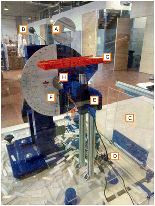
(E) Automated Charpy impact test (Fig. 2): a manual Zorn Stendal pendulum impact tester with a capacity of 4J is augmented to enable it to be operated by the collaborative robot in a fully automated way as outlined in the following paragraph.

Fig. 2 Automated Charpy impact test. (A): 4J pendulum. (B) Pendulum release lever. (C) Protective sliding door. (D) Arduino Uno microcontroller. (E) Logitech C920 HD Pro webcam. (F) Result dial in its initial position. (G) Hook tool. (H) Dial-resetting stepper motor.

Automated impact test. The working principle of this test is that a pendulum with known potential energy is released and breaks a standard specimen. The remaining energy after the impact is recorded by the movement of a needle. For safety, a transparent polymethyl methacrylate (PMMA) enclosure is constructed around the tester instrument, featuring a sliding door operated by a linear actuator. To facilitate automation, various components are integrated (Fig. 2), including custom 3D printed PLA parts and aluminum supports. A Logitech C920 HD Pro webcam and a stepper motor are mounted in line with the dial, and an arm on the motor pushes the dial to its initial position, detected by a limit switch. An Arduino Uno controls both the safety door and the dial arm, connected by a serial I/O interface to the workflow-governing Python script. Once the robot places the sample on the testing stand, the protective door is closed as a safety procedure, and moved along a rail by another stepper motor. After this motion, the robot arm drops the pendulum by pushing on the lever, accessible over the front panel of the safety enclosure, which is lower than the remaining sides. The resulting impact measurement is captured using camera vision from the analytical dial, and the stepper motor restores the dial to its initial state after each test. Subsequently, the door opens again, and the robot's grippers are used to slow down the pendulum, which is then brought back to the top and locked into place by the robot using a 3D-printed hook. The Charpy impact tests were carried out at room temperature and repeated four times for specimens printed simultaneously.

Camera vision is implemented using the images of the needle's initial and final positions after conducting the test. Subsequently, the absolute difference between these images is computed by subtracting one from the other. The resulting final image is then subjected to binarization. The positions of the dials are then recovered using Hough transform which allows for straight-line detection. Finally, the angle between the needle in its initial and final positions can be used to calculate the potential energy dissipated by the pendulum after impacting the sample. The relation between the angle and the latter is nonlinear but can be recovered through a prior one-time analysis of the dial's scale. All tasks related to the above image analysis are implemented using the OpenCV package.

By automating this test, we also expect an increased accuracy compared to human operation of the same test: by always measuring the result from the same camera position and resetting the needle to the same zero spot, we reduce the possibility of imprecisions.

Materials, specimens, and characterization

We demonstrate an application of the robotically automated workflow using two commercially available bio-based polylactide (PLA) grades obtained from NatureWorks, Ingeo 4043D and Ingeo 3251D with a melt flow index (MFI) of 6 g per 10 min and 80 g per 10 min, respectively. The corresponding samples were denoted as HPLA and LPLA for high molecular weight and low molecular weight, respectively. Both have densities of 1.24 g cc⁻¹. The material test specimens were printed directly from the commercially available pellets. For the impact test, four specimen samples with dimensions of 10 mm × 4 mm × 100 mm were printed. For the density measurement and quality assessment, three cylindrical specimen samples with 20 mm external diameter, 15.2 mm internal diameter and 20 mm height were printed. The printed parts can be seen in Fig. 3.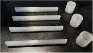

Fig. 3 Parts printed in each experiment. On the left, four rectangular samples for the impact test. On the right, three hollow cylinders for visual surface analysis.

Taking into account their volumes and densities, the expected weight for each of the printed parts at 100% infill can be calculated. However, the real weight depends on the printing parameters, so some printing parameters may cause under-extruded parts that have a weight lower than expected, caused by insufficient material being extruded and pockets of air being left between printing lines, while other parameters may cause over-extrusion, with more material extruded than the one needed and leading to an increase in the dimensions. This variation in the amount of material that conforms on the parts will have relevant effects on the mechanical properties of the printed objects, hence the importance of optimizing said parameters to have objects as close to the design as possible.

To quantify this, we define ΔW as the objective to maximize:

If a sample fails to print (because of adhesion issues or similar), only the properly printed ones will be taken into account. If none of them succeed, we assume that said parameters weren't suitable for printing and include them as ΔW = −1, meaning the worst possible result. Technically it would be possible to obtain even lower values than −1 if the measured weight is more than twice the expected weight, but this outcome has never been observed by us in the ranges of parameters that we have been considering. The use of an absolute value for the difference in weight is a simple way to calculate over- and under-extrusion in the same optimization process.

Four parameters are selected to be optimized (shown in Table 1): printing speed modifier (expressed as a percentage with respect to the standard one selected by the slicer), layer height, layer width and extrusion flow multiplier. The latter one is also expressed as a percentage, and its role is to transform the millimeters of filament to be extruded (determined by the slicer for a filament printer) into revolutions of the internal screw of the pellet printer. The initial value of 1000% was determined by extruding in air and selecting the flow rate after which a relatively constant flow of material is extruded. This parameter depends highly on the viscosity of the material, so it is possible that a more fluid material will need a much smaller multiplier and vice versa. While we used a restricted range for paper based on some prior experience, trying a material completely blindly would require trying a wider parameter range, further justifying the need for automation. The remaining parameters, such as extrusion temperature, bed temperature, etc., are kept constant between prints, as well as the 100% infill to make them adequate for mechanical testing.

Table 1 Parameters to optimize in the experiments

Parameter (units)	Min. value	Max. Value
Printing speed (%)	50	150
Extrusion flow (%)	1000	5000
Layer height (mm)	0.2	0.6
Layer width (mm)	0.6	1.0

---

Another property considered in this study is the surface quality of the 3D prints. Selecting appropriate printing parameters significantly influences the periodicity of the layers, the stability of extrusion, and the consistency of the sides of the printed cylindrical specimens. To address this, we conduct a study on the print quality of the samples using image processing techniques, analyzing significant changes in interlayer roughness between the layers of cylindrical specimens. The experimental setup employed will follow the configuration depicted in Fig. 1 (C).

The methodology employed for analyzing the 3D printing of the components within this framework is as follows: two photographs are captured, one before placing the cylinder on the stage and the other after placement. The absolute difference between the first and second images is calculated to highlight the printed cylinder introduced in the second photo. Subsequently, the result is binarized, and the contours of the identified objects are extracted using the and functions from the library. To prevent possible confusion with shadows, the silhouettes are then discriminated based on their size. After obtaining the silhouette of the cylinder, an algorithm is employed to detect the corners by analyzing the change of slope in the derivative at each point along the contour. This approach enables the determination of the inner diameter of the cylinder, which depends on the height at which it adheres to the cone, and identifies the contours of both the left and right sides of the cylinder, located between the top and bottom corners of the cylinder.

In order to assess the quality of the samples, we employ the roughness average (RA) as a measure, a commonly used parameter for quantifying surface roughness.²⁹ It represents the average variation of the surface profile from its primary profile or center line within a designated evaluation length. Primary profiles of the cylinders were calculated using a linear regression of the points corresponding to the different contours of the two sides. In this context, the RA serves as an indicator of the level of defects present on the sides of the cylinders and it's defined as:

where L is the evaluation length and x(y) is the height of the surface profile at location y, which corresponds to the X coordinate of the side contour at the Y coordinate measured from the primary line.

The arrangement of the parts on the stand, as well as the resolution of the camera, allows us to obtain images of the parts in which 1 pixel represents about 0.1 mm in reality. During the study, the height of the layer is one of the optimization parameters, varying between 0.2 mm and 0.6 mm and, therefore, the height in pixels of each layer will be represented by between 2 and 6 pixels. The resolution available is not sufficient to study the intralayer roughness variation, the interlayer distance being the one we are interested in to measure irregularities in the printing quality of the parts.

3D printing parameter sampling and optimization

In order to find the optimal printing parameters targeting the weight of the printed parts being as close as possible to the expected weight, we investigate two approaches, design of experiments (DOE) by Latin hypercube sampling (LHS)³⁰ and Bayesian optimization.

For LHS we use the implementation from the Python scipy statistical functions package. The statistical sampling method is considered to be among state-of-the-art DOE methods. It generates random samples of parameter values based on the Latin square design. LHS is especially widely used in Monte Carlo simulation to save computation time. We use non-orthogonal LHS sampling. This technique does not have a predefined number of sampling points, and there is no clear consensus about the ideal size. Articles like the one from Manache et al.³¹ review how different sources recommend different sample sizes, from as little as 4K/3 to 3K, with K being the number of dimensions. In our case, with 4 dimensions, 10 samples seemed like a reasonable compromise between accuracy and experimental cost.

For the Bayesian optimization implementation, we rely on the Python-based software tool, gpCAM,³² a tool for autonomous data acquisition and analysis. gpCAM has been developed for the complex field of materials science, a field that raises many challenges, such as vast parameter spaces and inhomogeneous measurement noise, involving applications with often significantly different length scales for different directions of the parameter space. gpCAM uses Gaussian processes (GPs) as a surrogate model. GPs highly depend on the kernel function and respective hyperparameters. In the case of gpCAM, we choose the default kernel, an anisotropic once differentiable 3/2 Matérn kernel. This results in d + 1 hyperparameters that need to be estimated, i.e. the signal variance and d length scale parameters (d denotes the dimension of the design space). We set the allowed range for the hyperparameters to be the same for all of them, i.e. a lower bound of 0.001 and an upper bound of 1000 and the initial guesses were chosen as the mean of the lower and upper bounds. For training of the GP, the maximum number of iterations before the optimization algorithm is terminated is set to 20. In order to determine where we observe the function next, we find the maximum of the so-called acquisition function. For balancing between exploitation and exploration, an upper-confidence-bound (UCB) acquisition function, i.e.

a(x;λ) = μ(x) + λσ(x)

is chosen, where μ(x) denotes the posterior mean and σ(x) the standard deviation or uncertainty of the function at point x with the trade-off parameter λ chosen here as λ = 1. For global optimization of the acquisition function, a genetic algorithm is used with a population size of 50. The rest of the parameters are maintained at the default values. We use the GPOptimizer class for training and optimization and implemented our own loop coupling it with our experimental robotic setup.

The LHS and BO approaches are tested in the previously described robotically automated setup. For the LHS setup, we feed in one point at a time from the ten previously calculated samples. In the case of BO we feed in one point at a time but after each step update the GP and find the next optimal point based on the maximal acquisition value.

Results and discussion

As seen in Fig. 5, 3D printing of the test specimens with arbitrary parameters may lead to very different results. The impact specimen A in this figure is suffering from underextrusion, as can be deduced from its reduced weight (ΔW = −0.31 ± 0.03) and its poor surface quality, with very irregular layers riddled with small holes or air bubbles. In contrast, the specimen shown in B has a much more similar weight to the expected one (ΔW = −0.02 ± 0.02), and a much more regular surface without so many imperfections. The difference between samples is not only aesthetic: sample A has a much lower impact strength (0.37 ± 0.09 J) compared to B (0.78 ± 0.03 J). This dramatic reduction of mechanical properties suggests that it is indispensable to find a systematic way to explore the parameter space (Table 2).

Table 2 Parameters and results for LPLA samples from Fig. 5

Parameter (units)	Sample A	Sample B
Printing speed (%)	65	145
Extrusion flow (%)	1200	2500
Layer height (mm)	0.46	0.42
Layer width (mm)	0.62	0.78
ΔW	−0.31 ± 0.03	−0.02 ± 0.02
Impact (J)	0.37 ± 0.09	0.78 ± 0.03

---

Aside from measuring the difference in weight and impact strength, the surface quality can be assessed by printing cylindrical shapes and evaluating their regularity using RA, as described in the Methods section. In Fig. 4, an example of two cylinders with different printing qualities is shown. The one with poor printing quality has RA = 0.148 mm and ΔW = −0.396, while the one with better quality has RA = 0.036 mm and a much smaller ΔW = −0.122. In this way, RA serves as an additional filter to identify parameters that lead to poor printing quality, and further validate the ones that are deemed optimal according to another criterion (e.g. ΔW and impact strength). On analyzing the available data, it is found that RA > 0.10 mm is a sensible threshold that allows the prints with bad quality for HPLA to be identified. However, LPLA has a higher fluidity and causes the printed layers to be inherently more irregular, so the RA > 0.10 mm threshold appears to be too restrictive and filters out too many prints with acceptable quality. Thus, for LPLA a threshold of RA > 0.15 mm is more fitted.

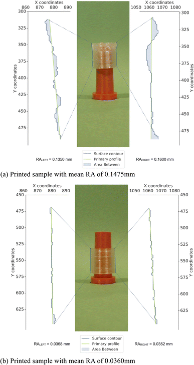Fig. 4 HPLA 3D printed cylinders showing (a) bad and (b) good surface quality based on the average RA calculated in their two sides.

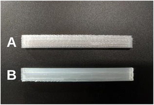Fig. 5 Examples of impact test samples with different qualities: under-extruded (A) and close to the ideal weight (B).

In Fig. 6, the relationship between weight fraction (the experimental weight divided by the expected weight) and impact strength is shown. There is a clear tendency for improvement of the mechanical properties with the increase in weight. Values of the weight fraction >1.0 mean overextrusion and exceed the dimensions of the sample, so the objective is to find parameters that allow the weight fraction to be as close to 1 as possible, maximizing ΔW.

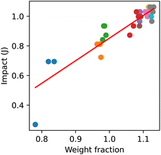Fig. 6 Correlation between the weight fraction and impact strength for HPLA. Different color group samples printed in the same experiment. R² = 0.82, MAE = 0.04.

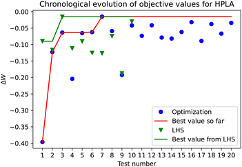
In Fig. 7, the results from Bayesian optimization for 20 experiments (blue points) and LHS for 10 experiments (green triangles) for HPLA, as described in the Methods section, are compared to their respective best objective value found. In the points sampled by LHS, a result with only 1.54% deviation from the expected weight can be found. BO provides a slight improvement (1.49% deviation) within the 20 experiments performed, suggesting that in this parameter space a LHS of 10 samples can be enough to find a reasonably good result, while BO can further improve this result and offer a more robust result. The performance of BO significantly depends on the choice of the surrogate model and the acquisition function. We chose an UCB acquisition function due to its track record but note that many acquisition functions are being investigated.³³ Another popular choice for autonomous experimentation is to first perform pure exploration by e.g. maximizing the posterior variance for several iterations and then switching to an exploitation-focused approach by using for instance an expected improvement acquisition function.¹⁸ The choice of the acquisition function has a significant impact on the choice of the next sampling point, and hence, it is important to the overall performance of Bayesian optimization. This aspect of our system will be further investigated in a future study.

Fig. 7 Results for 20 BO experiments (blue circles) and 10 LHS samples (green triangles) for HPLA. The red line shows the evolution of the best result found by BO, and the green line serves as a measure of the evolution of the LHS results. For BO, the best result is found on iteration 7, after which the algorithm balances exploration and exploitation.

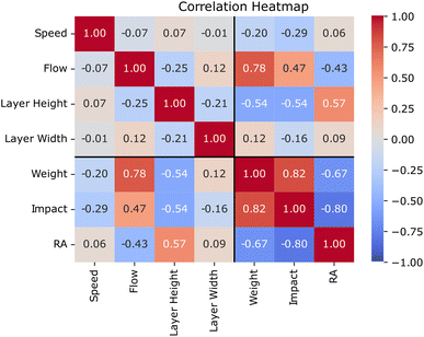
The importance of the parameters in the different tested properties is shown in Fig. 8. The three properties (ΔW, impact strength and RA as a measure of surface quality) show a clear correlation between them. Also, it is shown that the most relevant parameter is the extrusion flow, followed by the layer height, while the other parameters have little impact on the properties.

Fig. 8 Pearson correlation between the parameters (speed, flow and layer height and width) and properties (weight, impact and RA) for HPLA. Flow appears to be the most influential parameter for the results, followed by the layer height. The three properties are cross-correlated to each other.

From Fig. 7 one could assume that the algorithm is still exploring or still balancing between exploitation and exploration after the best point is found. Fig. 9 and 10 show the posterior mean, covariance and acquisition function for the flow and the layer height and the speed and layer width after 7 or 20 iterations, respectively, and confirm that there are still uncertain areas after 7 iterations but even after 20 iterations. The best point for all the dimensions is found in a certain area but sufficient data are not available for adequate hyperparameter estimation yet, and thus, the model does not capture the complexities of the design space yet. After 20 iterations, the best point for the less important dimensions, i.e. speed and layer height is found in a medium uncertain area. For the components of high importance, such as flow and layer height, the domain is already much more clearly defined. However, there is still some uncertain area left that lies in a different area than that of the optimal point. Nevertheless, after 20 iterations the balanced acquisition function clearly favors exploitation over exploration.

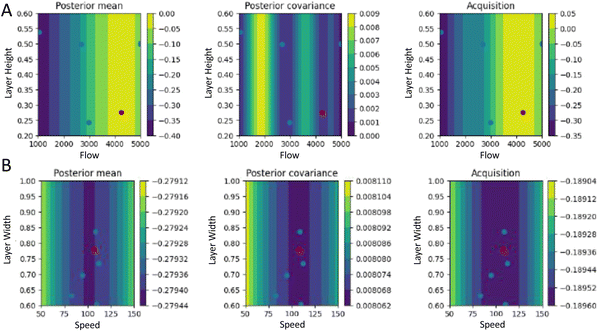Fig. 9 Contour plot of the posterior mean, covariance and acquisition function at iteration 7 corresponding to the experimental run shown in Fig. 7 for (A) the two most relevant parameters in this optimization (flow and layer height), and (B) the remaining parameters (speed and layer width). Here the current point (in red) is the one that minimizes the acquisition function. The previous samples are denoted by the blue points. The plots show the slices corresponding to the middle of the domain for the remaining 2 of the 4 dimensions.

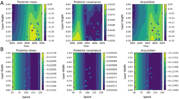Fig. 10 Contour plot of the posterior mean, covariance and acquisition function at iteration 20 corresponding to the ending of the experimental run shown in Fig. 7 for (A) the two most relevant parameters in this optimization (flow and layer height), and (B) the remaining parameters (speed and layer width). Here the current point (in red) is the one that minimizes the acquisition function. The previous samples are denoted by the blue points. The plots show the slices corresponding to the middle of the domain for the remaining 2 of the 4 dimensions.

Fig. 10 illustrates that the length scale parameters corresponding to the most important dimensions, i.e. the flow and the layer height, are estimated to be of the same order of magnitude as their scale. However, the other two dimensions, corresponding to the layer width and speed were estimated to be two to three orders of magnitude larger than their scale, and thus significantly overestimated. This further supports our observation in relation to Fig. 8 that the latter two parameters do not seem important when optimizing for weight. In ref. 18, for example, to avoid extreme values for the hyperparameters the authors limit them to not differ less or more than a factor of 10 from their respective initial values during the optimization process. Similar considerations to avoid extreme values for the hyperparameters or adjusting the allowed ranges for the hyperparameters could further improve the results. In general, small datasets make the estimation of the hyperparameters challenging. Given that more data are available, one could also estimate the noise as one to multiple additional hyperparameters from the maximum likelihood or estimate it from more experimental data to achieve better performance.

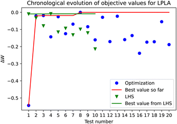
For LPLA, the optimization-based approach finds the best design after eight iterations (Fig. 11). In the LHS design, there are two points that are just slightly below this point, also under 1% deviation. The optimization is still focused on exploration for the course of all the 20 experiments, suggesting that it has not found yet a model with enough confidence. This may have different explanations; either some of the dimensions are not important for the optimized property and/or the space is much more complex in general and we need significantly more samples and/or there is remarkably more measurement noise present for this material than for HPLA. By default, gpCAM uses a constant measurement noise of 1% of the mean of the output values, in our case the ΔW values, such that the noise for the LPLA material may be significantly underestimated.

Fig. 11 Results for 20 BO experiments (blue circles) and 10 LHS samples (green triangles) for HPLA. The red line shows the evolution of the best result found by BO. For BO, the best result is found on iteration 8, but the algorithm continues exploring without finding some stability region.

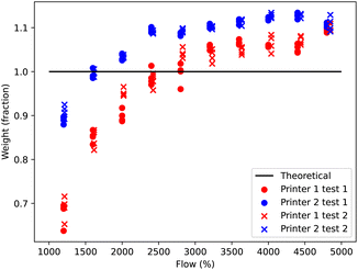
Running several tests using the LHS configuration parameters on multiple printers of the same model results in different values of ΔW for the same parameters. These tests confirm that there is a significant amount of noise present (up to 3% within the same printer, up to 11% between printers), as can be seen in Fig. 12.

Fig. 12 Tests of LPLA LHS in multiple printers (printer 1 in red, printer 2 in blue, dots for test 1, and crosses for test 2) of the same kind to test the reliability of the results. A consistent difference can be seen between printers.

Recent studies³⁴ showed that the best way to incorporate inhomogeneous noise would be to estimate the noise during the collection of samples especially with respect to aiming for autonomous experimentation. The authors found that assuming fixed noise may result in ineffective autonomous experiments. Hence, to ensure that our autonomous experimentation setup results in optimal design parameters while performing the least possible number of autonomous experiments, we would need to collect significantly more data for each material and printer beforehand or on the go which was out of scope in the course of this study.

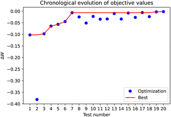
As the variation in ΔW seems to be caused mainly by the use of several printers, it seems that the proper way to get more consistent values that allow an optimization process is to use only one printer during the said process. Such an optimization that involved only one 3D printer is shown in Fig. 13, where the values for ΔW improve with iteration time until reaching an optimum, after which the algorithm is mainly exploiting the area. Our experience indicates that our setup faces a fragile balance between the throughput determined by the number of parallel printers involved and the length of experimental campaigns necessary to collect enough data points to address adequate noise and hyperparameter estimation. We plan to investigate this balance in future studies.

Fig. 13 Bayesian optimization of LPLA with a single printer for 20 experiments. The red line shows the best value so far. The results keep improving throughout the experimental run, suggesting that the algorithm is focused on exploiting a region with good results.

Studies like ref. 18 use multiple filament 3D printers working in parallel to greatly increase the throughput. However, pellet 3D printing is a less developed technology that still lacks the reliability of the filament one. We believe that the variability in results may come from the internal state of the molten material inside the different printers, and it is not comparable to experiments made with commercial filaments in more standard printers. Thus, the conclusions regarding the effect of using a single printer or several working in parallel are specific to our setup.

Conclusions

In this contribution, we have aimed to facilitate the development of new thermoplastic polymer materials by the introduction of a MAP focused on the manufacturing and testing of material specimens. Specifically, we have presented an automated workflow that can take polymer pellets as the input, identify 3D printing parameters to produce quality specimens and perform their mechanical property testing via a Charpy impact test. The workflow involves pellet-based 3D printers working in parallel, a collaborative robot manipulator to handle the printed specimen, a balance and camera vision system to monitor the quality of the specimen, and an analog impact tester instrument, the operation of which has been fully automated with the aid of robot and do-it-yourself accessories. We have demonstrated the automated setup using two grades of bio-based PLA material. We considered four parameters that control the print quality: printing speed modifier, layer height, layer width and extrusion flow multiplier. The flow multiplier was proved to be the parameter with higher relevance in the resulting samples, followed by the layer height. Our study has explored two approaches to identify printing parameters leading to high-quality samples. Our results indicate that reasonably high-quality 3D print parameters can be identified from within 10 print experiments selected using the Latin hypercube sampling approach, with a smaller deviation from the theoretical value than the experimental error present, which is around 1% in the best cases. Further improvement can be reached using the BO approach. However, this approach requires a careful selection of the design problem and an adequate estimation of noise and other hyperparameters. The latter may require an overwhelming number of experiments to be addressed. In addition, further improvements could be achieved by considering other acquisition functions and surrogate models. We assumed that the significant amount of noise present caused the major issues. Hence, we suggested a mitigation strategy based on implementing each optimization process in a single 3D printer to limit the variation between prints and demonstrated that such a strategy indeed performs as expected.

Data availability

The data that were used to generate the figures presented in the manuscript and examples of the code for running Bayesian Optimization are attached as ESI File.† There are no other datasets related to the manuscript.

Author contributions

M. HdV. developed and tested the presented robotic setup (incl. both software and hardware integration). C. S. contributed the software for the search of optimal 3D print parameters. L. E.-P. developed the computer vision methodology and software. E. D.-L. and J. I.-Z. contributed to the development of an automated Charpy instrument. B. O. and D.-Y. W. helped with the material selection and processing as well as the validation of the presented setup. M. H. conceptualized and supervised the project. All authors contributed to the writing and revising of the manuscript.

Conflicts of interest

There are no conflicts to declare.

Acknowledgements

We acknowledge the support from the “(MAD2D-CM)-IMDEA Materials” project funded by Comunidad de Madrid, the Recovery, Transformation and Resilience Plan, and NextGenerationEU from the European Union. We wish to thank Marcus Noack and Paolo Legnani for their helpful suggestions on setting up gpCAM software and pellet printing, respectively. Additionally, we thank one of the reviewers for providing constructive feedback on hyperparameters involved in the implementation of Bayesian optimization.

Notes and references

1. M. Biron, Material Selection for Themroplastic Parts, William Andrew Applied Science Publishers, Chichester, 1st edn, 2016.
2. R. Banerjee and S. Ray, Polym. Eng. Sci., 2021, 61, 617–649.
3. J.-M. Raquez, Y. Habibi, M. Murariu and P. Dubois, Prog. Polym. Sci., 2013, 38, 1504–1542.
4. L.-T. Lim, R. Auras and M. Rubino, Prog. Polym. Sci., 2008, 33, 820–852.
5. M. M. Flores-Leonar, L. M. Mejía-Mendoza, A. Aguilar-Granda, B. Sanchez-Lengeling, H. Tribukait, C. Amador-Bedolla and A. Aspuru-Guzik, Curr. Opin. Green Sustainable Chem., 2020, 25, 100370.
6. F. Häse, L. M. Roch and A. Aspuru-Guzik, Trends Chem., 2019, 1, 282–291.
7. N. Science and T. C. (US), Materials genome initiative for global competitiveness, Executive Office of the President, National Science and Technology Council, 2011.
8. F. Delgado-Licona and M. Abolhasani, Adv. Intell. Syst., 2023, 5, 2200331.
9. B. Burger, P. M. Maffettone, V. V. Gusev, C. M. Aitchison, Y. Bai, X. Wang, X. Li, B. M. Alston, B. Li and R. Clowes, et al. , Nature, 2020, 583, 237–241.
10. B. P. MacLeod, F. G. Parlane, T. D. Morrissey, F. Häse, L. M. Roch, K. E. Dettelbach, R. Moreira, L. P. Yunker, M. B. Rooney and J. R. Deeth, et al. , Sci. Adv., 2020, 6, eaaz8867.
11. L. M. Roch, F. Häse, C. Kreisbeck, T. Tamayo-Mendoza, L. P. Yunker, J. E. Hein and A. Aspuru-Guzik, Sci. Robot., 2018, 3, eaat5559.
12. M. B. Rooney, B. P. MacLeod, R. Oldford, Z. J. Thompson, K. L. White, J. Tungjunyatham, B. J. Stankiewicz and C. P. Berlinguette, Digital Discovery, 2022, 1, 382–389.
13. X. Wang, M. Jiang, Z. Zhou, J. Gou and D. Hui, Composites, Part B, 2017, 110, 442–458.
14. G. Spinelli, P. Lamberti, V. Tucci, R. Ivanova, S. Tabakova, E. Ivanov, R. Kotsilkova, S. Cimmino, R. Di Maio and C. Silvestre, Composites, Part B, 2019, 167, 467–476.
15. Y. Zhang and S. K. Moon, J. Comput. Des. Eng., 2021, 8, 489–509.
16. M. Á. Caminero, J. M. Chacón, E. García-Plaza, P. J. Núñez, J. M. Reverte and J. P. Becar, Polymers, 2019, 11, 799.
17. E. García, P. Núñez, J. Chacón, M. Caminero and S. Kamarthi, Polym. Test., 2020, 91, 106860.
18. A. E. Gongora, B. Xu, W. Perry, C. Okoye, P. Riley, K. G. Reyes, E. F. Morgan and K. A. Brown, Sci. Adv., 2020, 6, eaaz1708.
19. A. E. Gongora, K. L. Snapp, E. Whiting, P. Riley, K. G. Reyes, E. F. Morgan and K. A. Brown, Iscience, 2021, 24, 102262.
20. J. R. Deneault, J. Chang, J. Myung, D. Hooper, A. Armstrong, M. Pitt and B. Maruyama, MRS Bull., 2021, 46, 566–575.
21. S. Jin, J. R. Deneault, B. Maruyama and Y. Ding, Proceedings of the International Symposium on Flexible Automation 2022 International Symposium on Flexible Automation, 2022, pp. 173–179.
22. T. Erps, M. Foshey, M. K. Luković, W. Shou, H. H. Goetzke, H. Dietsch, K. Stoll, B. von Vacano and W. Matusik, Sci. Adv., 2021, 7, eabf7435.
23. G. S. Ganitano, S. G. Wallace, B. Maruyama and G. L. Peterson, Prog. Addit. Manuf., 2023, 1–11.
24. Z. Jin, Z. Zhang, K. Demir and G. X. Gu, Matter, 2020, 3, 1541–1556.
25. Y. Shaik, J. Schuster and A. Shaik, Open Access Libr., 2021, 8, e7698.
26. K. Yanev, G. Seguin, et al., Printrun entry in pypi.org, available online: https://pypi.org/project/Printrun/, accessed: 2023-07-25.
27. J. Prusa, et al., Prusaslicer CLI repository in github, available online: https://github.com/prusa3d/PrusaSlicer/wiki/Command-Line-Interface, accessed: 2023-07-25.
28. A. P. Lindvig, UR-RTDE entry in pypi.org, available online: https://pypi.org/project/ur-rtde/, accessed: 2023-07-25.
29. D. Whitehouse, Surfaces and their Measurement, Elsevier, 1st edn, 2012.
30. M. D. McKay, R. J. Beckman and W. J. Conover, Technometrics, 1979, 21, 239–245.
31. G. Manache and C. Melching, Proceedings of the 32nd Congress of the International Association of Hydraulic Engineering and Research, 1–6 July 2007, Venice, Italy, 2007.
32. M. M. Noack, G. S. Doerk, R. Li, J. K. Streit, R. A. Vaia, K. G.Yager and M. Fukuto, Sci. Rep., 2020, 10, 17663.
33. X. Wang, Y. Jin, S. Schmitt and M. Olhofer, ACM Comput. Surv., 2023, 55, 1–36.
34. M. M. Noack and K. G. Reyes, MRS Bull., 2023, 48, 153–163.

---

Footnote

† Electronic supplementary information (ESI) available. See DOI: https://doi.org/10.1039/d3dd00141e

---