
 Open Access Article
 This Open Access Article is licensed under a
 Creative Commons Attribution 3.0 Unported Licence
Towards the automated extraction of structural information from X-ray absorption spectra†
Tudur
David
*a,
Nik Khadijah
Nik Aznan
b,
Kathryn
Garside
b and
Thomas
Penfold
 a
a
aChemistry, School of Natural and Environmental Sciences, Newcastle University, Newcastle upon Tyne, NE1 7RU, UK. E-mail: tom.penfold@newcastle.ac.uk
bResearch Software Engineering Group, Catalyst Building, Newcastle University, Newcastle upon Tyne, NE1 7RU, UK
First published on 29th August 2023
Abstract
X-ray absorption near-edge structure (XANES) spectroscopy is widely used across the natural sciences to obtain element specific atomic scale insight into the structure of matter. However, despite its increasing use owing to the proliferation of high-brilliance third- and fourth-generation light sources such as synchrotrons and X-ray free-electron lasers, decoding the wealth of information encoded within each spectra can sometimes be challenging and often requires detailed calculations. In this article we introduce a supervised machine learning method which aims at directly extracting structural information from a XANES spectrum. Using a convolutional neural network, trained using theoretical data, our approach performs this direct translation of spectral information and achieves a median error in first coordination shell bond-lengths of 0.1 Å, when applied to experimental spectra. By combining this with the bootstrap resampling approach, our network is also able to quantify the uncertainty expected, providing non-experts with a metric for the reliability of each prediction. This work sets the foundation for future work in delivering techniques that can accurately quantify structural information directly from XANES spectra.
1 Introduction
X-ray absorption spectroscopy (XAS) is a powerful tool for element specific investigation of the local geometric and electronic structure of molecules and materials in a broad range of different environments and under challenging operating conditions, e.g. in operando measurements of batteries and femtosecond time-resolved studies.1,2 For a particular absorption edge, a spectrum is usually split into two regions, the X-ray absorption near-edge structure (XANES) and extended X-ray absorption fine structure (EXAFS) region. The latter begins >50 eV above the edge and exhibits a distinct oscillatory behaviour associated with the interferences of the photoelectron wave from the absorbing atom with the wave scattered back from the neighbouring atoms. Consequently, it delivers information about coordination numbers and the bond distances for the first coordination shell to the absorbing atom. Usually the first step towards obtaining a quantitative description of the structure is achieved using a Fourier transform (FT) or wavelet transforms of the EXAFS signal, which yields a pseudo-radial distribution.3,4In contrast, at low photoelectron energies (<50 eV above the edge) associated with the XANES region, spectral features arise from the interference of scattering pathways between multiple atoms and therefore this region contains information about the three-dimensional structure usually within ∼6 Å of the absorbing atom.5 Qualitative insight from these spectra can be obtained using empirical rules, such as shifts in the absorption edge with oxidation state,6 changes in structural symmetry reflected in the pre-edge7,8 or shifts in above-ionisation resonances which can reflect bond length changes (Natoli's rule).9 However, quantitative decoding of the high information content within XANES spectra usually requires detailed theoretical calculations,10 and therefore unlike FT-EXAFS, there is no direct way of extracting structural insight from a spectrum.
To address the challenges associated with the analysis of XANES spectra, there has recently been a substantial research effort seeking to exploit supervised machine-learning/deep learning algorithms to predict spectral shape from an input structure or property.10–14 This, so-called forward mapping approach is akin to the approach used in a first-principles calculations, i.e. an input structure is used to solve the electronic Schrödinger equation and compute a particular spectrum, which is subsequently compared to the experiment one is trying to analyse. However, in terms of the interpretation of experimental spectra the reverse mapping problem, i.e. converting a spectrum into a property/structure, is in many ways the more natural, as it has the direct connection to the focus of the analysis, i.e. what structural information is contained within the spectrum?
Towards achieving this, Timoshenko et al. applied a multi-layer perceptron (MLP) model to identify the average size, shape, and morphology of platinum nanoparticles. The network was trained using theoretical XANES data, calculated with FEFF and FDMNES, but subsequently successfully applied it to interpret experimental spectra. The authors have extended this work to other related areas15–18 and while the results are very encouraging, they are always system-specific or restricted to a narrow class of systems. Consequently a new set of theoretical calculations and model would be necessitated for it to be applied to a different system.
In contrast, Carbone et al.19 used an MLP and convolutional neural network (CNN) to classify the local coordination environment around an absorbing atom from K-edge XANES spectra across each of the first row transition metals. They demonstrated that both these approaches were able to classify, with ∼86% accuracy, the symmetry of coordination environment from a spectrum. In addition, they showed that for octahedral and tetrahedral complexes, this could be largely achieved using only the pre-edge region of the spectrum, which is well-known to be important in determining the coordination geometry around the absorbing atom.7 Torrisi et al.20 extended this work using a random forest model to extract coordination numbers, average first coordination shell bond lengths and atomic charge of the absorbing atom. However, although both works demonstrate highly effective networks, both were trained and applied entirely on theoretical data; which does not address the true purpose of these networks, which would involve application to experimental data.
These previous works have largely focused upon classification models, translating spectra into structural properties such as coordination numbers. In contrast, Kiyohara et al.21 and Higashi et al.22 have both implemented MLP-based approaches to convert calculated XANES spectra into radial distribution functions at the oxygen K-edge. In contrast, in this work we implement a CNN that converts a given spectrum into a pseudo-radial distribution function, based upon the 2-body terms in the weighted atom-centered symmetry function (wACSF) descriptor. We demonstrate and explain its performance based upon simulated and experimental iron K-edge data. We show that our approach achieves a median error in first coordination shell bond-lengths of 0.1 Å, when applied to experimental spectra. In addition, by combining this with the bootstrap resampling approach, our network is also able to quantify the uncertainty expected providing non-experts with a metric for the reliability of each prediction. Finally, we discuss limitations of the present model and proposed ways in which this can be developed in future work.
2 Computational and technical details
2.1 Network details
The architecture of our deep neural network (DNN) is based upon a CNN and is shown schematically in Fig. 1. The network passes discretised Fe K-edge spectra through three 1D convolutional layers, each of which convolves the spectra with its own set of 2 filters. The kernel size is fixed to 8 and the stride for the cross-correlation is 2. The output of these convolutional layers is passed into an MLP, containing two hidden layers and an output layer. All layers are dense, i.e. fully connected, and each hidden layer performs a nonlinear transformation using the rectified linear unit (ReLU) activation function. The first hidden layer has a dimension of 256 and the subsequent layer is 128. The output layer comprises 50 neurons from which the discretised wACSF descriptor (see Section 2.2) is retrieved after regression. The filters and internal weights are optimised via iterative feed-forward and backpropagation cycles to minimise the empirical loss, defined as the mean-squared error (MSE) between the predicted, Gpredicted2, and calculated, Gcalculated2, descriptor (see Section 2.2) over the reference dataset.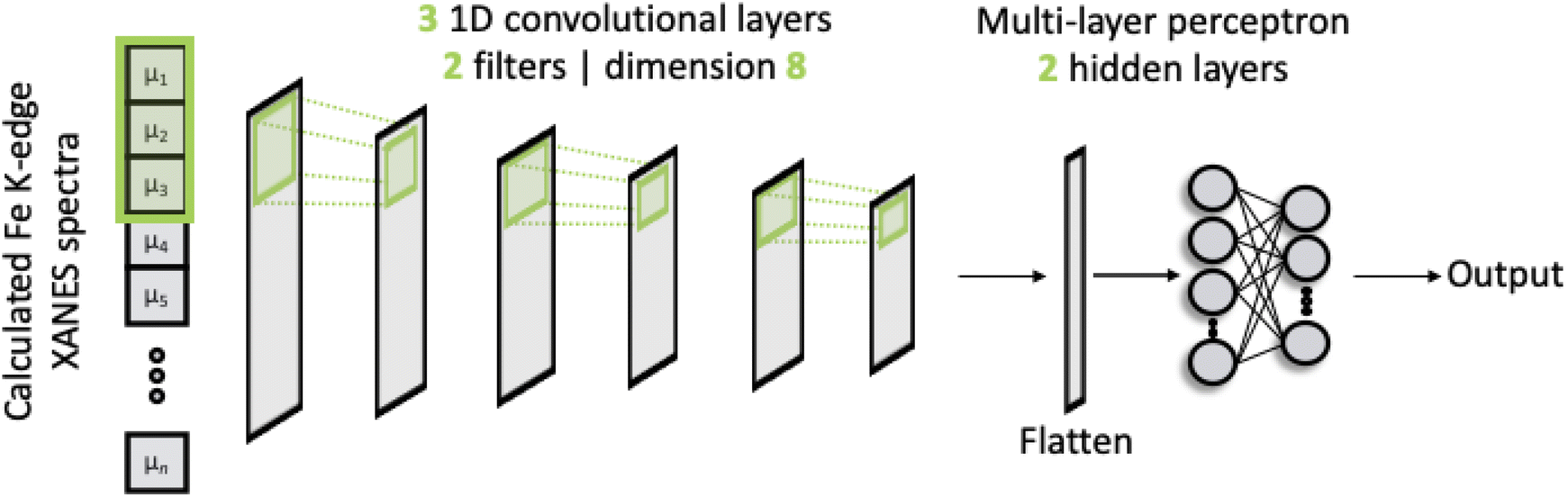 | ||
| Fig. 1 A schematic of the convolutional neural network used in this work. The network feeds discretised Fe K-edge spectra through three 1D convolutional layers. The output from these convolutional layers is passed into a multi-layer perceptron model. The filters and internal weights are optimised via iterative feed-forward and backpropagation cycles to minimise the mean-squared error between the predicted, Gpredicted2, and calculated, Gcalculated2, descriptor. | ||
Gradients of the empirical loss with respect to the internal weights were estimated over mini-batches of 32 samples and updated iteratively according to the Adaptive Moment Estimation (ADAM)23 algorithm. The learning rate was set to 2 × 10⁻³. The internal weights were initially set according to ref. 24. Unless explicitly stated in this article, optimisation was carried out over 50 iterative cycles through the network, commonly termed epochs.
The DNN is programmed in Python 3 with Pytorch.25 The Atomic Simulation Environment26 (ASE) API is used to handle and manipulate molecular structures. The code is publicly available under the GNU Public License (GPLv3) on GitLab.27
2.2 Featurisation
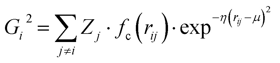
Atomic structures with many atoms contain more information than represented within a single spectrum and therefore extracting the full three dimensional Cartesian coordinates from a spectrum is an underdetermined problem. Our objective within the present work is to achieve an automated structural analysis comparable to FT-EXAFS, i.e. a pseudo-radial distribution function of atomic distances from the absorbing atom.Consequently, we focus upon converting the spectra into the two-body G2 terms of the weighted atom-centered symmetry function (wACSF) descriptor of Gastegger and Marquetand et al.,28 which encodes the local environments around X-ray absorption sites by dimensionality reduction. This descriptor has previously been used in the reverse problem, i.e. converting atomic structures into spectra13,14 and its use in the present work, opposed to a simple radial distribution function, is motiviated by future objectives of achieving cyclic consistency between the two models. The G2 terms take the form:
 | (1) |
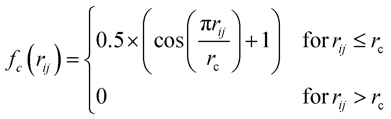 | (2) |
The radial distance, rc, supplied to fc has to be sufficiently large to include an appropriate number of nearest neighbours. From the perspective of an absorbing atom in X-ray spectroscopy, rc has to reflect the maximum cutoff distance to which XANES is sensitive and therefore we have used rc = 6.0 Å throughout. Throughout this work, we adopt an input feature vector containing 50G2 functions, constructed according to the “shifted” scheme.13
We note that previous work has transformed XANES spectra directly into radial distribution functions,21,22 rather than wACSF used here. The main difference between the two will be the weighting of contributions in the G2 wACSF by atomic number. This is consistent with physical processes responsible for the features in XANES spectra as different elements will exhibit different backscattering amplitudes and consequently a distinction between atomic contributions is advantageous. We also retain a wACSF descriptor here to consistent with previous work mapping the forward problem, i.e. structure to spectrum.13
2.3 Dataset
Our reference dataset, available at ref. 29, contains 36![[thin space (1/6-em)]](https://www.rsc.org/images/entities/char_2009.gif) 657 spectra–structure pairs developed structures extracted from the Cambridge Structural Database (CSD). This dataset incorporates 77 of the elements from the periodic table and molecules with a coordination number, defined as the number of atoms within 2.5 Å of the absorbing atom, between 2 and 16. The Fe K-edge XANES spectra (“labels”) for these structures were calculated using multiple-scattering theory (MST) within the muffin-tin approximation as implemented in the FEFF30 package. The calculations used a self-consistent potential and full multiple scattering up to a radius of 6 Å around the absorbing atom. After calculations, the absorption cross-sections were resampled via interpolation into 475 points over an energy range of 7112.5–7160 eV. Throughout, unless otherwise stated, the training and validation subsets were constructed “on-the-fly” throughout via repeated K-fold cross validation with five repeats and five folds, i.e. a five-times-repeated 80:20 split.
657 spectra–structure pairs developed structures extracted from the Cambridge Structural Database (CSD). This dataset incorporates 77 of the elements from the periodic table and molecules with a coordination number, defined as the number of atoms within 2.5 Å of the absorbing atom, between 2 and 16. The Fe K-edge XANES spectra (“labels”) for these structures were calculated using multiple-scattering theory (MST) within the muffin-tin approximation as implemented in the FEFF30 package. The calculations used a self-consistent potential and full multiple scattering up to a radius of 6 Å around the absorbing atom. After calculations, the absorption cross-sections were resampled via interpolation into 475 points over an energy range of 7112.5–7160 eV. Throughout, unless otherwise stated, the training and validation subsets were constructed “on-the-fly” throughout via repeated K-fold cross validation with five repeats and five folds, i.e. a five-times-repeated 80:20 split.
Fig. 2a shows a plot of the first two t-distributed stochastic neighbour embedding (t-SNE) components of the wACSF descriptor encoding each local geometry against the first t-SNE component of the spectra (colour bar). In contrast to the more commonly-used linear dimensionality reduction approach of principal component analysis (PCA), t-SNE is a non-linear approach which seeks to preserve the local structure of data by minimising the Kullback–Leibler (KL) divergence between distributions with respect to the locations of the points in the map. t-SNE is not a black box, but instead requires user-defined hyperparameters: the perplexity, learning rate, and the number of iterations which, to produce Fig. 2a, were set to 50, 60, and 1000, respectively. This shows well defined regions of correlation between the structural and spectra t-SNE, which makes the dataset amenable to learning. Fig. 2b shows the same t-SNE plot as Fig. 2a, but in this case the colours present a pseudo-coordination number, i.e. the number of atoms within 2.5 Å of the absorbing atom. This highlights that this pseudo-coordination number represents a significant factor determining the t-SNE data distribution show in Fig. 2a. The peach coloured region in Fig. 2a, which does not appear in Fig. 2b (i.e. not directly associated with coordination number), is associated with complexes exhibiting multiple absorbers and a strong presence of linear bonds, such as CO and CN, which strongly modulate the shape of the XANES spectrum.31
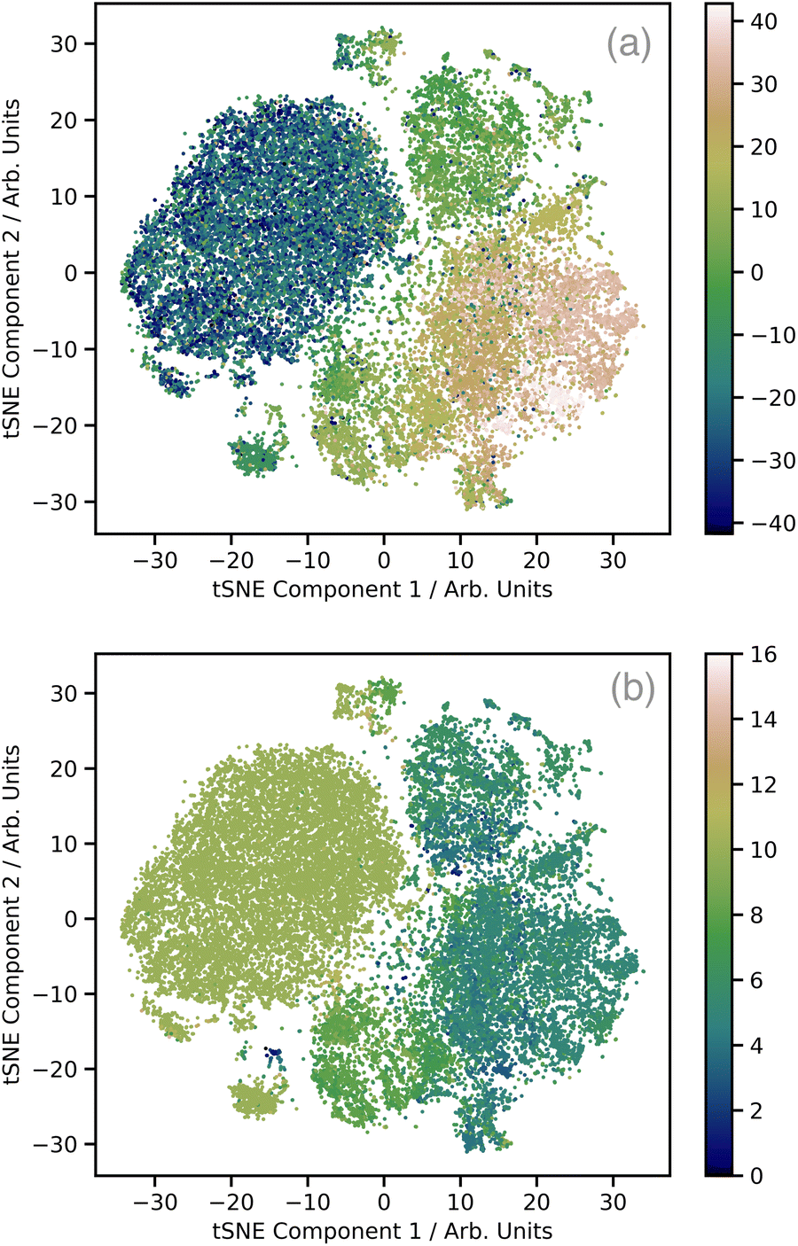 | ||
| Fig. 2 t-distributed stochastic neighbour embedding (t-SNE) analysis of the training set (a). The two axis are the first two components of the wACSF descriptor encoding each local geometry, while the colours represent the first t-SNE component of the spectra. (b) The same t-SNE plot as (a), but in this case the colours represent a pseudo-coordination number, i.e. the number of atoms within 2.5 Å of the absorbing atom. | ||
2.4 Bootstrap resampling
We have recently demonstrated that the bootstrap resampling technique can be used to estimate the uncertainty arising from neural network predictions of XANES spectral shapes from input structures.32 Here, we adopt the same approach estimating the uncertainty in the estimated structural predictions. Briefly, N machine learning models are optimised using N reference datasets sampled with replacement from the original reference dataset; each one of these is the same size as the original reference dataset and, consequently, may contain repeated instances of the same sample.33N independent instances of the machine learning model optimised using N bootstrapped reference datasets are then used to produce N independent predictions from which a mean prediction and standard deviation for each sample can be derived. Throughout this work N = 15.3 Results
Now we shift our focus to the results and analysis, which can be categorised as follows: firstly, we showcase the network's performance using theoretical training sets, evaluating its functionality and its capacity to predict uncertainty. Following that, we assess the network's performance when applied to experimental data.3.1 Network performance assessed using theoretical data
Fig. S1† shows the convergence of our DNN as a function of the number of forward passes through the dataset, commonly termed epochs. This shows that it is possible to optimise our DNN to effective convergence in 50 epochs, which will now be used through the remainder of this work. Fig. 3 shows the convergence as a function of the number of spectra used during the training process. Initially the MSE shows a rapid decrease during the first ∼15000 samples, followed by a more gradual improvement for the next 20000 samples. The remaining slow decline, indicates that convergence is not entirely achieved and suggests that there is still scope to improve further on the results communicated here by growing/optimising the dataset. However, the changes are small as chemical space is well represented and therefore more targeted strategies are required to identify the areas of improvement.
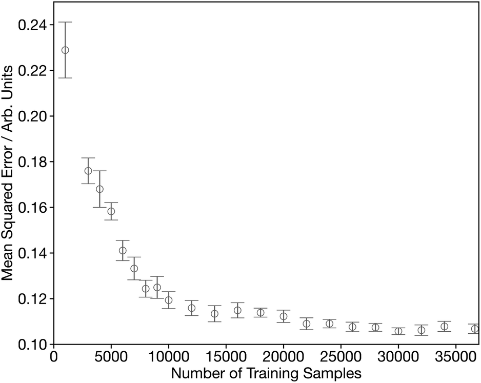 | ||
| Fig. 3 Learning curve showing the performance of the network, assessed by from five-times-repeated five-fold cross-validation, as a function of the number of training samples. | ||
Fig. 4a shows a histogram of the MSE for the 3500 spectra in the held-out dataset, composed entirely of theoretical spectra.29 The value of MSE alone can be misleading and therefore to add context, Fig. 4b–d show example theoretical (black) and predicted (grey) G2 wACSF with MSE of 0.004, 0.1, and 0.72 (see grey dashed lines in Fig. 4a). The spectrum with the median error of 0.1 is represented in Fig. 4c and corresponds to the material DALYOG. The G2 wACSF predicted with this error typically exhibits the correct shape and the error is predominantly associated in the prediction of the intensity of the peaks. The mean error for this held-out data set is 0.2, slightly larger than the median, being more sensitive than the median to the worst predictions, e.g. MIGDAT. The coefficient of variation (Cv) for these held-out predictions is 1.73, indicating, consistent with the histogram, a relatively small variability of points which are typically placed towards the higher-performance end.
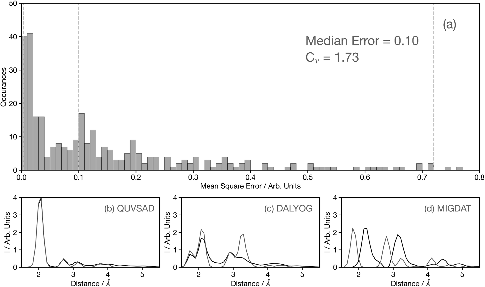 | ||
| Fig. 4 (a) Histogram of the MSE for the held-out data set predicted using the convolutional neural network model developed using the full training set and 50 epochs. The median error and coefficient of variation (Cv) are shown inset. To aid interpretation, the lower panels (b), (c), and (d) show example theoretical (black) and predicted (grey) G2 wACSF with MSEs of 0.004, 0.1, and 0.72, respectively. These are examples from the 0th–10th percentiles, 45th–55th percentiles (median) and 90th–100th percentiles, respectively, when the held-out dataset is ranked by MSE. The six-letter codes in panels (b), (c), and (d) are the Cambridge Structural Database identifiers of the samples presented. | ||
The peaks in the G2 wACSF shown in Fig. 4b–d indicate atomic distances from the absorbing atom and therefore are most important in terms of assessing the accuracy of the predictions. In the subsequent analysis, we quantify the accuracy of peak predictions generated by the network in two regions: close proximity to the absorber (1–3.5 Å) and far away from the absorber (3.5–6 Å). Close to the absorbing atom, the median and mean errors in the peak position are 0 Å and 0.07 Å, respectively. In the latter case, considering the utilization of 50G2 functions across a range of 5.0 Å, the error is equivalent to the grid point spacing. The interquartile range for peak position errors is 0.1 Å, indicating that overall there is high accuracy in the predictions for this region of the G2 wACSF. In the region further from the absorbing atom, the median and mean error increases to 0.2 Å and 0.22 Å, respectively. The interquartile range is 0.2 Å. This observed increase in error is expected, because as illustrated in Fig. 4b–d, this region exhibits lower intensities compared to the vicinity of the absorbing atom. Consequently, during the model refinement, even if the description is inadequate, it will result in much smaller MSE. However, despite this, an error of approximately ∼0.2 Å is still considered acceptable for this distant region of the G2 wACSF.
Having established the performance of the network, in the following we seek to assess the factors influencing the predictions made by the network, with a particular focus on factors that may influence the performance when applying the trained network to experimental data. Theoretical predictions of absolute transition energies are often challenging34 and consequently, Fig. 5 shows the effect on the G2 wACSF predictions when a constant energy shift of 1.0 and 2.0 eV is applied to the calculated spectra for VELFEX and ATOFEW. The former is in the top 10% of predictions shown in Fig. 4, while ATOFEW is in the bottom 10%. Fig. 5 shows that the spectral shift does not have a strong effect on the peak positions in either, but clearly is larger for ATOFEW, especially in terms of G2 wACSF intensities. Fig. S2† shows a similar case, but instead the spectra chosen exhibit more distinct intensity changes. In this case, for the spectrum which yields an accurate G2 wACSF prediction (XABHIU) the changes are larger than observed in Fig. 5 for VELFEX, but remains much smaller than PIFNUO, which offers a poor prediction of G2 wACSF which is also strongly sensitive to spectral shifts.
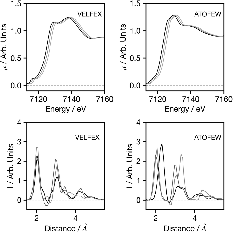 | ||
| Fig. 5 Spectra (upper) and G2 wACSF (lower) as a function of spectral shift. Black: original spectrum, dark grey: 1.0 eV shift, grey: 2.0 eV shift. The six-letter codes are the Cambridge Structural Database identifiers upon which the original spectra are based. | ||
Fig. 6 shows the influence of resolution, with spectra increasingly broadened using a Gaussian function with a full width at half maximum (FWHM) between 0.5 and 3 eV. Overall for both spectra, and for the spectra showing more prominent features (Fig. S3†), the broadening has very limited influence on the G2 wACSF prediction. Similar to the example for spectral shifts, it is evident that the largest changes are observed in the cases when the original spectrum provides a poor prediction of the structure (in terms of MSE) when compared to the expected G2 wACSF. This implies that when the network's performance is subpar, it becomes more susceptible to variations in absolute energy and spectral resolution, thus presenting a potential metric that can be utilised to evaluate confidence in predictions.
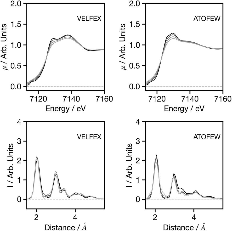 | ||
| Fig. 6 Spectra (upper) and G2 wACSF (lower) as a function of spectral broadening. Black: original spectrum, dark grey: 0.5 eV additional Gaussian broadening, grey: 1.0 eV additional Gaussian broadening and light grey: 3.0 eV additional Gaussian broadening. The six-letter codes are the Cambridge Structural Database identifiers upon which the original spectra are based. | ||
Fig. 7 seeks to assess the performance of the network when adjusting the spectral shape. For VASYUAL, the energy gap between the first and second above ionisation resonance is gradually increased. This, as shown in the G2 wACSF, gives rise to a shift in the first peak of the first coordination shell to smaller distances. This change is consistent with expectations based upon Natoli's rule,9 which states that ΔE·R ∼ constant, where ΔE is the energy gap between above ionisation resonances. Consequently, as ΔE increases, R should decrease as observed. For NEGQEV, we monitor the effect of the pre-edge intensity on the structural predictions. Previous work35 has demonstrated that lowing the symmetry of the complex from octahedral increases the intensity of the pre-edge associated with 3d/4p mixing. At present, our network does not exhibit any modifications in the G2 wACSFs linked to pre-edge changes. There are two potential sources for this; (i) limitation of the training set: simulating spectra within the muffin tin approximation, as implemented in FEFF, can give rise to inaccuracies close to the absorption edge, i.e. in the pre-edge region, which depends more strongly on the precise details of the potential. (ii) Unphysical changes in the spectrum: a coordination number will not only change the pre-edge shape, but also the above ionisation features. The present pre-edge only change has the possibility to create a spectrum which cannot normally be simulated and therefore outside the present training set. It is likely that both factors contribute to the performance shown in Fig. 7 and ultimately improving the models response and description of the pre-edge region should be the primary focus of future research efforts for this network.
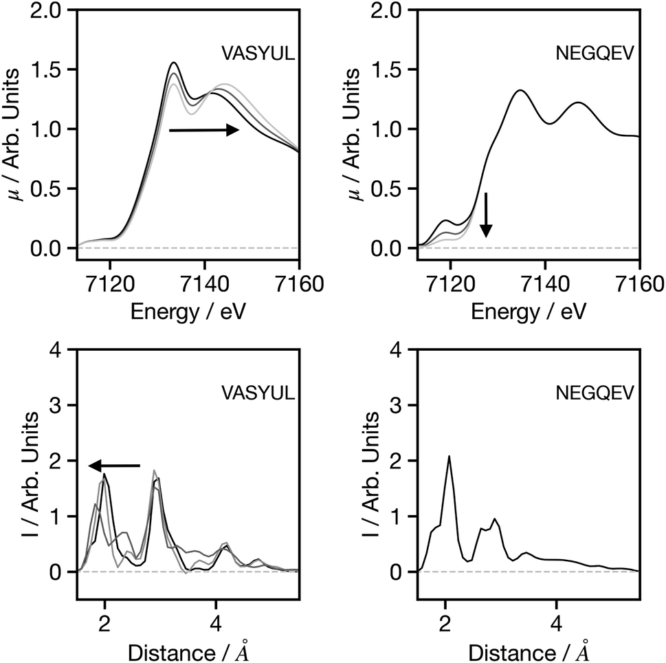 | ||
| Fig. 7 Spectra (upper) and G2 wACSF (lower) where either the energy gap between the two above-ionisation resonances is increased (left) or the pre-edge intensity is decreased (right). The six-letter codes are the Cambridge Structural Database identifiers upon which the original spectra are based. | ||
3.2 Estimating uncertainty of the structural predictions
Having established the performance of the network in terms of predicting the G2 wACSF, we now seek to assess uncertainty using the bootstrap resampling approach outlined in ref. 32. Fig. 8a shows a histogram of the coverage, defined as the percentage of target data points which fall within ±2σ of the average prediction computed using the bootstrap resampling approach for the held-out set. This demonstrates a distribution largely between 45–100%, with a median coverage of 64%, which is smaller than observed for the forward structure to spectrum network,32 but comparable to that reported for X-ray emission spectroscopy.14 While the coverage demonstrates the performance of the uncertainty quantification methods, it can only be used as a metric if the known structure and therefore target G2 wACSF exists, which would negate the purpose for the use of DNN for future applications. Consequently, Fig. 8b shows parity plots of the standard deviation and mean-squared error (MSE) between the calculated and predicted G2 wACSF. The Pearson correlation (ρ) is 0.72, indicating a strong correlation between the MSE and σ, meaning the latter can be effectively used as a metric to assess the accuracy of the prediction. Interestingly, the points that deviate from the main trend shown in Fig. 8b, appear at larger MSE. This suggests, in contrast to recent work32,36 that when the model uncertainty fails, it is slightly over-confident, i.e. the MSE is larger than suggested from that specific σ, which is discussed in the next section.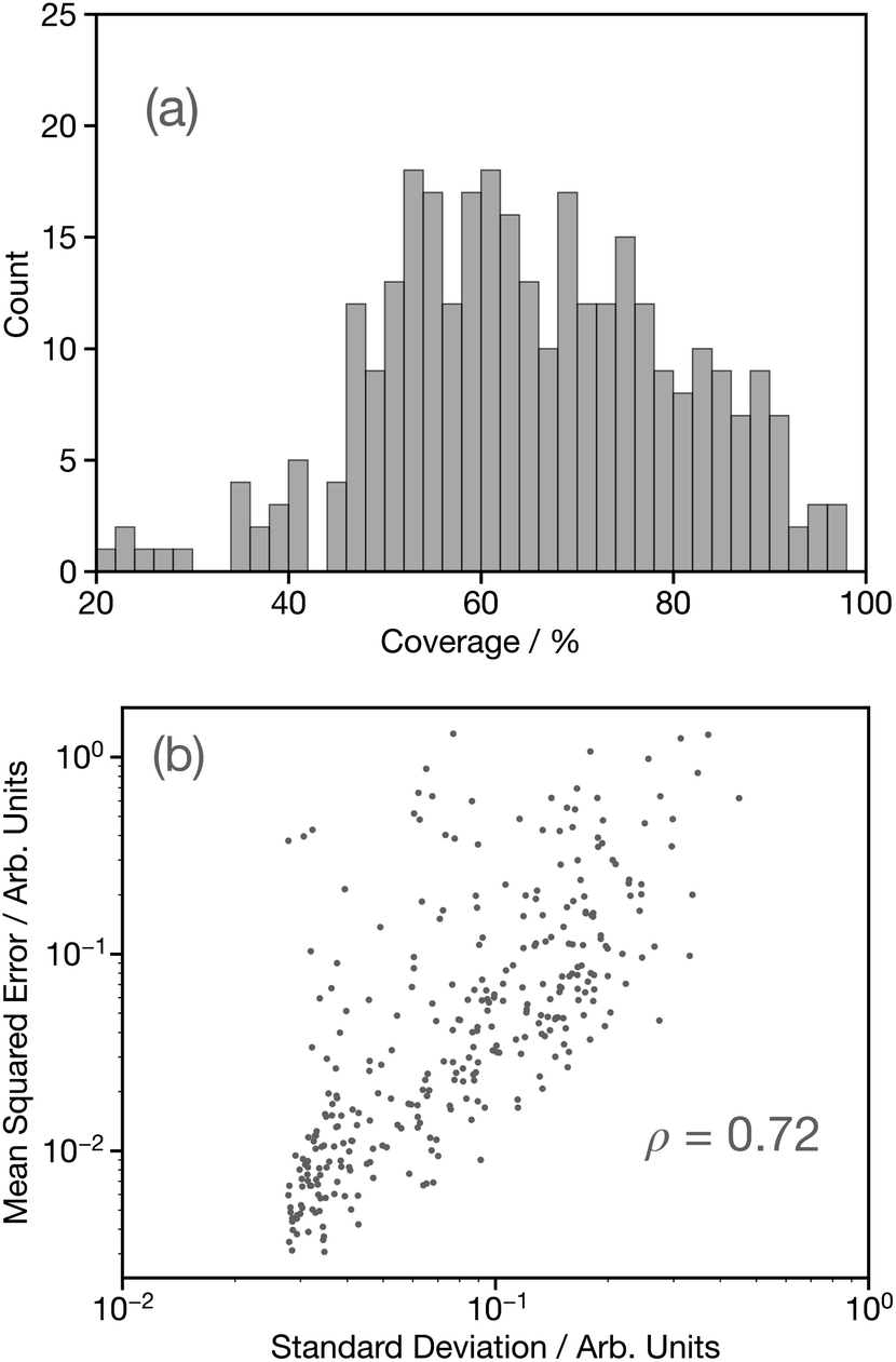 | ||
| Fig. 8 (a) Histograms of the coverage, defined the percentage of target data points which fall within ±2σ of the average prediction computed using the bootstrap resampling approach for the held-out set. (b) Parity plot of the predicted uncertainty against the mean-squared error (MSE) between the predicted, Gpredicted2, and Gtarget2, wACSF calculated using the bootstrap resampling approach. Inset is the value of the Pearson correlation (ρ). | ||
Fig. S4† shows illustrative examples of the G2 wACSF taken from around the median (45th–55th percentile), lower (0th–10th percentile) and upper (90th–100th percentile) when performance is ranked over all held-out DNN predictions by MSE. The light grey traces indicate ±2σ on the predicted G2 wACSF obtained using the bootstrap resampling approach. From Fig. S4,† we observe that as the predictions become worse, the standard deviations become visibly larger, consistent with the parity plot shown in Fig. 8b. For most of the examples shown in Fig. S4,† the 2σ largely follows the MSE, i.e. is large in regions where the MSE is greater. However, the aforementioned slight over-confidence identified is highlighted in DAGPUX, between 3–5 Å, where the error is significant, but the σ is small. The origin of this over-confidence is associated with the Fe–S in the first coordination shell and in discussed in more detail in the following section.
3.3 Applying the network to the analysis of experimental data
As mentioned in the introduction, previous networks that convert spectra into structural information have primarily been utilised with theoretical data. Although valuable for establishing a proof-of-concept, the practical utility of such networks is limited since their focus should be to convert experimental data. To align with our stated objective of achieving a network for XANES which can be equivalent to FT-EXAFS, we are now seeking to apply the network, which was originally developed using theoretical data, to experimental data sourced from ref. 31 and 37–51.Fig. 9 shows 6 G2 wACSF predicted from the experimental spectra of Fe(acac)3,41 [Fe(bpy)3]2+,42 MbO2,38 [Fe(CN)6]4−,48 FeCO5 (ref. 44) and Fe(dedtc)3.49 The first three are within the top 10 of predictions when ranked by MSE, while the latter three are in the bottom 10 predictions. The MSE corresponds to the difference between the predicted and expected wACSF. We note that the expected wACSF for the experimental spectra could be challenging as it does not directly come from the experiment. In the present work the experimental spectra used have been carefully chosen for systems which have well characterised single component systems with structures reported as shown in Table S1.† These single static structures, reported in the publications from where the spectra have been obtained, are either from crystallography or fitting the XANES spectra. While this could potentially be a source of error, it is expected to be small, given the well characterised nature of the spectra and systems chosen. The predictions associated with the remaining 16 experimental spectra are shown in Fig. S4–S6.†
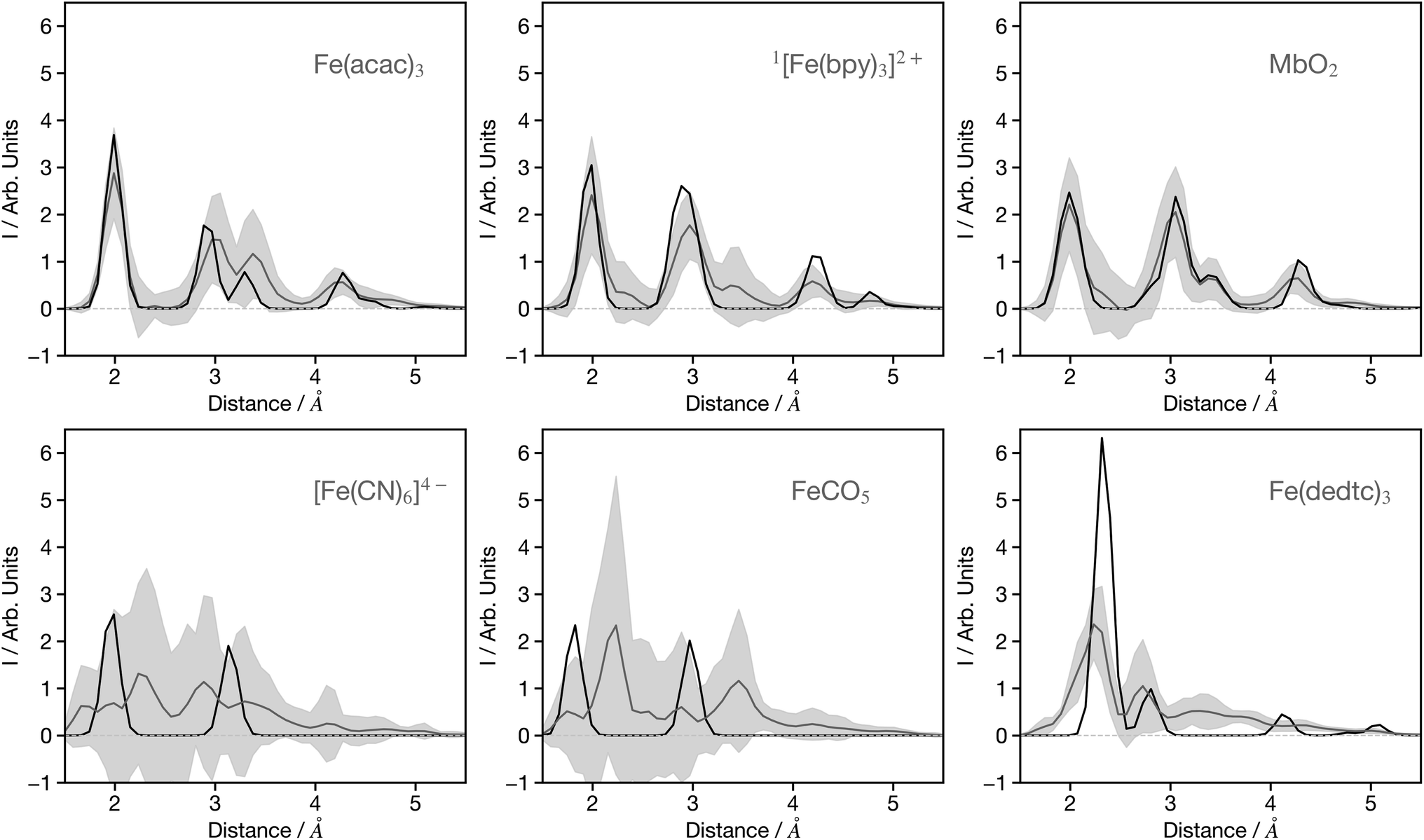 | ||
| Fig. 9 Example G2 wACSF predicted from experimental spectra. The source of the experimental spectra is given in Table S1.† The grey lines are the predicted structures with light grey regions showing ±2σ calculated from the bootstrap resampling. The black traces show the expected G2 wACSF from experimentally reported structures. The upper two panels show three of the top 10 predictions, while the bottom three panels show examples from the worst performers. The remaining examples of transformed experimental spectra are shown in the ESI.† | ||
Fe(acac)3 predicts 4 peaks corresponding to the Fe–O and three Fe–C distances on the acetonylacetonate ligands. The Fe–O distance is 2.0 Å in excellent agreement with expected structure (black line). The predictions for [Fe(bpy)3]2+, in its low spin ground state, captures the first two bands corresponding to the Fe–N and first shell on Fe–C distances. Fig. S4† shows the structural prediction associated with the high-spin state of [Fe(bpy)3]2+. The uncertainty in this prediction, as indicated by the grey shaded area is larger, but remains sufficient to capture the 0.2 Å elongation of the Fe–N bond upon switching from the low to high-spin state.42 MbO2 shows good agreement between the expected and predicted spectrum and is consistent with similar observation made for MbNO and MbCO shown in the Fig. S5.† In contrast, the predictions for related compounds deoxyMb and cytochrome C (Fig. S5†) show worse agreement and a larger uncertainty. This is associated with the underlying theoretical spectra of similar systems in the training sets. In contrast to MbNO, MbCO and MbO2, deoxyMb is a pentacoordinated iron complex, and cytochrome-C has a large Fe–S (2.60 Å) bond meaning that for these latter two systems, the approximated interstitial region in the muffin-tin potentials is large. Therefore, the theoretical spectra will not, for systems like this, provide good agreement with the experiment. The error in these predictions therefore reflect limitations with the underlying training sets.
Three spectra that exhibit poor predictions are shown in the lower 3 panels of Fig. 9. [Fe(CN)6]4− and FeCO5, like other carbonyl and cyanide ligands systems shown in Fig. S4–S6,† show a significant difference between the predicted and expected G2 wACSF, but more importantly a substantial uncertainty. In XANES spectra the scattering pathways along these linear bonds play a larger role than for similar structures containing non-linear bonds due to the focusing effect.52 Recently work addressing the forward mapping (i.e. structure to spectra), highlighted limitations of wACSF descriptor for capturing the focusing effect giving rise to large uncertainties in the associated predictions,32 and our present results clearly exhibit similar limitations for the reverse spectrum to spectra mapping. Fe(dedtc)3 also gives a poor prediction but in contrast to the previous examples a low uncertainty, with the model exhibiting a distinct over-confidence. This is because the structure, consisting of three N,N′-diethyldithiocarbamate ligands, forms a octahedral coordination shell with 6 Fe–S bonds. Such coordination environments are commonly observed in the training set, however, the Fe–S bond length of 2.3 Å leads to a large approximated interstitial region in the muffin-tin potentials, resulting in theoretical spectra that do not agree well with experimental data for such systems. Consequently, although the network is trained on molecules exhibiting a similar structure giving the network a high confidence in the G2 wACSF predictions, it is misplaced because the training data does not accurately represent the experimental observations for such cases.
4 Discussion and conclusions
In this paper we have developed and deployed a CNN which directly transforms XANES spectra into a pseudo radial distribution function, based upon the G2 terms within the wACSF descriptor.28 The core objective of this work is to achieve a simple methodology that directly quantifies structural information in XANES spectra analogous to a FT of an EXAFS spectrum. Our network, trained upon calculated XANES spectra, provides not only accurate translation of simulated data, but importantly demonstrates encouraging insight when applied directly to experimental data. In addition, by combining the network with a bootstrap resampling methodology, our approach can also quantify the uncertainty expected, i.e. how much trust end-users should place in the predictions made by the network.This work sets the foundation for developing reliable models that can routinely translate experimental XANES spectra to provide structural insight. Within the present framework based solely on theoretical data, limitations of the model will arise where theory does not offer a good agreement with its experimental counterpart in term of peak positions and intensities. The training sets in the present work were developed using multiple scattering theory within the muffin-tin approximation. While computationally inexpensive, this approach provided accurate spectra for a large region of the spectrum, especially higher in energy above the absorption edge.30 This is demonstrated by our model reproducing expected physical trends, such as Natoli's rule9 which rely on the above-ionisation resonances.
Although the muffin-tin approximation is a good approximation for large regions of the spectrum, close to the edge, the excited electron is often sensitive to the fine details of the atomic potential leading to a breakdown of the muffin-tin approximation. Such problems are most commonly encountered in the case of open structured systems (i.e. long bond lengths to absorbing atom)53 or when the absorbing atom is not fully coordinated. This means, in both cases, that the approximated interstitial region is large. Our model demonstrates this limitation when it does not reflect structural changes when there are changes in the pre-edge region of the spectrum. It can also be observed in our present analysis of experimental spectra with poor performance for complexes such as Fe(dedtc)3. The obvious solution for this is to use higher levels of theory, which go beyond the MT potential. However care must taken to incorporate the many body effects associated with the high energy photoelectrons which are often important in the XANES intensities.54
Two additional elements when assessing differences between experiment and theory which may affect the performance of the network are the absolute energies and spectral broadening. In this work we have demonstrated that both will have a rather limited influence on the structure predicted, unless the prediction is poor and consequently, these tests, alongside the bootstrap resampling could serve as a metric for assessing confidence.
In summary, this work provides an exciting foundation to deliver quantitative analysis of XANES spectra, equivalent to the FT analysis of EXAFS. The previous discussions highlight that improvements for the current network should focus upon the training data and its use. The most obvious approach would be to train future networks using experimental data, however despite the increasing capacity to record XANES spectra based upon developments such as laboratory based X-ray spectroscopy,55–57 it remains a tall order to record the >1000 spectra required to train a network. One future approach is to incorporate experimental data into the training process, through either mixed training sets or by a transfer learning approach.
Data availability
Data supporting this publication is openly available. The software can be obtained from ref. 27, while the data can be obtained from ref. 29.Conflicts of interest
The authors have no conflicts of interest to declare.Acknowledgements
This research made use of the Rocket High Performance Computing service at Newcastle University. T. J. P would like to thank the EPSRC for an Open Fellowship (EP/W008009/1) and research grant number EP/X035514/1. The authors acknowledge the Leverhulme Trust (Project RPG-2020-268).Notes and references
- F. Lin, Y. Liu, X. Yu, L. Cheng, A. Singer, O. G. Shpyrko, H. L. Xin, N. Tamura, C. Tian and T.-C. Weng, et al. , Chem. Rev., 2017, 117, 13123–13186 CrossRef CAS PubMed.
- T. Katayama, T. Northey, W. Gawelda, C. J. Milne, G. Vankó, F. A. Lima, R. Bohinc, Z. Németh, S. Nozawa and T. Sato, et al. , Nat. Commun., 2019, 10, 3606 CrossRef PubMed.
- D. E. Sayers, E. A. Stern and F. W. Lytle, Phys. Rev. Lett., 1971, 27, 1204 CrossRef CAS.
- T. Penfold, I. Tavernelli, C. Milne, M. Reinhard, A. E. Nahhas, R. Abela, U. Rothlisberger and M. Chergui, J. Chem. Phys., 2013, 138, 014104 CrossRef CAS PubMed.
- J. J. Rehr and R. C. Albers, Rev. Mod. Phys., 2000, 72, 621 CrossRef CAS.
- I. Arcon, B. Mirtic and A. Kodre, J. Am. Ceram. Soc., 1998, 81, 222–224 CrossRef CAS.
- F. Farges, G. E. Brown and J. Rehr, et al. , Phys. Rev. B: Condens. Matter Mater. Phys., 1997, 56, 1809 CrossRef CAS.
- F. De Groot, G. Vankó and P. Glatzel, J. Phys.: Condens. Matter, 2009, 21, 104207 CrossRef PubMed.
- C. Natoli, EXAFS and Near Edge Structure: Proceedings of the International Conference Frascati, Italy, September 13–17, 1982, 1983, pp. 43–56 Search PubMed.
- C. D. Rankine and T. J. Penfold, J. Phys. Chem. A, 2021, 125, 4276–4293 CrossRef CAS PubMed.
- C. D. Rankine, M. M. Madkhali and T. J. Penfold, J. Phys. Chem. A, 2020, 124, 4263–4270 CrossRef CAS PubMed.
- M. R. Carbone, M. Topsakal, D. Lu and S. Yoo, Phys. Rev. Lett., 2020, 124, 156401 CrossRef CAS PubMed.
- C. Rankine and T. Penfold, J. Chem. Phys., 2022, 156, 164102 CrossRef CAS PubMed.
- T. Penfold and C. Rankine, Mol. Phys., 2022, e2123406 Search PubMed.
- J. Timoshenko and A. I. Frenkel, ACS Catal., 2019, 9, 10192–10211 CrossRef CAS.
- J. Timoshenko, A. Halder, B. Yang, S. Seifert, M. J. Pellin, S. Vajda and A. I. Frenkel, J. Phys. Chem. C, 2018, 122, 21686–21693 CrossRef CAS.
- J. Timoshenko, M. Ahmadi and B. Roldan Cuenya, J. Phys. Chem. C, 2019, 123, 20594–20604 CrossRef CAS.
- Y. Liu, N. Marcella, J. Timoshenko, A. Halder, B. Yang, L. Kolipaka, M. J. Pellin, S. Seifert, S. Vajda and P. Liu, et al. , J. Chem. Phys., 2019, 151, 164201 CrossRef PubMed.
- M. R. Carbone, S. Yoo, M. Topsakal and D. Lu, Phys. Rev. Mater., 2019, 3, 033604 CrossRef CAS.
- S. B. Torrisi, M. R. Carbone, B. A. Rohr, J. H. Montoya, Y. Ha, J. Yano, S. K. Suram and L. Hung, npj Comput. Mater., 2020, 6, 109 CrossRef.
- S. Kiyohara and T. Mizoguchi, J. Phys. Soc. Jpn., 2020, 89, 103001 CrossRef.
- M. Higashi and H. Ikeno, Mater. Trans., 2023 DOI:10.2320/matertrans.MT-MG2022028.
- D. P. Kingma and J. L. Ba, arXiv, 2014, preprint, arXiv:1412.6980, DOI:10.48550/arXiv.1412.6980.
- X. Glorot and Y. Bengio, Proceedings of the thirteenth international conference on artificial intelligence and statistics, 2010, pp. 249–256 Search PubMed.
- N. Ketkar, J. Moolayil, N. Ketkar and J. Moolayil, Deep Learning with Python: Learn Best Practices of Deep Learning Models with PyTorch, 2021, pp. 27–91 Search PubMed.
- A. Hjorth Larsen, J. Jorgen Mortensen, J. Blomqvist, I. E. Castelli, R. Christensen, M. Dułak, J. Friis, M. N. Groves, B. Hammer and C. Hargus, et al. , J. Phys.: Condens.Matter, 2017, 29, 273002 CrossRef PubMed.
- XANESNET, 2023, https://gitlab.com/team-xnet/xanesnet Search PubMed.
- M. Gastegger, L. Schwiedrzik, M. Bittermann, F. Berzsenyi and P. Marquetand, J. Chem. Phys., 2018, 148, 241709 CrossRef CAS PubMed.
- XANESNET Training Data, 2023, https://gitlab.com/team-xnet/training-sets Search PubMed.
- J. J. Rehr, J. J. Kas, F. D. Vila, M. P. Prange and K. Jorissen, Phys. Chem. Chem. Phys., 2010, 12, 5503–5513 RSC.
- T. J. Penfold, M. Reinhard, M. H. Rittmann-Frank, I. Tavernelli, U. Rothlisberger, C. J. Milne, P. Glatzel and M. Chergui, J. Phys. Chem. A, 2014, 118, 9411–9418 CrossRef CAS PubMed.
- S. Verma, N. K. N. Aznan, K. Garside and T. J. Penfold, Chem. Commun., 2023, 59, 7100–7103 RSC.
- A. A. Peterson, R. Christensen and A. Khorshidi, Phys. Chem. Chem. Phys., 2017, 19, 10978–10985 RSC.
- M. Annegarn, J. M. Kahk and J. Lischner, J. Chem. Theory Comput., 2022, 18, 7620–7629 CrossRef CAS PubMed.
- T. E. Westre, P. Kennepohl, J. G. DeWitt, B. Hedman, K. O. Hodgson and E. I. Solomon, J. Am. Chem. Soc., 1997, 119, 6297–6314 CrossRef CAS.
- A. Ghose, M. Segal, F. Meng, Z. Liang, M. S. Hybertsen, X. Qu, E. Stavitski, S. Yoo, D. Lu and M. R. Carbone, Phys. Rev. Res., 2023, 5, 013180 CrossRef CAS.
- C. Bacellar, D. Kinschel, G. F. Mancini, R. A. Ingle, J. Rouxel, O. Cannelli, C. Cirelli, G. Knopp, J. Szlachetko and F. A. Lima, et al. , Proc. Natl. Acad. Sci. U. S. A., 2020, 117, 21914–21920 CrossRef CAS PubMed.
- F. A. Lima, T. J. Penfold, R. M. Van Der Veen, M. Reinhard, R. Abela, I. Tavernelli, U. Rothlisberger, M. Benfatto, C. J. Milne and M. Chergui, Phys. Chem. Chem. Phys., 2014, 16, 1617–1631 RSC.
- J. Oudsen, B. Venderbosch, D. Martin, T. Korstanje, J. Reek and M. Tromp, Phys. Chem. Chem. Phys., 2019, 21, 14638–14645 RSC.
- P. D'Angelo and M. Benfatto, J. Phys. Chem. A, 2004, 108, 4505–4514 CrossRef.
- A. Deb and E. J. Cairns, Fluid Phase Equilib., 2006, 241, 4–19 CrossRef CAS.
- C. Bressler, C. Milne, V.-T. Pham, A. ElNahhas, R. M. van der Veen, W. Gawelda, S. Johnson, P. Beaud, D. Grolimund and M. Kaiser, et al. , Science, 2009, 323, 489–492 CrossRef CAS PubMed.
- M. Guo, O. Prakash, H. Fan, L. H. de Groot, V. F. Hlynsson, S. Kaufhold, O. Gordivska, N. Velásquez, P. Chabera and P. Glatzel, et al. , Phys. Chem. Chem. Phys., 2020, 22, 9067–9073 RSC.
- W.-T. Chen, C.-W. Hsu, J.-F. Lee, C.-W. Pao and I.-J. Hsu, ACS Omega, 2020, 5, 4991–5000 CrossRef CAS PubMed.
- A. J. Atkins, C. R. Jacob and M. Bauer, Chem. –Eur. J., 2012, 18, 7021–7025 CrossRef CAS PubMed.
- A. Britz, W. Gawelda, T. A. Assefa, L. L. Jamula, J. T. Yarranton, A. Galler, D. Khakhulin, M. Diez, M. Harder and G. Doumy, et al. , Inorg. Chem., 2019, 58, 9341–9350 CrossRef CAS PubMed.
- V. Briois, C. C. dit Moulin, P. Sainctavit, C. Brouder and A.-M. Flank, J. Am. Chem. Soc., 1995, 117, 1019–1026 CrossRef CAS.
- A. J. Atkins, M. Bauer and C. R. Jacob, Phys. Chem. Chem. Phys., 2015, 17, 13937–13948 RSC.
- S. Mebs, B. Braun, R. Kositzki, C. Limberg and M. Haumann, Inorg. Chem., 2015, 54, 11606–11624 CrossRef CAS PubMed.
- V. Briois, P. Sainctavit, G. J. Long and F. Grandjean, Inorg. Chem., 2001, 40, 912–918 CrossRef CAS.
- C. Mathonière, D. Mitcov, E. Koumousi, D. Amorin-Rosario, P. Dechambenoit, S. F. Jafri, P. Sainctavit, C. C. dit Moulin, L. Toupet and E. Trzop, et al. , Chem. Commun., 2022, 58, 12098–12101 RSC.
- S. Zabinsky, J. Rehr, A. Ankudinov, R. Albers and M. Eller, Phys. Rev. B: Condens. Matter Mater. Phys., 1995, 52, 2995 CrossRef CAS PubMed.
- J. Danese and J. Connolly, J. Chem. Phys., 1974, 61, 3063–3070 CrossRef CAS.
- J. Kas, J. Rehr and J. Curtis, Phys. Rev. B, 2016, 94, 035156 CrossRef.
- P. Zimmermann, S. Peredkov, P. M. Abdala, S. DeBeer, M. Tromp, C. Müller and J. A. van Bokhoven, Coord. Chem. Rev., 2020, 423, 213466 CrossRef CAS.
- Z. Németh, J. Szlachetko, É. G. Bajnóczi and G. Vankó, Rev. Sci. Instrum., 2016, 87, 103105 CrossRef PubMed.
- G. Seidler, D. Mortensen, A. Remesnik, J. Pacold, N. Ball, N. Barry, M. Styczinski and O. Hoidn, Rev. Sci. Instrum., 2014, 85, 113906 CrossRef CAS PubMed.
Footnote |
| † Electronic supplementary information (ESI) available. See DOI: https://doi.org/10.1039/d3dd00101f |
| This journal is © The Royal Society of Chemistry 2023 |