
 Open Access Article
 This Open Access Article is licensed under a Creative Commons Attribution-Non Commercial 3.0 Unported Licence
A rheologist's guideline to data-driven recovery of complex fluids' parameters from constitutive models
Milad
Saadat
 ,
Deepak
Mangal
and
Safa
Jamali
*
,
Deepak
Mangal
and
Safa
Jamali
*
Department of Mechanical and Industrial Engineering, Northeastern University, Boston, 02115 Massachusetts, USA. E-mail: s.jamali@northeastern.edu
First published on 26th June 2023
Abstract
Rheology-informed neural networks (RhINNs) have recently been popularized as data-driven platforms for solving rheologically relevant differential equations. While RhINNs can be employed to solve different constitutive equations of interest in a forward or inverse manner, their ability to do so strictly depends on the type of data and the choice of models embedded within their structure. Here, the applicability of RhINNs in general, and the interplay between the choice of models, parameters of the neural network itself, and the type of data at hand are studied. To do so, a RhINN is informed by a series of thixotropic elasto-visco-plastic (TEVP) constitutive models, and its ability to accurately recover model parameters from stress growth and oscillatory shear flow protocols is investigated. We observed that by simplifying the constitutive model, RhINN convergence is improved in terms of parameter recovery accuracy and computation speed while over-simplifying the model is detrimental to accuracy. Moreover, several hyperparameters, e.g., the learning rate, activation function, initial conditions for the fitting parameters, and error heuristics, should be at the top of the checklist when aiming to improve parameter recovery using RhINNs. Finally, the given data form plays a pivotal role, and no convergence is observed when one set of experiments is used as the given data for either of the flow protocols. The range of parameters is also a limiting factor when employing RhINNs for parameter recovery, and ad hoc modifications to the constitutive model can be trivial remedies to guarantee convergence when recovering fitting parameters with large values.
1 Introduction
The nature of time- and rate-dependent responses of complex fluids to an applied deformation makes their modeling both extremely important and challenging simultaneously: one would need to predict the material response accurately, which is generally proven far from trivial. In complex fluid modeling, a critical component is the choice of the constitutive model that relates the components of the deformation [tensor] to the shear stress [tensor]. Whether bottom-up modeling, for example, in polymer melts1 or phenomenological modeling using simple but meaningful assumptions about material responses,2–4 rheology actively witnesses new constitutive models (CMs) for different fluid flows and characteristics. Depending on the material [and the condition] one wishes to shed light upon, these may include simple Generalized Newtonian Fluid models that account for a rate-dependent viscosity5,6 or systems of differential equations in which the time-dependent response of the fluid is accounted for as well.7–10Under shear flows,† material responses roughly fall into viscous, elastic, plastic, and thixotropic categories, the barriers of which are often so blurred that even experts may dispute the true nature of certain flow observations. Nonetheless, one could argue that the most complex rheological behavior is observed in so-called “thixotropic elasto-visco-plastic (TEVP)” materials, where all the different material characteristics mentioned above can be observed over time. As noted in Larson's reviews,11,12 thixotropy is far from a mere continuous decrease of viscosity with time (which is also seen for viscoelastic materials) and has to do with the material's memory of the entire flow history.13,14 Generally, one popular and effective way of modeling thixotropic behavior is through the introduction of a quantitative measure to the material's microstructure. The extent of microstructure breakdown or formation can be approximated through a competition between shearing forces that break down the structure and the natural structuration of the material.15–17 Ultimately, the resulting constitutive relations that are commonly used to model complex fluids can be coupled differential equations. These coupled ordinary differential equations (ODEs) get more complex as the behavior in question gets more intricate.
The concept of digital discovery in complex fluid modeling can be viewed from two angles: (i) a particular constitutive model is known to be the appropriate choice, and one may be interested in the discovery of the solution, given the model parameters and boundary and/or initial conditions (forward problem), or (ii) a particular measurement with respect to input variables is made, and the objective is to discover the appropriate model and/or its parameters (inverse problem) that best describe the material's behavior. For the former, decades of research have been invested in developing algorithms and commercial packages that solve the equations of interest analytically or numerically.18–21 These algorithms, however, often struggle in the face of inverse problems and ill-posedness,22 meaning that a solution may be either nonexistent or not unique. One may tackle ill-posed or inverse problems by performing a parametric sweep on the unknown parameters; the recovery, however, becomes prohibitive as the number of unknown parameters to be recovered increases, which is common in rheological constitutive models. Data-driven methodologies, on the other hand, have proven to be transformative in the sense that they can tolerate ill-posedness and are suitable choices when tackling inverse [and forward] problems23 to provide unified platforms for the discovery of complex fluids and flows.
Over the past few years, several efforts have been made to leverage the advent of artificial intelligence (AI) and machine learning (ML) to obtain forward and inverse solutions of differential equations alike.24–29 In particular, physics-informed neural networks (PINNs) were revived by incorporating model equations into the neural network (NN) framework for forward and inverse analysis and surrogate modeling of many scientific problems.30,31 In rheology, a few rheology-informed neural network (RhINN) platforms were developed by informing the neural network of the underlying rheological CMs, both implicitly and explicitly.32–36 Other efficient and promising data-driven algorithms and tools have also been developed to recover parameters in rheological problems of interest.37–41 Owing to their robust automatic differentiation capabilities27 and excellent generalizability, RhINNs can act as a unifying framework for the digital discovery of complex fluids. Moreover, due to the flexibility in tweaking the NN parameters, the ill-posedness issue can be dramatically mitigated in RhINNs. This work focuses explicitly on inverse problems and parameter recovery using RhINNs.
When employing RhINNs, or other predictive methods deemed to recover the fitting parameters of a CM, one may consider three elements in close relationship with each other, i.e., the CM whose fitting parameters are asked for, the predictive method (the neural network in the case of RhINNs), and the data at hand. In rheologically relevant problems of interest, the latter is usually composed of the imposed actuation (e.g., shear rate), time of the experiment, and the measured quantity (e.g., shear stress or viscosity). Most frequently, the data are given, and the fitting parameters of a particular CM are requested by interrogating the predictive method. It is thus necessary to study the effect of the predictive method's hyperparameters, which are selected [and optimized] before the training process. However, it is generally not reported as to what extent the predictions are influenced by the interplay between hyperparameters, the CM, and the data, despite solid evidence that such an interplay may impact [or limit] the number of parameters one is able to recover and their range.37
For instance, our recent work used experimental data (i.e., steady-state viscosity vs. shear rate) spanning over six decades in magnitude and embedded several steady-state constitutive models in a RhINN platform.‡ It was shown that RhINNs can select the best [yet simplest] constitutive model representing each experimental behavior and also recover the parameters of all constitutive models. Also, the effect of a systematic reduction in the data size and range was studied.36 In other words, among the three intercoupled components mentioned above, the interplay between constitutive models and data was explored, but the neural net hyperparameters were fixed [and assumed optimized], which is also the trend in the literature. As the next natural step, we intend to explore the interplay between the choice of constitutive models whose parameters will be recovered using RhINNs, the neural network itself, and the transient data at hand. In particular, we seek to answer the following question: How much can we push a RhINN platform (the CM, the neural net, and the data) before it loses its predictive capabilities? This question was partially answered for fixed RhINN hyperparameters and a thixotropic elasto-visco-plastic (TEVP) model using only flow startup data during the training step.32 Here, to answer this question more comprehensively, we relaxed the assumptions mentioned above. To this end, a set of flow startup data is generated, and the RhINN is requested to recover the fitting parameters of several simple-to-complex TEVP cases. Also, the hyperparameters in an inverse problem are varied, and those with the highest impact on parameter recovery are reported. Moreover, the data, in terms of their size and range for shear startup and oscillatory flow protocols, are carefully examined to gauge the sensitivity of parameter recovery as a function of the flow protocol. We deliberately attained a tutorial tone in this work since a comprehensive study circumscribing the applicability of RhINNs, to the best of our knowledge, is yet to be reported. Although tailored for rheology, this walk-through study can provide important information about the inverse solution of [coupled] differential equations using PINN platforms in general, their inherent capabilities [and limitations], and specific scenarios where those do not present the best course of action.
2 Methods
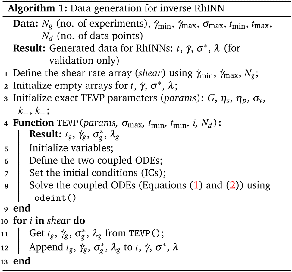
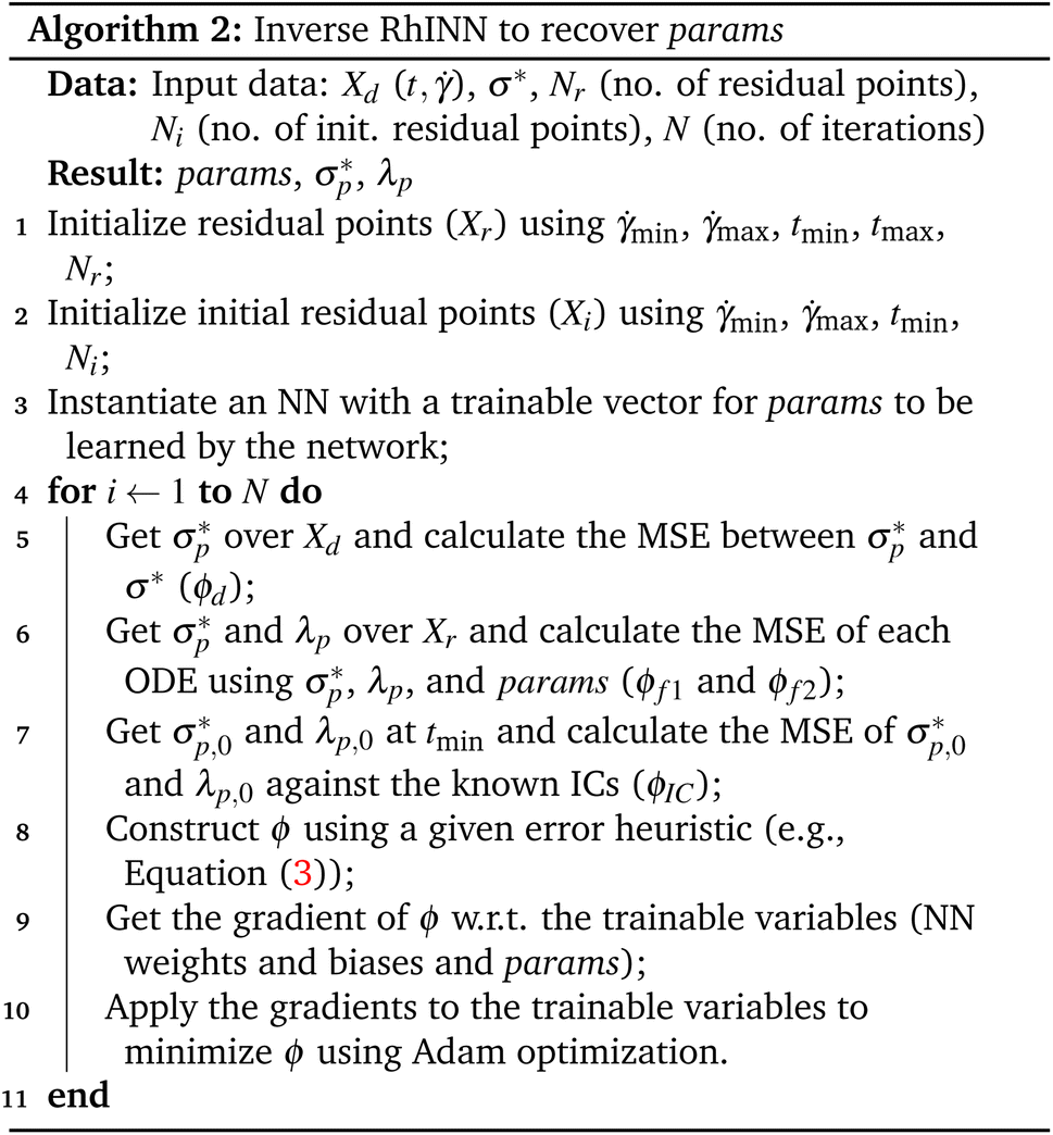
In statistical neural networks (NNs), one merely deals with a set of given data, the NN itself, and NN predictions of target variables. In Fig. 1, such NNs are possible by removing the green box, allowing the NN to adhere to some physical intuition. However, the intent here is to recover the fitting parameters of a constitutive model (CM); thus, a functional form (i.e., the CM here) needs to be embedded into the neural network architecture, similar to other solvers for inverse problems. The approach to do so is discussed in Section 2.1. The predictive method (RhINN) and its hyperparameters will then be discussed in Section 2.2. Next, in Section 2.3, the data in terms of their type, size, and range are introduced. These three components are color-coded in Fig. 1 and are shown in more detail in Fig. 2. The pseudo-codes to generate the ground-truth data and perform the training step are also presented in Algorithms 1 and 2, respectively, to facilitate the implementation using other packages or in other languages.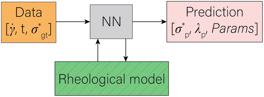 | ||
Fig. 1 The general structure of a rheology-informed neural network (RhINN) with two inputs (![[small gamma, Greek, dot above]](https://www.rsc.org/images/entities/i_char_e0a2.gif) and t) and two outputs ( and t) and two outputs ( and λp). The constitutive model's parameters (Params) are defined as trainable and are a part of the neural net output. The given data are the ground-truth normalized shear stress response and λp). The constitutive model's parameters (Params) are defined as trainable and are a part of the neural net output. The given data are the ground-truth normalized shear stress response  as a function of the imposed shear rate and time t. Note that there are no data to train λp separately, and λp is learned using the coupled ODEs defined in Section 2.1. For the case of oscillatory shear flows (see Section 2.3), is replaced with the strain amplitude, γ0. as a function of the imposed shear rate and time t. Note that there are no data to train λp separately, and λp is learned using the coupled ODEs defined in Section 2.1. For the case of oscillatory shear flows (see Section 2.3), is replaced with the strain amplitude, γ0. | ||
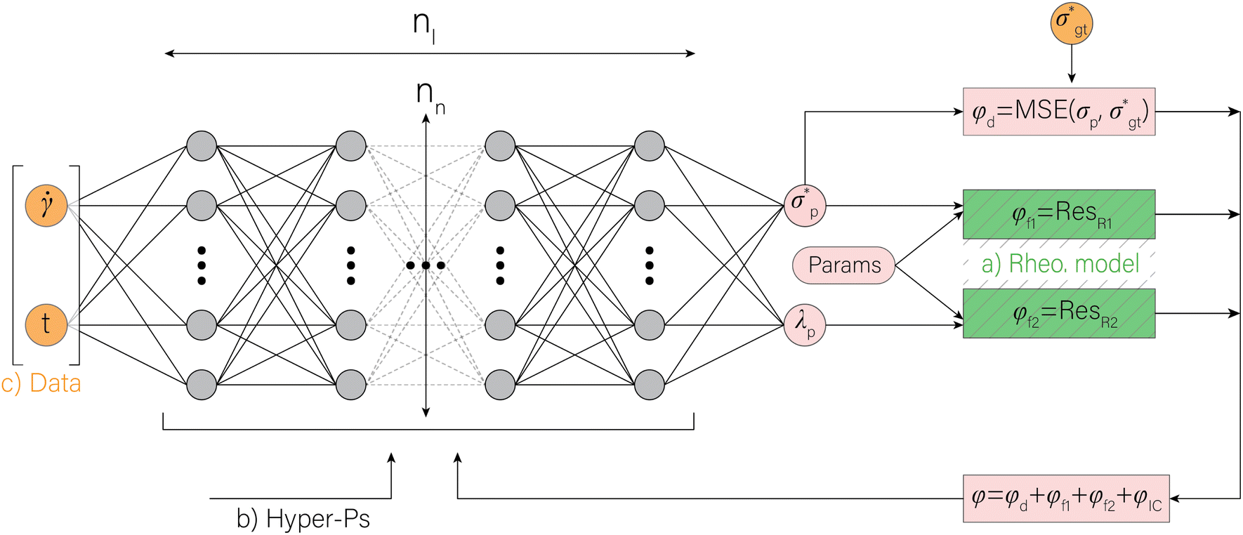 | ||
Fig. 2 A closer look at the rheology-informed neural network (RhINN) with nl layers, each containing nn neurons. In this illustration, the input layer containing two inputs ( and t) is fully connected to the subsequent hidden layers. The outputs ( , λp, and the CM's parameters, Params) are then used to calculate a loss function consisting of a data discrepancy part (ϕd), one residual for each ODE of the TEVP model, and an initial condition loss (ϕIC). Note that Params are not connected to the layers and are updated since they are a part of the ODE losses. In this work, the interplay between the rheological model (a), RhINN's hyperparameters (b), and the data (c) is studied. ϕd only accounts for the normalized shear stress discrepancy since no physical data for the structure parameter (λ) can be obtained from rheometry. The goal is to recover the fitting parameters of the rheological model, i.e., the TEVP model. The components of this figure are color-matched with those of Fig. 1 for easier tracking. For the case of oscillatory shear flows (see Section 2.3), is replaced with the strain amplitude, γ0. , λp, and the CM's parameters, Params) are then used to calculate a loss function consisting of a data discrepancy part (ϕd), one residual for each ODE of the TEVP model, and an initial condition loss (ϕIC). Note that Params are not connected to the layers and are updated since they are a part of the ODE losses. In this work, the interplay between the rheological model (a), RhINN's hyperparameters (b), and the data (c) is studied. ϕd only accounts for the normalized shear stress discrepancy since no physical data for the structure parameter (λ) can be obtained from rheometry. The goal is to recover the fitting parameters of the rheological model, i.e., the TEVP model. The components of this figure are color-matched with those of Fig. 1 for easier tracking. For the case of oscillatory shear flows (see Section 2.3), is replaced with the strain amplitude, γ0. | ||
2.1 Constitutive model
To explore the interplay between the neural net (referred to as NN in this work), the constitutive model (CM), and the data, it is best to start with the CM whose parameters are to be recovered. As a rheologically motivated example, a thixotropic elasto-visco-plastic (TEVP) constitutive model8,32,42,43 is chosen, which consists of two coupled ODEs. In this formalism, eqn (1) describes the time evolution of the normalized shear stress, σ*(t), which is the actual shear stress, σ(t), divided by the maximum shear stress of the sample (σmax):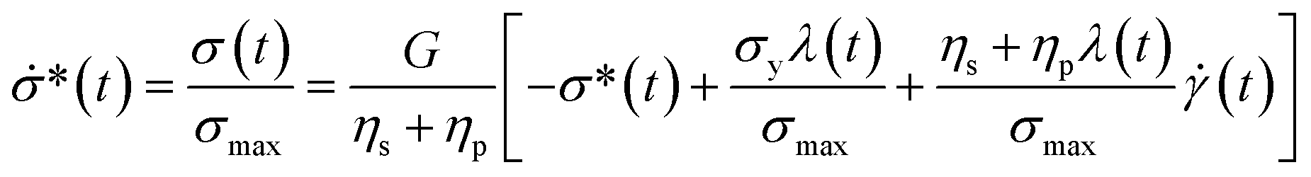 | (1) |
(t), in s−1, is the imposed shear rate (assuming a rate-controlled rheometry), and λ(t) is the dimensionless structure parameter. λ(t) represents the instantaneous extent of the microstructure of the fluid under flow and is the hallmark of thixotropic constitutive models. The variations of λ in time was proposed to obey the following:12,16,32,44| (t) = k+(1 − λ(t)) − k−λ(t)(t) | (2) |
(t)) and formation due to the natural affinity of material components to aggregate/assemble. A λ equal to unity translates to a fully structured material, whereas λ = 0 corresponds to a fully destructured fluid. The time evolution equation for calculating this structure parameter can take more complex forms. For instance, the HAWB model45 introduces a shear-induced aggregation term within this formalism. TEVP fluids can also be modeled through fluidity models in which the fluidity is generally defined as the inverse of this structural measure.46 Note that beyond the time evolution equation for the shear stress and the structure formation/breakdown, additional closed-form equations can be introduced to account for the flow directionality and/or other memory effects, such as the Bauschinger effect. For instance, iso-kinematic hardening (IKH) models7,47 consider an additional equation for measuring a back-stress, which is then used to calculate the dissociated elastic versus plastic deformations.
It is worth mentioning that by normalizing the shear stress, the range of ODE outputs (σ* and λ) will remain the same. Without doing so, shear stress naturally takes a wide range of values depending on the applied deformation rate and material properties, while the structure parameter is constrained between zero and unity, which can cause numerical instabilities commonly encountered in gradient-based optimization tasks. In total, eqn (1) and (2), in their original form, have six fitting parameters, i.e., G, ηs, ηp, σy, k+, and k−.
In Section 3.1, the sensitivity of the neural network's parameter recovery to the complexity of ODEs embedded within its structure will be sought. Thus, the CM (eqn (1) and (2)) is systematically simplified (or inversely complicated) by reducing (or increasing) the number of fitting parameters while keeping the neural net hyperparameters and the data intact. This is far from trivial, as shown in our previous work on the steady-state model selection: the constitutive model's increased complexity may or may not contribute to its predictability, and oversimplified models may fail to capture the delicacies of a material response.36 In other words, the most sophisticated model is not necessarily always the best, and the balance between simplicity and predictability can be obtained through available data-driven approaches.
Throughout this work, eqn (1) and (2) are used to generate the transient data, while the governing CM of choice embedded in RhINNs is systematically altered from a five-parameter model to a ten-parameter one to study the role of model complexity on the predictive capability of RhINNs. These constitutive models are summarized in Table 1.
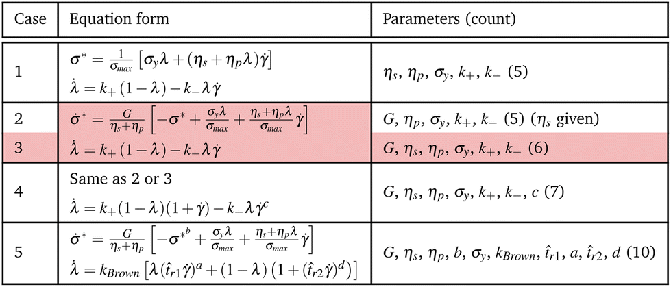
|
2.2 RhINNs
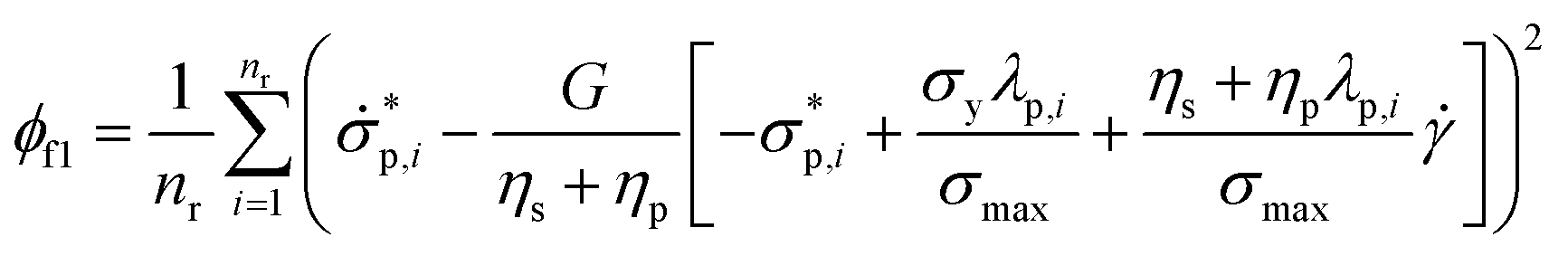
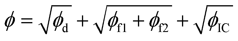
In this section, the concepts relevant to RhINNs [and their subsequent results in Section 3.2] are introduced, assuming that the original TEVP model (Case 3 in Table 1) is embedded. The goal is to provide a reproducible and interoperable platform that can be employed by the community and adaptable to other similar problems. The neural network is built by sub-classing a Keras model49 on TensorFlow v2.10.0. By including a CM (eqn (1) and (2)), a loss function (ϕ) for each iteration is calculated as follows:| ϕ = ϕd + ϕf1 + ϕf2 + ϕIC | (3) |
 and the ground-truth normalized shear stress
  , defined as the following mean-squared error (MSE):
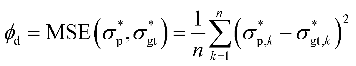 | (4) |
Moreover, the residual (Res in Fig. 2) of the two sides of the normalized shear stress and structure parameter ODEs (ϕf1 and ϕf2, respectively) can be calculated, which is also a mean-squared error:
 | (5) |
and t). Similarly, ϕf2 is calculated as follows: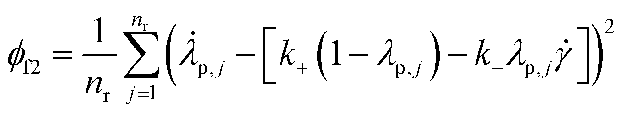 | (6) |
Finally, an initial condition (IC) loss can be calculated, consisting of the MSE of the predicted σ* and λ values at t = 0, i.e., ϕIC. For each output, one IC can be realized. For instance, if σ* and λ at t = 0 are zero and one, respectively, ϕIC is calculated as follows:
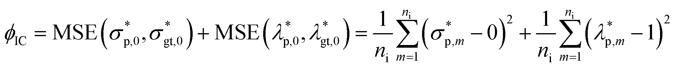 | (7) |
In fully connected NNs, several hidden layers link the inputs to the outputs. Such links are denoted by the connecting lines in Fig. 2. Each layer has a number of neurons, which have trainable weights and biases. In Fig. 2, the number of hidden layers and neurons in each hidden layer is denoted by nl and nn, respectively. In addition, the six fitting parameters that will be recovered (Params in Fig. 2) are trainable, defined as follows in the code:
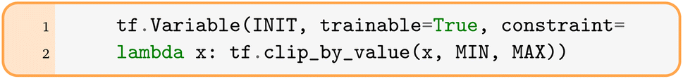
By simply adding eqn (4)–(7) in each iteration, the total loss (eqn (3)) is calculated. Then, by taking the gradient of this total loss with respect to the trainable variables (the weights, biases, and the six fitting parameters) and applying these gradients to the trainable variables, new weights, biases, and fitting parameters are calculated in each iteration to reduce and eventually minimize the total loss, ϕ. It is worth mentioning that tf.GradientTape handles the calculation of gradients in eqn (5) and (6) plus the one mentioned above. Since the total loss includes both the data and the residual losses, the final result after the minimization process will respect both the data and the physical intuition induced during the training process. The loss minimization task is handled by TensorFlow's built-in tf.keras.optimizers.Adam optimizer. The entire optimization task (after the calculation of the loss terms) can also be performed using scipy.optimize.minimize's L-BFGS-B method in the code, but since this method is more computationally expensive than Adam, it is more convenient to perform Adam and use L-BFGS-B if need be. The interested reader is referred to the publicly available codes on the group's GitHub repository§ and also the indexed repository50 for a more detailed explanation.
NN hyperparameters, or in general, hyperparameters in ML, can be thought of as parameters that are external to the model, whose values cannot be estimated from the data. In other words, hyperparameters are tuned before the training process. The following hyperparameters are virtually always studied in every NN implementation:
1. Network depth (the number of hidden layers, nl),
2. Network width (the number of neurons in each layer, nn),
3. Learning rate, lr,
4. Kernel initializer,
5. Activation function, and
6. The seed to generate random numbers.¶
The learning rate and kernel initializer determine the degree of adjustment for the trainable variables and their initial distribution, respectively. The activation (or transfer) function specifies the response of a neuron to the input signal, which is usually a nonlinear function (e.g., tanh) for hidden layers and a linear one for the output layer. The seed assures that the randomization of variables and parameters is consistent from one code run to another.
There are, however, several hyperparameters that are specific to an inverse problem using RhINNs:
7. Initial conditions for the fitting parameters, INIT,
8. Bounds for the fitting parameters, i.e., MIN and MAX, and
9. The error heuristics.
The initial conditions' anticipated effect is similar to other numerical procedures, and convergence may be compromised for unphysical ICs. The parameter bounds may also impact the optimization path during the training process. Most importantly, the error heuristics is expected to directly influence parameter recovery and the overall loss. Other than eqn (3), there are other [ad hoc] ways to calculate ϕ, namely:
1. ϕ = (ϕd + ϕf1 + ϕf2 + ϕIC) × ϕmax
2. 
3. 
where ϕmax is the maximum loss between the three loss components (ϕd, ϕf1 + ϕf2, and ϕIC) at each iteration. Of course, such heuristics are arbitrary, and one can define many more. While there is strong scientific evidence that supports one and discards the others, these few cases are selected to show if tweaking the heuristics should be an option when a researcher has convergence issues for the default case, i.e., eqn (3).
In Section 3.2, these nine hyperparameters are tuned to gauge the sensitivity of the training process and parameter recovery to each of them and hopefully discard a few less-important ones.
2.3 Data analysis
The type of data at hand is low-dimensional; the only inputs are the imposed shear rate and time, and the output is the normalized ground-truth shear stress, . Using eqn (1) and (2) (again, the CM is fixed in this section and Section 3.3), known fitting parameters, and one initial condition for each ODE, a three-dimensional data set (, t, and
  ) is generated using SciPy's odeint method19 and fed to the neural net. Thus, the goal is to recover the fitting parameters whose ground-truth values are available. In this work, the analysis is performed by studying the synthetically generated data (as opposed to seeking digitized experimental measurements from the literature) because by doing so, the ground-truth fitting parameters can be tuned to evaluate to what extent RhINNs can withstand parameters with irregular ranges.
The relationship between , t, and  is determined by the selection of flow protocols, which manifest themselves in the flow curves. Four examples of such flow curves are shown in Fig. 3 using the Maxwell viscoelastic constitutive model, which can be written as:2
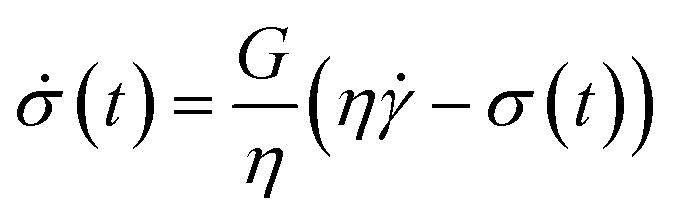 | (8) |
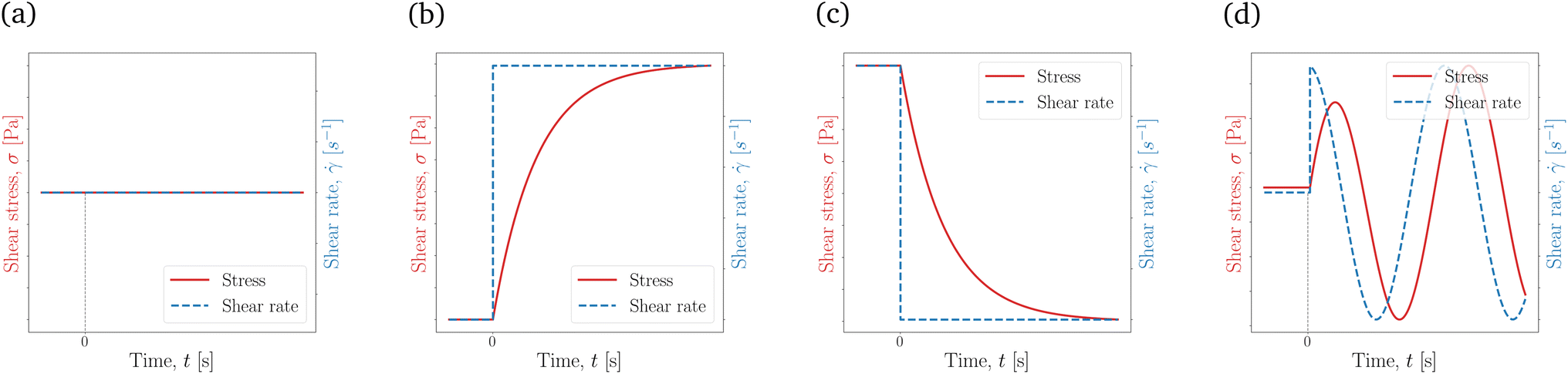 | ||
Fig. 3 Different flow curves generated using a simple Maxwell viscoelastic model, eqn (8). These flow curves, with the increment in complexity, are the (a) steady state shear stress response with = 0, where 0 is constant, (b) stress growth with |t=0+ = 0, (c) stress relaxation with |t=0− = 0, and (d) oscillatory shear with |t=0− = 0 and |t=0+ = γ0ω![[thin space (1/6-em)]](https://www.rsc.org/images/entities/char_2009.gif) cosωt. Generally, as the flow protocol (the input set of data to the NN) gets more complicated, richer physics can be extracted from the data. cosωt. Generally, as the flow protocol (the input set of data to the NN) gets more complicated, richer physics can be extracted from the data. | ||
Typically, flow curves such as the ones in Fig. 3 are obtained directly from a rheometer, where the imposed actuation is the shear rate, , in a rate-controlled experiment or the shear stress, σ, in a stress-controlled experiment. It is worth mentioning here that the focus in this work is on shear rheometry, i.e., a single off-diagonal component of the stress/deformation tensor with respect to the flow and gradient directions. Other viscometric functions, such as normal stress differences and/or extensional viscosity, are directly related to the diagonal components of the stress/deformation tensor and thus require a fully tensorial implementation of the constitutive model as opposed to a scalar description; see the footnote in Section 1.
Starting from the simplest relationship, i.e., when is constant in time ( = 0), the shear stress response is also constant in time, shown in Fig. 3a. With this flow protocol, not much is revealed from the material response except for the shear viscosity, η. Moving on to transient experiments, the material can be subject to a flow startup from quiescent ICs, σ|t=0− = 0, and |t=0+ = 0. This is also referred to as the stress growth test, with the actuation and the σ response shown in Fig. 3b. Cessation of flow at t = 0 from a steady shear, |t=0− = 0 and |t=0+ = 0, also called the stress relaxation test, can be performed instead; see Fig. 3c. Finally, as a more complex test, and starting from quiescent ICs, one may start shearing a material periodically, |t=0− = 0 and = γ0ωcosωt, where γ0 is the oscillation (strain) amplitude and ω is the angular frequency of the imposed shear; see Fig. 3d. Such oscillatory shear flows, depending on the γ0 magnitude, are commonly referred to as small, medium, or large amplitude oscillatory shear (SAOS, MAOS, and LAOS, respectively), which probes into linear and non-linear responses of the fluid.
As mentioned above, a steady-state flow protocol will provide no temporal information, and thus only transient protocols are considered for this work. Among the options mentioned (and other flow protocols commonly used in the rheological literature2), the stress growth and the oscillatory shear protocols [as the simpler and more sophisticated rheological tests] are employed in this work, and their effects on parameter recovery are investigated. For the initial conditions of these two flow types, at t = 0, the material is stress-free and fully structured, meaning that  and λ0 = 1. It is vital to mention that the shear rate () input is replaced with the strain amplitude, γ0 for the case of oscillatory flows in the code, as γ (or ) is a function of both time and the strain amplitude (γ = γ0sinωt). The NN's tf.GradientTape method calculates the partial derivative, and if γ (or ) is used as an input (instead of γ0), then calculating in eqn (5) and (6) requires the application of the chain rule, which is feasible within the framework but adds unnecessary complications in the formulations. It is thus recommended to separate the NN inputs as much as possible to prevent mathematical ambiguities.
Please note that the list of flow protocols, choice of models, and the variations possible within the neural network's architecture can quickly become exhaustive and prohibitive. Thus, here and in the following sections, the effect of given data is studied in terms of:
1. The flow protocol (stress growth or oscillatory shear),
2. The number of tests (i.e., experiments) for each flow protocols,
3. The number of data points in time for each experiment,
4. The observation time window in the oscillatory shear case, and
5. The range of original TEVP parameters for the stress growth test.
3 Results & discussion
3.1 Constitutive model's complexity
To categorically study the results from neural network predictions, the definition of output results (what is being plotted) should be clearly given, as it sometimes significantly deviates from what numerical or experimental studies report. NNs, as a surrogate map, have predictive capabilities by calling the model.predict method. Due to its nonlinear activation functions, RhINN is a nonlinear solver, and as it gets deeper and wider (Section 2.2), the degree of non-linearity increases. However, the embedded CM might be simpler (or more complex), and by inserting the recovered parameters into the CM, the recovered phenomenon may [and will] be different than the NN output. Thus, in inverse problems where the objective is to recover model parameters, it is often misleading to plot the NN predictions using model.predict. Instead, the CM's parameters recovered by the RhINN will be fed into an ODE solver (e.g., SciPy's odeint method19) to solve for the two unknowns, i.e., the normalized shear stress (σ*) and the structure parameter (λ), which makes this step a forward problem. In the following figures, only the RhINN predictions using the recovered parameters are shown, i.e., the red curves; see Fig. 4. | ||
| Fig. 4 RhINN's predictions with an embedded thixotropic visco-plastic (TVP) constitutive model. (a) The normalized shear stress (σ*) and (b) the structure parameter (λ) response for an input shear rate of = 0.5 s−1, which is a shear rate not included in the training data. In this figure, the blue curve represents the neural net's response by calling TensorFlow's model.predict method. However, we are mainly interested in knowing the constitutive model's response using the recovered parameters that the RhINN is returning. To do so, the recovered parameters are fed into their respective ODE form (TVP in this case and TEVP for the rest), and the coupled ODEs are solved using SciPy's odeint method. In all that follows, the plots represent the latter (the red line), meaning that the NN's normalized shear stress (and structure parameter) predictions are discarded as they do not have suitable extrapolation capabilities. The recovered TVP parameters, i.e., σy, ηs, ηp, k+, and k−, are 2.69 Pa, 1 × 10⁻⁴ Pa s, 5.26 Pa s, 1 × 10⁻⁴ s−1, and 1 × 10⁻⁴, respectively. Moreover, the MSE of the predicted σ* (the MSE between the dashed line and the red one) is 5.34 × 10⁻². | ||
To generate data in this section, eqn (1) and (2), the stress growth flow protocol (Fig. 3b) at four shear rates (0.1, 0.4, 0.7 and 1.0 s−1), and fitting parameters listed in Table 2 are used. Then, to test parameter recovery, the σ* and λ responses at = 0.5 s−1 (which was not a part of the given data) are plotted using the recovered parameters. Also, RhINN hyperparameters and the data are all held constant in this section and are summarized in Table 3.
| G [Pa] | σ y [Pa] | η s [Pa s] | η p [Pa s] | k + [s−1] | k − [1] |
|---|---|---|---|---|---|
| 40 | 10 | 10 | 5 | 0.1 | 0.3 |
| Item | Symbol | Value |
|---|---|---|
| NN layer count (depth) | n l | 4 |
| NN neuron count (width) | n n | 20 |
| Learning rate | lr | [1 × 10⁻², 2 × 10⁻³, 1 × 10⁻³] |
| Kernel init. | — | glorot_normal |
| Activation function | — | tanh |
| Initial condition | INIT | 1. for all six parameters |
| Parameter bounds | MIN, MAX | [1 × 10⁻⁴, np.infty] for all six |
| Seed | — | 42 |
| Data on shear rate | — | 0.1, 0.4, 0.7 and 1.0 s−1 |
| Number of points in time | — | 201 |
| Time range | — | [0.01, 100] |
The σ* and λ responses using the thixotropic visco-plastic (TVP) constitutive model embedded in the RhINN (while the given data are still TEVP) are depicted in Fig. 4. For the TVP model, the stress form is no longer an ODE; see Table 1, Case 1. In other words, the TVP model assumes that the elastic response in a material has already faded. However, by embedding the TVP model in the RhINN while using the TEVP model to generate the input data, parameter recovery is unsatisfactory, and the subsequent σ* and λ responses are inaccurate. This is important because one might be tempted to use a constitutive model that is too simple for the given data type. If one strays too far from the given data and resorts to an over-simplified constitutive model, the convergence and accurate parameter recovery seem quixotic, if not impossible. In other words, by removing the elastic component of the constitutive model, the NN loses its entire predictive capability.
Table 4 summarizes the effect of tweaking the CMs on the MSE of σ* and the code execution time in min. The number of parameters to be recovered is also included for easier comparison. As the CM is gradually made more complex from its original form (Case 3), the execution time increases, and the prediction accuracy is reduced. Taking Case 3 as the baseline, this finding indicates that the added parameters do not have explanatory capabilities in general.
= 0.5 s−1. Note that the program does not terminate at a particular error threshold in this section since, for the TVP case, the error is too high; instead, the training process is manually halted, and the execution time is reported once the error plateaued. Case 3 is the original TEVP model, while Case 2 is the TEVP model with ηs assumed known
| Case | Parameter count | MSE(σ*) | Execution time [min] |
|---|---|---|---|
| 1 | 5 | 5.34 × 10⁻² | 7.36 |
| 2 | 5 | 1.09 × 10⁻⁷ | 3.41 |
| 3 | 6 | 4.71 × 10⁻⁸ | 17.25 |
| 4 | 7 | 4.31 × 10⁻⁶ | 42.82 |
| 5 | 10 | 9.48 × 10⁻⁶ | 61.48 |
To better compare the four TEVP cases in Table 4, the σ* and λ responses using the recovered parameters are plotted in Fig. 5. For all four cases, the σ* response is recovered since the normalized shear stress was provided as the input data. Cases 2 and 3 are almost identical in accuracy, but for Case 2, ηs was assumed given. This may be a realistic assumption, specifically when a particular solution or dispersion with a known background viscosity is being interrogated or from a simple steady-state flow curve data in the high regime. This change in the number of recovered parameters culminated in a shorter execution time (3.41 min) for Case 2, compared to 17.25 min for the original TEVP case. Thus, it is always beneficial to include physical insight before initiating the training process, as this can significantly reduce the computation time.
 | ||
| Fig. 5 The flow curves for the CMs summarized in Table 1 at = 0.5 s−1 against the exact solutions. Panels (a)–(d) depict the normalized shear stress (σ*), while panels (e)–(h) are the structure parameter (λ) response, for which no data were given to the RhINN. From left to right, each column represents one TEVP case (Table 1), with an increasing trend in complexity. | ||
Comparing Case 3 with Cases 4 and 5 with more fitting parameters shows that the λ response at higher times deviates from the exact solution. As the number of parameters increases, the NN finds more knobs to turn to reduce the data (eqn (4)) and residual (eqn (5) and (6)) discrepancies. However, with the default error heuristics, the RhINN prioritizes the data discrepancy over the residual losses and converges to fitting parameters that almost perfectly mimic the σ* details but fail to capture the intricacies of the λ response at higher times. Increasing the fitting parameters from 7 to 10 by moving from Case 4 to Case 5 does not remedy this issue, either. Moreover, increasing the fitting parameters comes at the expense of slower convergence by looking at the execution times (Table 4). Note that while the execution times measured in our study remain in an acceptable range overall, scaling up the RhINN's applications to higher dimensional data can potentially lead to prohibitive execution times. Thus, these results clearly suggest that if and when possible, it is beneficial to simplify the embedded physical intuition (the constitutive model here) by reducing the number of unknown parameters; however, this should be done by not simplifying the model itself and instead by assigning presumed values to more trivial model parameters. It is also true that in real-life applications, the most accurate/appropriate constitutive model may not be known. Nonetheless, one can narrow down the CM options by observing the salient features of the data (e.g., stress overshoot, stress recovery, terminal viscosity, etc.). After that, the CM selection must employ a simple-to-complex direction and not the other way around when using RhINNs.
3.2 The role of RhINN hyperparameters
In this section, neural network hyperparameters discussed in Section 2.2 are studied with respect to their impact on parameter recovery. Here, data with the same set of parameters as in Table 2 and the original TEVP model are generated (Case 3 in Table 1). The learning rate (lr) is also fixed at 1 × 10⁻³, except where the effect of lr is studied. The rest of the default hyperparameters are the same as in Table 3. In this section, the code is modified so that the training process is halted once the maximum relative error in all six parameters becomes smaller than 3%. This is trivially possible because the ground-truth values for the fitting parameters used for data generation are known.From Table 5, for all the values of NN depth and width, the learning rate, and kernel initialization, the convergence was achieved, as evident by looking at the σ* mean-squared errors. However, as the network gets deeper and wider, i.e., as nl and nn increase, the convergence becomes more computationally expensive while the accuracy is not significantly improved. This, in fact, is due to the physical intuition imposed during the training process by introducing eqn (5)–(7). By embedding a physical understanding (regularizing the system to respect a particular equation), the need for deeper and wider neural networks is obviated, and any addition of neurons and/or layers results in an artifact commonly known as dead neurons. In other words, some neurons are never activated because the delicacies are described adequately with fewer neurons and layers.
= 0.5 s−1. For the definition of different kernel initializers, refer to TensorFlow's documentation (https://www.tensorflow.org/api_docs/python/tf/keras/initializers)
| Hyperparameter | Values | MSE(σ*) | Execution time [min] |
|---|---|---|---|
| n l | 2 | 3.04 × 10⁻⁷ | 24.77 |
| 4 | 1.69 × 10⁻⁷ | 22.71 | |
| 8 | 1.23 × 10⁻⁷ | 45.32 | |
| n n | 10 | 2.66 × 10⁻⁷ | 19.85 |
| 20 | 1.69 × 10⁻⁷ | 22.71 | |
| 40 | 2.07 × 10⁻⁷ | 30.80 | |
| lr | [1 × 10⁻², 2 × 10⁻³, 1 × 10⁻³] | 1.08 × 10⁻⁶ | 11.21 |
| 1 × 10⁻³ | 1.69 × 10⁻⁷ | 22.71 | |
| 1 × 10⁻⁴ | 2.14 × 10⁻⁷ | 412.60 | |
| Kernel init. | glorot_normal | 1.69 × 10⁻⁷ | 22.71 |
| he_normal | 1.89 × 10⁻⁷ | 21.70 | |
| random_normal | 2.39 × 10⁻⁷ | 19.14 | |
| random_uniform | 2.14 × 10⁻⁷ | 22.65 | |
| Act. func. | tanh | 1.69 × 10⁻⁷ | 22.71 |
| sigmoid | 2.81 × 10⁻⁶ | 12.82 | |
| swish | 2.56 × 10⁻⁷ | 23.30 | |
| elu | 2.77 × 10⁻⁷ | 39.24 | |
| relu | 2.05 × 10⁻² | NR | |
| Rand. seed | 0 | 3.57 × 10⁻⁷ | 24.81 |
| 42 | 1.69 × 10⁻⁷ | 22.71 | |
| 100 | 1.82 × 10⁻⁷ | 24.62 |
The effect of the learning rate, lr, is more pronounced. With a piecewise learning rate that decays as the training continues, it is possible to expedite the convergence; compare the execution times on the third row of Table 5. No apparent difference in the accuracy or execution time is observed by changing the kernel initializers, and therefore the kernel initialization can be bypassed when studying the effect of different hyperparameters.
The interesting fact about different activation functions is that they play a crucial role in convergence. With the rectified linear unit (relu) activation function, despite its success in most NN cases, no convergence is observed, and the error is not reduced even with a larger number of iterations or a piecewise learning rate. Moreover, the sigmoid and tanh activation functions were found promising compared to the other cases. The reason is that these activation functions remain sensitive to negative input values (refer to the definition of activation functions||), while for relu, all negative values are converted to zero, and positive signals are boundless. Activation functions such as tanh, however, face the issue of vanishing gradients when the absolute value of inputs is high. This issue may limit the recovery when parameters with irregular ranges are used, as will be shown in Section 3.3. Nonetheless, changing the randomization seed does not contribute to the convergence path [or execution time]. Moreover, the results are virtually identical when the seed is constant from one code execution to another, which is essential for a robust implementation. Indeed, if the convergence was seed-dependent, then multiple code runs for each case were needed, with each parameter having a median and a standard deviation.
As introduced in Section 2.2, there are a few [so-called] hyperparameters that are specific to an inverse problem. In Table 6, the effect of altering the ICs and bounds for the six target parameters is summarized. Interestingly, the convergence is significantly influenced by the parameters' initial conditions and bounds. When all parameters are initialized to 10., the convergence takes hours. However, and again, by having an educated guess about the actual value of the parameters, convergence is achieved much faster when k+ and k− are initialized to 1. and the rest to 50. Even more intriguing, the convergence is non-existent when no constraint is imposed on the parameters; see the case without the bounds and for the ICs equal to 1. for all six parameters. In this case, a few parameters, e.g., σy, move in the negative direction, making the accurate parameter recovery infeasible. However, when the parameters are initialized to 10., the boundless parameters converge to the exact values. Similar to other available methods for parameter recovery, convergence is contingent upon limiting the range of parameters, and the ill-posedness issue is not entirely resolved using RhINNs. It is worth mentioning that the parameters are only constrained to be boundless and positive, which does not compromise the generalizability of the proposed method. Moreover, other optimization methods such as the Bayesian inference criterion (BIC) or trust region reflective (TRF) need suitable priors (or initial conditions) for the parameters, and RhINNs, on that front, do not stray too far from state of the art.
| Hyperparameter | Values | MSE(σ*) | Exec. time [min] |
|---|---|---|---|
| Init. cond. | 1. for all six | 1.69 × 10⁻⁷ | 22.71 |
| 5. for all six | 3.85 × 10⁻⁷ | 7.78 | |
| 10. for all six | 1.39 × 10⁻⁷ | 144.80 | |
| [50., 50., 50., 50., 1., 1.] | 1.86 × 10⁻⁷ | 15.88 | |
| Param bounds | [1 × 10⁻⁴, np.infty] | 1.69 × 10⁻⁷ | 22.71 |
| NA, 1. as IC for all six params | NR | NR | |
| NA, 10. as IC for all six params | 3.52 × 10⁻⁷ | 7.50 | |
| Heuristics | ϕ = ϕd + ϕf1 + ϕf2 + ϕIC | 1.69 × 10⁻⁷ | 22.71 |
| ϕ = (ϕd + ϕf1 + ϕf2 + ϕIC) × ϕmax | 1.44 × 10⁻² | NR | |

|
7.70 × 10⁻⁷ | 12.27 | |
|
4.31 × 10⁻³ | NR |
Finally, the effect of error heuristics on parameter recovery was studied. The default heuristic is eqn (3), and the other cases are listed in Table 6. Involving ϕmax or taking a square root of only ϕf1 + ϕf2 does not facilitate convergence. However, it was found that by taking a square root of each error component, convergence is accelerated. For some data sets with a wide range of parameters, this arbitrary heuristic was able to recover the exact parameter where the default heuristic failed to do so. The reason is that with this heuristic, all loss components are brought closer together (imagine the shape of  ), and thus a tighter connection between the loss components is present. When employing RhINNs (or PINNs in general), it is, therefore, worth studying the error heuristics for a few cases and see which heuristic best suits the particular case. It should be stressed here again that studying the hyperparameters occurs before the training process, and trial and error steps for finding the best combination of hyperparameters are indispensable.
3.3 Data structure and RhINN
Here, based on predefined sets of synthetically generated data, a RhINN is employed to recover the TEVP model's fitting parameters for both the stress growth and oscillatory shear flow protocols. First, for each flow protocol, the effect of the number of experiments is studied. In particular, for the stress growth test, the RhINN is trained with a number of experiments for shear rates () between 0.1 and 1.0 s−1. For the oscillatory shear test, it is trained with a number of experiments at strain amplitudes (γ0) between 0.1 and 1 at a fixed oscillation frequency of ω = 1 rad. The relative errors (in %) in parameter recovery for the two scenarios introduced above are summarized in Table 7. With only one set of experiments for the stress growth test, the error is unacceptable for the first four parameters. This issue is somehow ameliorated for the oscillatory shear case with a single experiment. Compared to the stress growth test, oscillatory flows represent richer delicacies of the material response and thus perform better when only one set of experiments is provided to train the NN. However, predictions for all six parameters remain within a 1% error band with two [or more] sets of experiments for both flow protocols. The MSE of σ* is smaller for the oscillatory shear test, despite the significantly more complex stress response for these flow curves; see Fig. 6.
= 0.1 s−1 or two sets of experiments at = 0.1 s−1 and = 1 s−1. Also, for the oscillatory shear test, either a single set of experiments at γ0 = 0.1 and a fixed oscillation frequency of ω = 1 rad or two sets of experiments at γ0 = 0.1 and γ0 = 1 at ω = 1 rad are considered. The training data sets were generated using the following parameters: G = 40 Pa, σy = 10 Pa, ηs = 10 Pa s, ηp = 5 Pa s, k+ = 0.1 s−1, and k− = 0.3
| Flow protocol | No. of experiments | G [Pa] | σ y [Pa] | η s [Pa s] | η p [Pa s] | k + [s−1] | k − [1] | MSE(σ*) |
|---|---|---|---|---|---|---|---|---|
| Stress growth | 1 | 96.18 | 14.44 | 97.05 | 94.44 | 2.64 | 8.35 | 2.8 × 10⁻¹ |
| Stress growth | 2 | 0.04 | 0.03 | 0.16 | 0.16 | 0.35 | 0.21 | 3.3 × 10⁻⁴ |
| Oscillatory shear | 1 | 2.92 | 5.03 | 14.44 | 26.82 | 8.39 | 26.8 | 5.7 × 10⁻² |
| Oscillatory shear | 2 | 0.08 | 0.04 | 0.03 | 0.14 | 0.52 | 0.44 | 6.00 × 10⁻⁴ |
 | ||
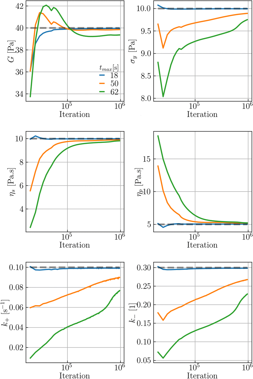
| Fig. 6 RhINN predictions using the recovered parameters for the (a and b) stress growth test at = 1 s−1 and (c and d) oscillatory shear flows at γ0 = 1 and ω = 1 rad. The first column is the normalized shear stress response, while the second one is the structure parameter response. The NN was trained using two sets of experiments; see Section 3.3. | ||
Using the recovered TEVP parameters, the MSE of the normalized shear stress, σ*, is also calculated. These MSEs in the stress growth and oscillatory shear tests are 2.8 × 10⁻¹ and 5.7 × 10⁻², respectively, using a single set of experiments. However, these MSEs reduce to 3.3 × 10⁻⁴ and 6 × 10⁻⁴ using two [or more] sets of experiments. The σ* and λ responses using the recovered parameters for both flow protocols trained with two sets of experiments are depicted in Fig. 6. The normalized shear stress and structure parameter responses closely mimic the exact values, indicating the sufficiency of only two experiments to recover the precise material response for either flow protocol. This is significant, as transient flow protocols often involve hours of pre-shearing or waiting times. Any reduction in the number of experiments can drastically reduce an experimentalist's workload, eventually leading to less material consumption with less room for human error and biases.
Moreover, the number of data points per experiment in both flow protocols (the second to last row in Table 3) was varied using two sets of experiments, and no significant improvement in parameter recovery was observed when that number was increased from 200 to 2000. This suggests that only two sets of experiments are required, relatively independent of the number of data points for each experiment, to provide an acceptable convergence. In other words, some material features are revealed only when the shear rate [or shear strain] is altered. From an experimentalist's vantage point, this finding indicates that the data resolution, provided enough sets of experiments, is likely to trivially impact parameter recovery and the subsequent accuracy of RhINNs.
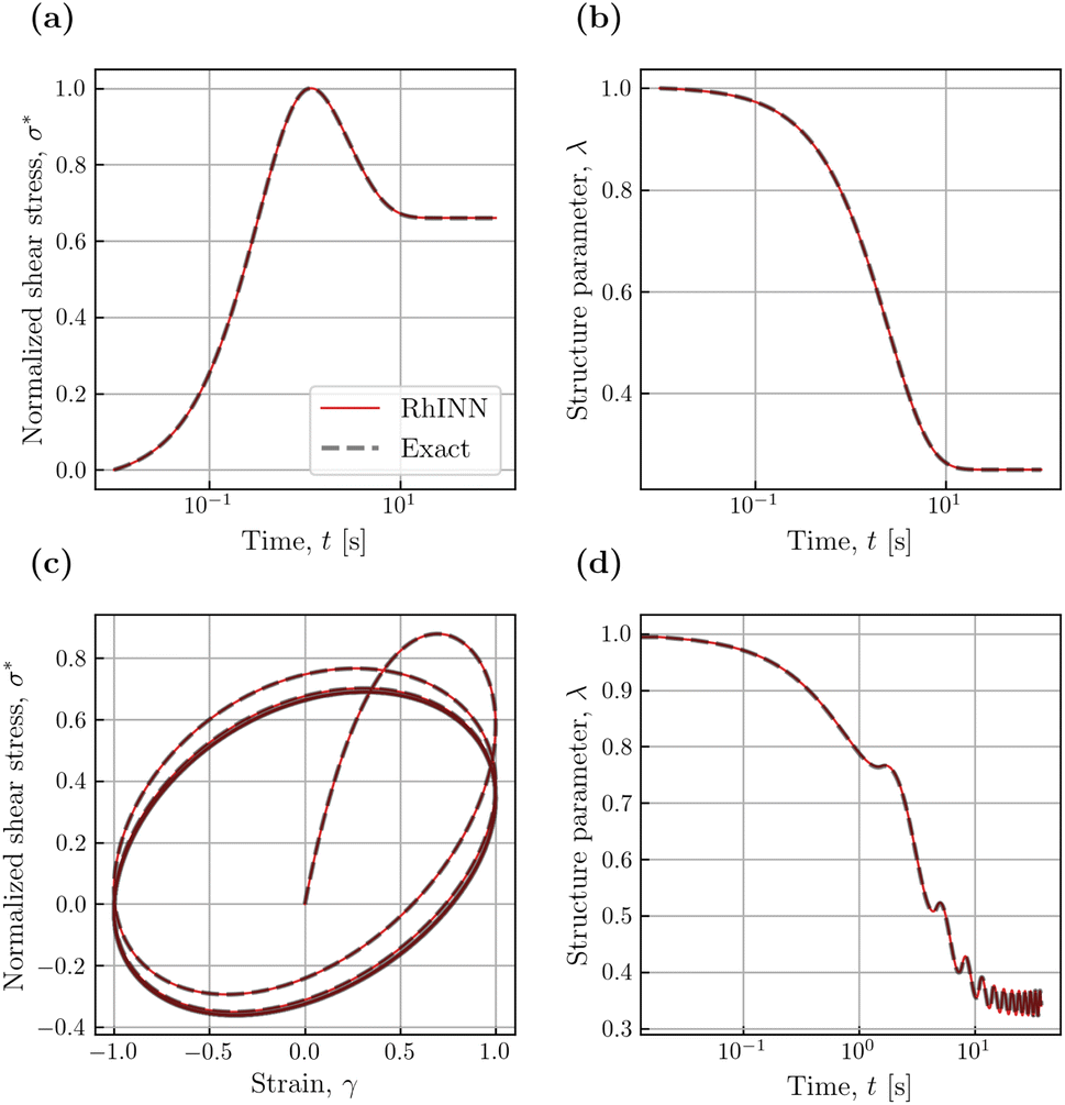
Interestingly, the selection of the observation time window, [0, tmax], has a significant impact on parameter recovery for the oscillatory shear flow. Three scenarios with time windows of [0, 18], [0, 50], and [0, 62] (in s) were considered to generate three sets of data (using five sets of experiments) while keeping all other data features (e.g., strain amplitude, frequency, and TEVP parameters) intact. Fig. 7 illustrates how the values of the six fitting parameters change during the training process. As shown, all six are accurately recovered after 5 × 10⁴ iterations using the smallest observation window, i.e., tmax = 18 s. However, some fitting parameters (e.g., σy and k−) do not converge to their respective exact values even after 106 iterations for the larger time windows of tmax = 50 and 62 s. Although for, say, k−, the parameter values for higher observation time windows may plateau [and converge] if the code is run for more iterations, it is nonetheless inconvenient to resort to higher tmax values. Instead, for the oscillatory flows, it is recommended to start with a smaller tmax, i.e., a few σ*–γ0 loops, and then gradually increase it (by simply feeding more training data in time to RhINNs) if parameter recovery is unsatisfactory, i.e., if not enough material delicacy is seen by the RhINN.
 | ||
| Fig. 7 The evolution of TEVP parameters as a function of the training iterations for various observation time windows using five sets of experiments (γ0). The gray dashed line represents the exact parameter values. For higher values of the observation time, parameter recovery is compromised. | ||
The effect of the range of original TEVP model parameters on the convergence of the recovered parameters is also explored. For this investigation, the training data for the TEVP model were generated using the stress growth test and the following parameters spanning over several orders of magnitude: G = 250 Pa, σy = 500 Pa, ηs = 500 Pa s, ηp = 5 Pa s, k+ = 0.1 s−1, and k− = 0.3. With the NN hyperparameters listed in Table 3, parameter recovery remained stubbornly elusive, and the RhINN was apparently trapped in local minima (not shown here). Efforts were made to facilitate the convergence by adjusting the NN hyperparameters and the number of data points; however, no improvement was observed. The TEVP parameters were redefined to resolve this issue, and the following ad hoc fitting parameters were introduced: G′ = G/(ηs + ηp),  ,
,  and
and  . Interestingly, it aided the convergence and ensured that all TEVP parameters were predicted within a 1% error band. Although this redefinition of parameters is performed somewhat arbitrarily and not in any form a unique solution, it does, however, assist in parameter recovery. For instance, by inverting the fitting parameters in eqn (5) and (6), the convergence may improve generally for higher values of parameters. Admittedly, parameter recovery using RhINNs is influenced by the range of unknown [actual] parameters, and several combinations of hyperparameters (e.g., heuristics and learning rates) and CM modification (e.g., parameter redefinition) should be explored to facilitate the convergence and the subsequent parameter recovery. Moreover, having prior information about one or more parameters in terms of the exact value or even the bounds of that can drastically facilitate the convergence, as discussed in detail in Section 3.1.
4 Conclusions
In this work, a rheology-informed neural network (RhINN) platform was thoroughly interrogated with respect to its ability to recover rheologically relevant parameters from a set of given flow tests. Namely, model parameters of different thixotropic elasto-visco-plastic (TEVP) constitutive models were recovered through an inverse implementation. Since the parameter space for real-world applications includes all variables of the constitutive model of choice, the neural network, and data, these different effects were systematically studied in isolation. As a practical study, we mainly focused on the interplay between three components of RhINNs that are involved in inverse problems, i.e., (i) the constitutive (TEVP) model (which is a coupled ODE system) that we wish to recover its parameters, (ii) the hyperparameters of the predictive method (RhINN), and (iii) the range and type of the given data in the form of stress growth and oscillatory shear tests. The ultimate goal is to provide reproducible, interoperable, and adaptable platforms for researchers that wish to employ RhINNs (or PINN-like algorithms in general). As such, a step-by-step study of different components within the overall framework is essential.We find that given a set of data, it is best to first gauge the complexity extent of the given data and then undertake a simple-to-complex path to select a constitutive model for that particular set of data. In other words, the complexity of the physical behavior and the model of choice should always go hand-in-hand. For instance, overly simple constitutive models that inherently cannot capture the general features of the given data are deemed to fail when embedded in the neural network as well. The neural network's physical intuition is as good as our understanding of the system and generally cannot exceed that.
When tuning the RhINN's hyperparameters to enhance parameter recovery, several key factors should be given primary attention: the learning rate, the activation function, the initial conditions, the bounds of the unknown parameters, and the error heuristics. Each of these hyperparameters may have a significant effect on the final model/material parameters recovered, and for each set of problems, these should be systematically studied before using RhINNs.
In all fairness, and not unlike similar toolboxes for tackling inverse problems, RhINNs may experience limitations in recovering parameters with irregular ranges; parameter redefinition, though, can amend this issue. Also, the execution time of RhINNs, due to their dense vectorization and rather expensive gradient-taking step, has yet to become comparable with similar techniques. However, the gap is narrowing as back-to-back NN-based calculations are becoming increasingly more efficient, with recent hardware advancements galvanizing data-driven methods. However, due to their nonlinear nature, extensive library of hyperparameters, scalability, and also ease of generalizability compared to other frameworks, RhINNs remain competitive, and for some cases, the recommended tool when tackling inverse [and forward] and ill-posed problems, with extensive research expeditiously addressing the existing limitations of physics-informed, data-driven solvers.
In rheologically relevant problems of interest, data come in different forms and through different flow protocols. Here, two transient ones were tested, and for both flow protocols, one experiment was found inadequate in properly recovering the fitting parameters. On the other hand, using two [or more] sets of experiments for either protocol ensures an accurate parameter recovery. For the oscillatory shear data, the observation time window (i.e., the number of stress–strain cycles) dramatically influenced the convergence, with higher values of the observation time window inhibiting parameter recovery. This was not the case for stress growth experiments in which, after a certain period of time, a quasi-steady state response is usually observed.
Overall, our work provides all the necessary steps to be taken before and towards employing RhINN-like algorithms for data-driven recovery of model parameters. This work was limited to a small sub-domain of potential constitutive models and a particular neural network architecture. Yet, we found that many parameters have to be considered and investigated before a rigorous and reliable data-driven model/material recovery can be performed. As such, it is essential to avoid a “one size fits all” approach and ensure a complete study of all essential components (model, network, and data) in a case-by-case manner.
Appendix
As described above, this work comprises (a) data generation using SciPy's odeint method and (b) the training process within the neural net. To further facilitate the implementation in any programming language, the pseudo-codes for these two steps (assuming the stress growth flow protocol) are provided in Algorithms 1 and 2, respectively.
|
|
Data availability
All the codes and data used in this study are publicly available on the group’s GitHub repository at https://github.com/procf/RhINNs.Conflicts of interest
The authors declare that there is no conflict of interest.Acknowledgements
The authors acknowledge the National Science Foundation's DMREF #2118962 award.Notes and references
- R. Larson and P. S. Desai, Annu. Rev. Fluid Mech., 2015, 47, 47–65 CrossRef.
- F. A. Morrison, Understanding rheology, Oxford University Press, New York, 2001, vol. 1 Search PubMed.
- C. W. Macosko, Rheology : principles, measurements, and applications, VCH, 1994, p. 550 Search PubMed.
- R. B. Bird, R. C. Armstrong and O. Hassager, Dynamics of Polymeric Liquids, Volume 1: Fluid Mechanics, Wiley-Interscience, 1987 Search PubMed.
- E. C. Bingham, Bull. Bur. Stand., 1916, 13, 309–353 CrossRef.
- W. H. Herschel and R. Bulkley, Kolloid-Z., 1926, 39, 291–300 CrossRef.
- C. J. Dimitriou and G. H. McKinley, Soft Matter, 2014, 10, 6619–6644 RSC.
- P. R. de Souza Mendes, Soft Matter, 2011, 7, 2471 RSC.
- M. J. Armstrong, A. N. Beris, S. A. Rogers and N. J. Wagner, J. Rheol., 2016, 60, 433–450 CrossRef CAS.
- Y. Wei, M. J. Solomon and R. G. Larson, J. Rheol., 2016, 60, 1301–1315 CrossRef CAS.
- R. G. Larson, J. Rheol., 2015, 59, 595–611 CrossRef CAS.
- R. G. Larson and Y. Wei, J. Rheol., 2019, 63, 477–501 CrossRef CAS.
- S. Jamali and G. H. McKinley, J. Rheol., 2022, 66, 1027–1039 CrossRef CAS.
- M. Agarwal, S. Sharma, V. Shankar and Y. M. Joshi, J. Rheol., 2021, 65, 663–680 CrossRef CAS.
- J. Mewis and N. J. Wagner, Adv. Colloid Interface Sci., 2009, 147–148, 214–227 CrossRef CAS PubMed.
- C. F. Goodeve and G. W. Whitfield, Trans. Faraday Soc., 1938, 34, 511 RSC.
- D. E. White, G. D. Moggridge and D. I. Wilson, J. Food Eng., 2008, 88, 353–363 CrossRef.
- T. M. Inc., MATLAB, 2022 Search PubMed.
- E. Jones, T. Oliphant, P. Petersonet al., SciPy: Open source scientific tools for Python, 2001 Search PubMed.
- I. W. Research, Mathematica 13.2, 2022 Search PubMed.
- J. W. Eaton, D. Bateman and S. Hauberg, GNU Octave version 3.0. 1 manual: a high-level interactive language for numerical computations, SoHo Books, 2007 Search PubMed.
- A. D. Jagtap, Z. Mao, N. Adams and G. E. Karniadakis, arXiv, 2022, preprint, arXiv:2202.11821, https://arxiv.org/abs/2202.11821 Search PubMed.
- Y. Chen, L. Lu, G. E. Karniadakis and L. D. Negro, Opt. Express, 2020, 28, 11618 CrossRef PubMed.
- M. Raissi, P. Perdikaris and G. Karniadakis, J. Comput. Phys., 2019, 378, 686–707 CrossRef.
- G. E. Karniadakis, I. G. Kevrekidis, L. Lu, P. Perdikaris, S. Wang and L. Yang, Nat. Rev. Phys., 2021, 3, 422–440 CrossRef.
- M. Raissi, A. Yazdani and G. E. Karniadakis, Science, 2020, 367, 1026–1030 CrossRef CAS PubMed.
- M. Raissi, J. Mach. Learn. Res., 2018, 19, 932–955 Search PubMed.
- P. Karnakov, S. Litvinov and P. Koumoutsakos, arXiv, 2022, preprint, arXiv:2205.04611, https://arxiv.org/abs/2205.04611 Search PubMed.
- Z. Li, K. Meidani and A. B. Farimani, arXiv, 2022, preprint, arXiv:2205.13671, https://arxiv.org/abs/2205.13671 Search PubMed.
- S. Cai, Z. Mao, Z. Wang, M. Yin and G. E. Karniadakis, Acta Mech. Sin., 2022, 1727–1738 Search PubMed.
- Z. K. Lawal, H. Yassin, D. T. C. Lai and A. C. Idris, Big Data Cogn. Comput., 2022, 6, 140 CrossRef.
- M. Mahmoudabadbozchelou and S. Jamali, Sci. Rep., 2021, 11, 12015 CrossRef CAS PubMed.
- M. Mahmoudabadbozchelou, M. Caggioni, S. Shahsavari, W. H. Hartt, G. E. Karniadakis and S. Jamali, J. Rheol., 2021, 65, 179–198 CrossRef CAS.
- M. Mahmoudabadbozchelou, G. E. Karniadakis and S. Jamali, Soft Matter, 2022, 18, 172–185 RSC.
- M. Mahmoudabadbozchelou, K. M. Kamani, S. A. Rogers and S. Jamali, Proc. Natl. Acad. Sci., 2022, 119, e2202234119 CrossRef CAS PubMed.
- M. Saadat, M. Mahmoudabadbozchelou and S. Jamali, Rheol. Acta, 2022, 721–732 CrossRef CAS.
- J. B. Freund and R. H. Ewoldt, J. Rheol., 2015, 59, 667–701 CrossRef CAS.
- M. J. Armstrong, A. N. Beris and N. J. Wagner, AIChE J., 2017, 63, 1937–1958 CrossRef CAS.
- P. K. Singh, J. M. Soulages and R. H. Ewoldt, Rheol. Acta, 2019, 58, 341–359 CrossRef CAS.
- S. Thakur, M. Raissi and A. M. Ardekani, arXiv, 2022, preprint, arXiv:2301.13262, https://arxiv.org/abs/2301.13262 Search PubMed.
- B. Reyes, A. A. Howard, P. Perdikaris and A. M. Tartakovsky, Phys. Rev. Fluids, 2021, 6, 073301 CrossRef.
- P. R. de Souza Mendes and R. L. Thompson, J. Non-Newtonian Fluid Mech., 2012, 187–188, 8–15 CrossRef CAS.
- S. Jamali, G. H. McKinley and R. C. Armstrong, Phys. Rev. Lett., 2017, 118, 048003 CrossRef PubMed.
- A. G. Fredrickson, Principles and applications of rheology, Prentice-Hall, 1964 Search PubMed.
- J. S. Horner, M. J. Armstrong, N. J. Wagner and A. N. Beris, J. Rheol., 2019, 63, 799–813 CrossRef CAS.
- P. R. de Souza Mendes, B. Abedi and R. L. Thompson, J. Non-Newtonian Fluid Mech., 2018, 261, 1–8 CrossRef CAS.
- M. Geri, R. Venkatesan, K. Sambath and G. H. McKinley, J. Rheol., 2017, 61, 427–454 CrossRef CAS.
- M. J. Armstrong and A. M. Pincot, Open J. Fluid Dyn., 2022, 12, 36–55 CrossRef.
- J. Blechschmidt and O. G. Ernst, GAMM Mitt., 2021, 44, e202100006 Search PubMed.
- M. Saadat, demang89 and D. Dabiri, procf/RhINNs: Version 1.0.0 (v1.0.0), 2023 Search PubMed.
Footnotes |
| † By limiting ourselves to shear flows and overlooking extensional flows, important insights into a material's full response are indeed relinquished. However, due to the shortage of extensional rheometry [and subsequent data] in the literature, the limited endeavors on model development for extensional flows seem less conspicuous, at least for now. |
| ‡ https://github.com/procf/RhINNs |
| § https://github.com/procf/RhINNs |
| ¶ This is rather important, as the scientific community is deeply influenced by The Hitchhiker's Guide to the Galaxy and the “Answer to the ultimate question of life, the universe, and everything.” |
| || Activation functions on TensorFlow: https://www.tensorflow.org/api_docs/python/tf/keras/activations |
| This journal is © The Royal Society of Chemistry 2023 |