Uncertainty-aware and explainable machine learning for early prediction of battery degradation trajectory

Abstract

Enhancing cell lifetime is a vital criterion in battery design and development. Because lifetime evaluation requires prolonged cycling experiments, early prediction of cell aging can significantly accelerate both the autonomous discovery of better battery chemistries and their development into production. We demonstrate an early prediction model with reliable uncertainty estimates, which utilizes an arbitrary number of initial cycles to predict the whole battery degradation trajectory. Our autoregressive model achieves an RMSE of 106 cycles and a MAPE of 10.6% when predicting the cell's end of life (EOL). Beyond being a black box, we show evidence through an explainability analysis that our deep model learns the interplay between multiple cell degradation mechanisms. The learned patterns align with existing chemical insights into the rationale for early EOL despite not being trained for this or having received prior chemical knowledge. Our model will enable accelerated battery development via uncertainty-guided truncation of cell cycle experiments once the predictions are reliable.

---

1 Introduction

The deployment of lithium-ion batteries is expected to grow dramatically over the next decade as the transportation sector becomes electrified and grid-level battery storage becomes more commonplace to balance fluctuating renewable energy sources. Designing batteries with a longer cycle life leads directly to better economics¹ and a lower carbon/environmental footprint from mining and manufacturing.² The capacity of a secondary (rechargeable) battery cell degrades over its lifetime and for many practical purposes, the failure threshold is considered to be when the battery capacity falls below 80% of the nominal capacity, which is called the cycle life.^3,4 After this point, capacity degradation tends to progress at a much faster rate and therefore the cell needs to be replaced.⁵ The cycle life of a cell depends on the usage scenarios, internal chemical, and structural details,⁶ which can vary significantly even between cells manufactured from the same production line. However, the process of optimizing batteries (materials and cell design parameters) for improved cycle life is hindered by a slow lifetime evaluation process. Being able to accurately determine the lifetime of the battery with limited early-cycle data would enable us to fast forward the battery development cycle.

The cycle life of a battery is strongly dependent on how it is operated, e.g. the charging C-rate, temperature, or cut-off voltage, as these conditions determine the incidence of deleterious electrochemical side reactions in the anode, electrolyte, and cathode. Balancing between longer cycle life and faster charging time is a major engineering challenge in making electric vehicles (EV) a competitive alternative to conventional cars. Designing charging schedules to achieve this goal can be extremely time consuming, as testing typically extends months before observing any effect that the design has on cell cycle life. Early prediction of cycle life would significantly expedite such testing and thus enable the design of smarter charging schedules that extend battery life.⁷ Early prediction of degradation would also support the design of advanced battery management systems (BMS). Since battery performance at the pack level deteriorates when cells operate in heterogeneous states of health,⁸ an early prediction model would grant the BMS control over individual cells based on their specific degradation trajectory and thus warrant significant lifetime improvements at the battery pack level.⁹

Accurate prediction of battery lifetime is challenging because each cell undergoes complex electrochemical processes during operation, and cycling is associated with non-linear degradation.¹⁰ Physics-based modeling of battery degradation that captures a plethora of multi-time/length-scale electrochemical and mechanical processes would be prohibitively expensive. Instead, parametric models (e.g. P2D (Pseudo-Two-Dimensional) or single particle) approximate cell degradation using simpler governing equations, with a limited ability to capture complex interactions between degradation mechanisms. Data-driven models have recently been able to overcome cost-accuracy trade-offs in this task by learning high-dimensional correlations among system-level observables that might implicitly represent internal electrochemical processes. Recently, hybrid physics and machine learning models, and physics and uncertainty-aware machine learning models have been envisioned as the future direction of research.^11,12

Most data-driven models of cell degradation use online data¹³ (battery state of health up to the point of prediction) to predict near-term behavior,^14–16 but do not model early prediction (lifetime behavior from early cycles). Furthermore, most of the published work does not consider the variabilities encountered between similar types of cells^14,17 (even of the same chemistry and design). Pioneering work by Severson et al.¹⁰ followed by two other articles^18,19 has showcased different approaches towards data-driven early degradation prediction considering intra-chemistry variance.

Using hand-engineered features that incorporate domain knowledge, Severson et al.¹⁰ trained a linear regression model with elastic net regularization to predict the total lifetime of the battery cell. The model does not consider uncertainty over the output, making it hard to detect when the battery is outside the training distribution or the prediction is otherwise unreliable. With a dilated CNN (Convolutional neural network) model, Hong et al.¹⁹ predicted the remaining useful lifetime based on in-cycle time series data from the early cycles. Although this model provides an uncertainty estimate for the EOL it does not predict the entire degradation trajectory, rendering the model uninterpretable in regard to the degradation mechanisms. The work from Strange and Dos Reis²⁰ uses a CNN to predict the knee point, the knee onset point, and the EOL based on extensive data from a single cycle. These points are used to reconstruct the entire capacity degradation trajectory with a combination of a straight line and a cubic spine. In contrast to our work using deep ensembles to obtain uncertainty, they use Dropout, a technique to regularize neural networks, to approximate uncertainty over the output.²¹ Saxena et al.²² in similar work used a CNN to predict four distinct points, including EOL, on the capacity degradation trajectory and used these to construct a parameterized capacity degradation trajectory.

Li et al.¹⁸ with a sequence-to-sequence LSTM (Long Short-Term Memory neural network) recently predicted the full degradation trajectory. Gaussian process regression (GPR) has been used to detect battery failure.¹⁶ Jiang et al.²³ have employed an uncertainty-aware Hierarchical Bayesian Model (HBM) to predict the quality of a battery cycling protocol independent of the intra-chemistry variance between batteries cycled with the same protocol and only focused on lifetime. In another very recent work, Paulson et al.²⁴ used an extensive feature selection process, considering 396 features, to predict the battery lifetime for a multi-chemistry dataset.

However, no existing model can predict full degradation trajectories with uncertainty estimates both in and out of distribution (both near and far from training data distribution) ideally capturing both epistemic and aleatoric uncertainties. Having uncertainty estimates allows us to e.g. recognize when a prediction is unreliable because the data point lies too far from the training distribution and perform on-the-fly control of how much cycling is done. The prediction of a full trajectory helps to understand the causation of degradation. Learning a universal function of how cells degrade across cell chemistries requires an expressive and complex model.²⁵

Uncertainty-aware, predictive, explainable, and flexible models to predict battery degradation also represent essential building blocks to accelerate the development of new sustainable high-performance batteries.^25–27 More specifically, the ability to predict the EOL and degradation trajectory of any cell from its initial cycles would shrink the costs/time of experimentally testing the cell for hundreds of cycles; such a model would effectively accelerate the search for promising battery chemistries. Battery research acceleration would greatly benefit from models capable of making accurate and certain predictions on cells similar to those used for training, already from a low number of initial cycles. However, such models must be aware when they are wrong, i.e. they should express high uncertainty when, for instance, they attempt to make predictions on cells with significantly different chemistry (e.g. new electrolyte formulation). In addition, if these models are explainable, they would enable scientists to gain insight into the degradation mechanism, and thus have trustworthy models that are able to extrapolate. However, achieving model expressiveness that allows the learning of different degradation mechanisms purely from easy-to-access data across cell formats and cell chemistry requires complex deep learning models, which thwart understanding of how the model learns.

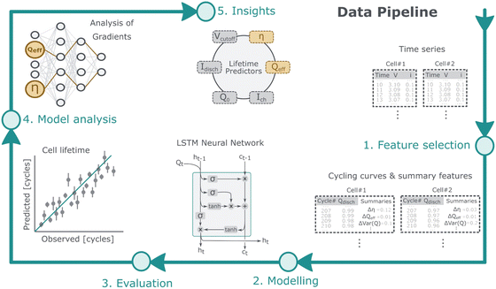
Although recently published models cover one or the other of these desirable aspects, none of them can serve the purpose of an acceleration platform for autonomous battery development. So we focused on developing a model that can be trained with different chemistries/formats, can handle varying cycling parameters, display uncertainty over the prediction, and can adjust the trajectory roll-out on the fly while being explainable. Toward this challenge, our contributions can be summarized as such (Fig. 1):

Fig. 1 Schematic overview of the prediction process.

• We introduce a deep recurrent neural network architecture (LSTM) that can be trained to predict future capacity and EOL (End of Life) without requiring insight into the battery chemistry. It can be trained with datasets of different battery chemistries.

• The trained model outputs a complete degradation trajectory that includes not only the mean but also the variance, allowing for uncertainty-aware prediction. Ensemble models are built in addition to the uncertainty as a direct model output.

• We evaluated this architecture on available battery datasets, showing that it outperforms multiple competitive baselines. We also show how robust uncertainty capability allows the model to adjust input cycle information on the fly to lower uncertainty.

• We consider the explainability of the trained model on LFP battery data. Our findings show, among other things, that the LSTM model recognizes qualitative differences between short- and long-lived batteries. The model gradient differences are aligned with prior understandings about degradation mechanism and open up the possibility of an easy way to predict main degradation mechanisms.

To the best of our knowledge, our model is the first one that can model the entire capacity fade trajectory from the early cycles without a fixed limit on the maximum lifetime. Using an LSTM allows us to visualize the influence of different inputs over the lifetime of the battery and draw insights from the data-driven model.

We show preliminary results on openly available but limited cycling datasets from commercial cells using nickel cobalt aluminum oxide (NCA) and nickel manganese cobalt oxide (NMC) as positive electrodes. While the architecture itself is chemistry neutral, i.e. not restricted to use on a specific chemistry, it requires a dataset of batteries with the specific chemistry that we want to predict capacity for. Models that can simultaneously predict capacity for f.e. LFP, NCA and NMC batteries at the same time would require a dataset that allows generalizing over chemistries by including batteries with different chemistries that were cycled under comparable conditions. We leave this work to future research.

2 Methods

2.1 Data resources

For this work, we used a previously available battery cycling dataset.¹⁰ The reader is referred to the original publication for more detailed information. The dataset originally consisted of 135 commercial LFP/graphite cells, each with a nominal capacity of 1.1 A h and cycled in a temperature controlled chamber at 30 °C. Each cell was operated at one of 72 different fast-charging protocols.

The charging schedule for each cell was a one- or two-step policy from 0% to 80% SOC followed by a uniform 1 C CC-CV charging step to 3.6 V for all cells. For the two-step policies, the point at which the charging protocol was changed is varied between 0% and 80%. Discharging was identical for all cells at 4 C to 2.0 V.

Varying the charging conditions resulted in a wide range of cycle lifetimes, ranging from 150 to 2300 cycles. The dataset was partitioned into three batches for cycling by Severson et al.¹⁰ Each batch was cycled inside the chamber under different testing conditions and on different dates. In the original paper, the first two batches are used for training and validation, while the third batch was used for testing. We removed cells with experimental errors, as suggested by the authors in their published code, resulting in 124 useable cells.¹⁰

Since the three batches of cells were cycled at different times, they underwent calendar aging for different amounts of time. Severson et al.¹⁰ note in the supplements that the third batch was calendar-aged for approximately a year longer than the first two batches. Since calendar aging influences the capacity of a battery, ML algorithms that were trained only on data from non-calendar-aged batteries will perform worse when predicting the future capacity of calendar-aged batteries (and vice versa). As the training data consist only of data from non-calendar-aged batteries, we break down the performance into the prediction of calendar-aged and non-calendar-aged data separately. We stress that the model we used to report performance on the calendar-aged cells is only trained on non-calendar-aged batteries. In comparison to being trained on a combination of non-calendar-aged and calendar-aged data, this is a harder task for an ML algorithm to solve.

The first two batches consisting of non-calendar-aged battery cells were used for training, validation, and testing in our work, while the third batch was used to test the model performance on calendar-aged cells. To do this, we randomly split up the first two (non-aged) batches of the dataset into 50% training data and 25% each for validation and testing. For clarity, the data split is visualized in Fig. S8 in the ESI.† The performance in the test data is reported in the first columns of Table 1. The performance in the calendar-aged batteries of the third batch is reported separately in the second column of Table 1. In the supplements we show additional results on a dataset of 40 cells with NMC and NCA chemistry (22 NMC, 18 NCA) published by the Sandia National Labs.²⁸

Table 1 RMSE prediction error for the number of cycles on the prediction of EOL for baselines and LSTM based on the first hundred cycles

	Non-aged batteries	Calendar aged batteries
a Direct prediction of the total lifetime.
Linear regression^a	151	202
LSTM (ensemble)	106	184
LSTM	172	243
DNN (no capacity)	207	402
LSTM (no covariates)	587	384

---

Inconsistency in data generation and insufficient documentation presented a large issue when choosing datasets for this work. For example, testing cycles were often not annotated, and many datasets contained several discontinuities such as outliers and unexplained steps in capacity (examples are shown in Fig. S2†). The general quality of the data presented an issue when finding datasets for this work. For one, measurement inconsistencies meant that not all cells reported the voltage profiles necessary to calculate battery-specific but time-independent features hereafter referred to as covariates. Often, degradation trajectories showed outliers or unexplained jumps in capacity (examples are seen in Fig. S2†) which, without appropriate annotation, cannot be automatically removed or imputed. As in any other field of research, the development and testing of new machine learning models for cell degradation is limited by the amount and quality of available data. There are many different approaches to handling missing and noisy data. The best approach for a given case depends among other things on the knowledge about the data collection process and the amount of domain expert person hours available. Since the dataset did not include annotations for frequent outliers and jumps, we had to rely on heuristics to impute them.

2.2 Data processing

For each cell, we use an input trajectory, i.e. the degradation trajectory up to an arbitrarily chosen number of initial cycles, as the basis for predicting the full degradation trajectory. For instance, an input trajectory of 30 cycles Q[0−30] uses the degradation trajectory of the first 30 cycles to predict the remaining trajectory until the EOL. We report results for a range of input trajectories from 20 to 100. Reporting for this wide range of initial cycles starting at a low number of twenty (chosen ad hoc as the starting point) allows us to analyze the number of initial cycles needed to reach a specific accuracy for the EOL prediction. It also highlights the flexibility of the model in terms of the initial cycles available. As can be seen from the results in Fig. 5, the RMSE quickly levels off as more initial cycles become available.

For network training, we used the degradation trajectory, that is, (a) the discharge capacity trajectory vs. cycle, (b) the charging schedule and (c) a set of three covariates described in Section 2.5 where we also extend the selection process for the variables chosen. We preprocessed the data by removing obvious outliers and replacing them with the mean value over the dataset. Subsequently, we standardized the covariates to have a mean of zero and a variance of one. We also use the logarithm of the current cycle number as a supplementary covariate. This does not contain information on the internal state of the battery itself. However, in practice, we found that this improves the training process for the prediction of EOL because it facilitates an easier comparison of how quickly the capacity degrades.

To calculate the variance between capacity–voltage curves, we follow Severson et al.¹⁰ and fit the discharge capacity as a function of the voltage, which is evaluated at 1000 linearly spaced points between 2 and 3.5 volt. We calculate the variance between the resulting vectors for the tenth cycle and the last input cycle. The charging schedule of each cell is expressed as a three-dimensional vector containing the minimum, maximum, and average charging rate throughout the cycling for the LFP dataset.

The discharge capacity at every cycle Q_n (the subscript denotes the cycle number) is predicted as the remaining proportion of the capacity in the previous cycle. Degradation trajectories often contain a substantial amount of noise. For the target (the next cycle capacity) during model training we, therefore, preprocess the capacity trajectories for training with a simple moving average filter (MAF) over twenty cycles centered around the current cycle.

2.3 LSTM architecture

We use an LSTM to process the capacity trajectories.²⁹ In an extension of a traditional neuron, an LSTM neuron contains a memory state that is updated at each time step. Time sequences such as the capacity trajectory are fed into the LSTM neural network concurrently. For multistep prediction, the predicted output is appended onto the input to create the next input. The proposed NN consists of one LSTM layer, one fully connected hidden layer, and one fully connected output layer to predict the loss in capacity in the current cycle based on previous capacities as shown in Fig. S1.† To choose the optimal number of neurons, cross-validation was performed, resulting in 32 neurons for each layer.

To capture uncertainty, instead of predicting a single value, our NN outputs both the predicted mean capacity at the next step y_pred and its expected variance σ²; the variance allows us to express uncertainty in the prediction. To train the NN we use a common approach, minimizing the negative log-likelihood (NLL) as a loss function over the Gaussian distribution output by the NN and the true next step value.^30,31 With the NN outputting the mean y_pred and variance σ² this is

ŷ is the true value at the next step. This corresponds to maximizing the probability that the true value of the next step comes from the probability distribution predicted by the NN.

When predicting the trajectory for a new battery, we obtain the next time step value by sampling from a Gaussian distribution with the predicted mean and variance. Since we are interested in obtaining uncertainty over the entire trajectory, we sample multiple independent trajectories from each NN in the ensemble during test time. For each trajectory, we concurrently obtain the next time step in the manner just described until the predicted trajectory reaches its EOL. The mean and variance of the time step t for K neural networks in the ensemble with L trajectories sampled from each become

The NN was trained with the Adam optimizer with the default learning rate of 0.001.³² Training is stopped once validation loss no longer improves for three concurrent epochs. During testing, it is required to roll out multiple capacity trajectories to obtain an accurate measure of the uncertainty over the output. We use an ensemble of five neural networks (trained with different random seeds) and sample ten trajectories from each network. During the roll-out, we concurrently sample the next value in the capacity trajectory from the output mean and variance predicted by the neural network in the current step. The trajectories of all neural networks in the ensemble are concatenated, and the distribution of trajectories is calculated.

Unless otherwise noted, all performance metrics are averaged over five random seeds. All experiments were carried out with PyTorch on a Nvidia RTX 3090.³³ The code used to process the datasets, train the models, and create the results presented in this study will be released on acceptance.

2.4 Saliency analysis

To analyze how important input parameters change during trajectory prediction, we apply a saliency analysis to the LSTM on the test data. Neural networks are trained with gradient descent, i.e. computing the gradient of the loss function over the weights and taking a step in the negative direction. We use a similar approach and take the absolute gradient of the output over the input. Intuitively, this highlights input dimensions where a slight change in the input will result in a large change of the output.

To be able to compare different batteries and cycles, we normalize these values so that the gradients for one cycle always sum up to one. By taking the average importance of the inputs over different subsets of batteries and cycles, we can extract information about the general importance of, e.g. the coulombic efficiency for prediction. We discuss the results in Section 3.5.

2.5 Feature selection

The objective of the ML algorithm is to predict the lifetime of LiFePO/graphite cells from a given number of initial cycles. Accordingly, we train the algorithm with cycling trajectories (i.e., discharge capacity vs. cycle) and a set of additional electrochemical features from the initial cycles. These features are selected based on being both (i) informative, i.e. known to be correlated with cell lifetime, (ii) accessible, i.e. available from most common cycling experiments, and (iii) able to generalize between experiments. For example, while cycling temperature affects capacity fade, we disregard it as a feature because the impact of temperature is highly dependent on, e.g., the temperature of the environment and the form factor of the cell. For ML algorithms, it is important that features generalize across datasets. This means that the correlation between input and output should be consistent between batteries and datasets. Using temperature as an example, an increase in temperature could mean that e.g. the core temperature of the cell had increased or that the environment temperature had increased. Since the model cannot distinguish these two different scenarios from each other on the basis of the temperature, the temperature cannot be used to infer information about the cell SOH.

Hence, incorporating temperature as a feature in the model restricts its ability to generalize to other cell designs and environments. Therefore, we choose to exclude temperature as a feature, since it is also indirectly represented in the variables that we include.

The cycling charge rate affects the degradation of LiFePO4/graphite cells^34–36 and is always recorded in cycling experiments; therefore, we include the maximum, minimum, and mean charging rate as features to account for cycling conditions. The discharge rates might also be considered, but we do not use them because all cells in the dataset are discharged at the same rate.¹⁰ In addition to the charging rates, we select three electrochemical metrics as features. Coulombic efficiency, charge–discharge voltage gap, and differential capacity trajectories reflect the loss of active Li+, the build-up of internal resistance, and the electrochemical reaction mechanisms of a cell during a cycle, respectively.^37–39 Given that the coulombic efficiency is a scalar value, it can be used directly as a feature. On the other hand, the voltage gaps and the differential charge curves are voltage- (or state-of-charge)-dependent vectors that need to be encoded as single scalar features per cycle. As a simple approximation, we describe the voltage gap as the difference between the mean voltage during charge and the mean voltage during discharge. Finally, we inherit the differential charge curve feature engineered from Severson et al.,¹⁰ who demonstrated that the variance of the difference between the charge and discharge capacity vectors was well correlated with the cell lifetime.¹⁰

Using 6 features for every cycle would result in hundreds of inputs to characterize the degradation behavior of a single cell, which is impractical. Training on more features than examples would render the model not only larger, but also ill-posed to generalize. Fortunately, these features vary very little from cycle to cycle for a single cell, so it is sufficient to summarize them by their variations within the initial cycles. For consistency with Severson et al.,¹⁰ we use the feature difference between the 10th cycle and the last cycle m available for prediction, represented as X_m−10. In the following, we refer to these battery cell-specific, time-independent features as covariates, which are described in Table S1† and illustrated in Fig. S6.†

In addition to being readily accessible from electrochemical time series, we believe that these features implicitly capture (i) the influence of uncontrolled experimental conditions (e.g., cell manufacturing, geometry, preconditioning) and (ii) the cell's state of health during cycling independently of the chemistry of the electrodes. Chemistry-neutrality ensures that the features can be readily used to train on datasets from other cell chemistries and pave the way for high-accuracy chemistry-neutral models to predict degradation with additional data.

3 Results

3.1 LSTM performance compared to baseline models

LSTMs are well suited for modeling sequential data as they do not have constraints on the total time series length and can model complex correlations and features in sequential data streams. As such, they are a popular choice for modeling time series as we want to do here. Since the entire capacity trajectory is predicted, they also allow us to examine, e.g., when the capacity starts degrading rapidly.

To demonstrate the advantage of LSTM operating with electrochemically inspired features, we compare the LSTM with three baselines, a linear regression (LR) with elastic net regularization based only on covariates (inspired by and similar to Severson et al.¹⁰), a Dense Neural Network (DNN) based only on the covariates, and an LSTM based only on the capacity trajectory. In contrast to neural networks, the LR model can only estimate the End of Life (EOL) but can not model the complete capacity trajectory. Furthermore, we compare our approach to values taken from the literature in Table 2 and refer to Ng et al.³ and Lv et al.⁴⁰ for an extensive overview. For the resulting metrics in Table 2 it should be noted that they are taken on different training/validation/test splits of the data and therefore are not directly comparable.

Table 2 RMSE and MAPE prediction for our model vs. values taken from literature^a

	RMSE	MAPE
a The performance metrics are all for different data splits of the dataset introduced in Severson et al.^10 and not directly comparable.
LSTM ensemble (ours)	106	10.6%
Severson et al^10	173	8.6%
Strange and Dos Reis^20	110	8.8%
Ma et al^41	76	9.0%

---

To compare our modeling approaches with linear regression, we report the RMSE (Root Mean Square Error) on the predicted total lifetime in Table 1. The RMSE is calculated as

N refers to the total number of cells. y_n and y_n,pred refer to the actual and predicted lifetimes of the n_th cell respectively.

The results show that an ensemble LSTM (comprised of five NN initialized with different random weights) has a lower Root Mean Square Error (RMSE) when predicting the EOL than the neural network baselines and the LR, indicating that it better captures the relationship between cycling patterns within the first few cycles and the total lifetime. In addition to the MAPE of 10.6%, our model has an MAE of 76.5. Unlike previous work,¹⁰ we separately evaluated the prediction performance on calendar-aged and non-calendar-aged batteries as we found significant differences in the behavior of the battery cells depending on their storage history (see Fig. S4†).

Calendar-aged cells seem to last longer compared to non-aged cells under the same cycling conditions. Prolonged storage of cells might influence, for instance, electrode passivation in a way that results in improved lifetime compared to non-aged cells, similar to formation cycles.⁴² Consequently, the model struggles to predict the degradation of aged cells which it has not seen during training.

Notably, the improvement in predictive performance also holds for calendar-aged batteries. In Table 1 we see that the ensemble LSTM is more accurate in predicting EOL for calendar-aged batteries, as indicated by the lower RMSE, implying that some of the chemical processes that occur during calendar aging are implicitly captured in the early cycles as well and are learned by the LSTM.

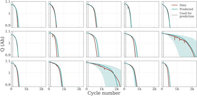
To show that in addition to accurate EOL prediction, our model also matches the capacity trajectories, we show capacity trajectories on the test set of non-calendar-aged batteries in Fig. 3. We provide capacity trajectory predictions for calendar-aged batteries in Fig. S6.† In contrast to only predicting EOL, modeling the entire capacity trajectory allows detailed analysis of the degradation pattern and helps us gain an understanding of possible electrochemical phenomena causing it. The LSTM ensemble matches the actual trajectory closely, accurately predicting the knee point, i.e. the cycle number where the trajectory visibly bends, to an accelerated degradation. Calculated over the true lifetime, the LSTM ensemble has an R² value of 0.765 for predicting the trajectories compared to the observed trajectories.

3.2 Capturing uncertainty

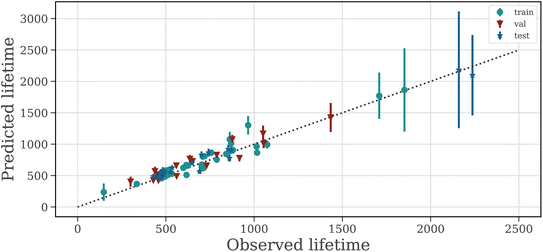
Highly parameterized deep learning models like ours are prone to fail when generalizing to datasets that are very dissimilar to the dataset that the model is trained with, such as new battery chemistries or aging processes that dramatically alter the degradation pattern. The trustworthiness of the model can be questioned if the model is overconfident in its predictions i.e. it does not know when it is wrong. In Fig. 3, we show the uncertainty of the output trajectory (the shaded area in Fig. 3 encompasses the 5th to the 95th percentile). Information about the certainty of the prediction is important for risk assessment during model deployment and can be used for active learning based data collection from experiments.

For most batteries, the uncertainty over the trajectory is low. Notably, two batteries in the test set have a lifetime beyond any lifetime seen in the training set. The predictions for these batteries are associated with a high uncertainty over the capacity trajectory and EOL. The results in Fig. 2 show that the uncertainty over the EOL is low for batteries with a lifetime of up to 1000 cycles (as expected given that the majority of battery cells in the training data set lie in this range) and high above that. This is expected and desired behavior, as the ML model has less information about the data distribution in this range.

Fig. 2 LSTM ensemble prediction vs. ground truth based on 100 cycles. Error bars indicate SD.

Fig. 3 Predicted trajectories of unseen batteries. Prediction is the 50th percentile, the shaded area is the uncertainty estimate (from the 5th to the 95th percentile). For the two batteries with a higher lifetime than any battery seen in the training set, the uncertainty is high.

In Fig. 4 we show quantitatively what percentage of observed trajectories are included in a respective quantile as predicted vs. as observed. Ideally, this line should be close to the identity function. The model is still slightly overconfident as can be observed from the slope but the error is well correlated with the uncertainty.

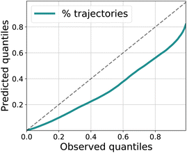Fig. 4 Evaluation of uncertainty for the trajectories. We plot the predicted quantiles as a function of the observed quantiles. The LSTM ensemble is slightly overconfident in its predictions.

In Fig. S4† we show example trajectories for the calendar-aged batteries. The model predicts comparatively higher uncertainty over the trajectory for aged cells. Since the predictions become more uncertain on the trajectories of aged cells, we conclude that our model has learned data patterns – possibly electrochemical signatures – differentiating aged from non-aged cells.

3.3 How early can we predict with how little data?

Getting accurate information about the future degradation pattern of a battery early in its life is vital. Each potential application of our model might require a different trade-off balance between the accuracy of prediction and how much cycling data the model would need as input. We characterize such trade-offs by evaluating how the accuracy of our algorithm changes with the number of cycles input into the neural network in Fig. 5.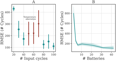

Fig. 5 (A) Accuracy of LSTM ensemble plotted against the number of cycles used as input. The error bars indicate SD. According to ref. 10 there was a temperature aberration in the test chamber around 55 and 70 cycles, causing a larger error for 50, 60, and 70 cycles. (B) Accuracy of LSTM plotted against the number of batteries used for training. The shading indicates SD. For accurate learning, only a small number of batteries is needed.

The accuracy of prediction (in terms of RMSE in the test data) improves as more of the initial cycling data is used as input to the model, as shown in Fig. 5. With a larger part of the degradation trajectory visible, forecasting future degradation becomes easier as more information about the degradation process becomes available. Additionally, the results in Fig. 5 show that the error decreases rapidly with as few as thirty cycles available, demonstrating that the LSTM can robustly predict the EOL early in the lifetime; more specifically, the model predicts the EOL with an RMSE of 173 cycles using only the first 40 cycles of the trajectory.

Testing conditions such as operating temperature directly affect the internal electrochemistry of the battery. Fluctuations in these variables, if not taken into account during modeling, can cause larger errors. Even if our model is not trained while using temperature as a predictor, it still captures some of these effects implicitly through other covariates and has a high level of accuracy when it is trained on data with and without those aberrations (e.g. predicting degradation from the 100th cycle onward while data from 55th to 70th cycle were noisy).

Another important factor in training and using ML models is how much data is required to obtain a robust model. Battery cycling data covering full capacity degradation are expensive to acquire and the maximum dataset size may be limited by other factors as well. We examine the accuracy of the model dependent on the number of batteries in the training dataset in Fig. 5. Again, we observe that the error decreases when we increase the size of the dataset but rapidly levels off, implying that the model can generalize about the degradation process from a data set with as few as six batteries already. A recent paper by Dechent et al.⁴³ came to a similar conclusion, showing that a simple linear model that captures cell-to-cell variability can fit the data with as few as nine batteries.⁴³

The data efficiency of our model opens up the possibility of rapid prototyping of models for completely new battery chemistries. This enables expedited lifetime optimization of the new class of batteries without performing full life cycle tests.

3.4 Projecting forward

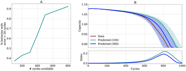
Our model can integrate and predict longer input trajectories without having to retrain. This allows us to flexibly decide how many cycles the cell should go through and predict the remaining capacity trajectory with our model. If a higher accuracy is desired, the battery can be cycled longer, resulting in more information available for prediction and consequently higher accuracy. Importantly, this is a different scenario from the one presented in Fig. 5. In Fig. 5 we show the impact of varying the initial number of cycles with which the model is trained. In contrast, in Fig. 6 we use a fixed model and simply append cycles to show how the accuracy and projected uncertainty of the prediction changes, allowing a flexible trade-off between cycling time, accuracy, and uncertainty.

Fig. 6 More cycle information decreases uncertainty and error. (A) Percentage of batteries with an error of less than 50 cycles for EOL when more input cycles are available. (B) (Upper) Uncertainty and error are reduced when more input cycles are available. Inputting 300 cycles (blue trajectory) reduces the error and uncertainty. (Lower) Standard deviation is plotted for easier quantitative comparison. The blue trajectory is closer to the real trajectory and shows less uncertainty.

In Fig. 6A we show the percentage of batteries for which the prediction for EOL is less than fifty cycles off from the true EOL dependent on the number of cycles used as input for the model. As expected, the proportion of accurate predictions increases as more cycling information becomes available.

Since the uncertainty over the EOL is reduced when the battery is cycled for longer, batteries can be cycled until the desired uncertainty is reached. In Fig. S7 (in the ESI†) we show that uncertainty and accuracy are strongly inversely correlated, implying that the accuracy will increase as more cycles become available. In Fig. S3† we additionally show results for the NMC dataset.

In Fig. 6B we show for one exemplary battery how the predicted uncertainty changes. We see that the uncertainty is reduced and that the prediction becomes more accurate when more cycle information is input.

3.5 Inspecting what the LSTM has learned

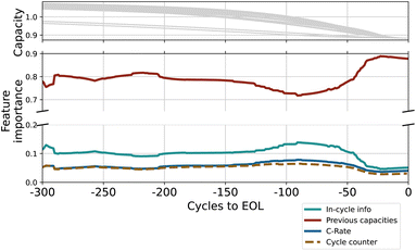
In addition to accurate prediction, we are interested in analyzing which features were important for prediction and whether they reflect prior knowledge about the chemical processes inside the battery cell. We analyze the relative importance of the inputs in the predictions, differences between short- and long-lived batteries as well as calendar-aged and non-aged batteries.

For this analysis, we compute the gradient of the output with respect to the input. The gradient indicates how fast the output changes with a change in the respective input variable, representing an intuitive measure of feature importance. To make the resulting importance measures comparable between cycles and batteries, we normalize them so that the total importance of all input features for one battery cell sums up to one. We show the results of this analysis averaged over the test set in Fig. 7 and 8. The data in Fig. 2 shows that the capacity trajectory of LFP batteries consists of a relatively flat initial regime followed by a phase in which the cell capacity decreases rapidly until the EOL. The point at which the cell enters the rapid decline phase is often visible as a knee point in the trajectory. Since this point is a determining factor of a battery's life, it is of particular interest what triggers this transition. We visualize the gradients over the last 300 cycles (as predicted by an exemplary LSTM for each battery cell).

Fig. 7 Sensitivity to input features over the last 300 cycles. The importance of covariates increases around the knee point. (Upper row) Capacity trajectories (for orientation). (Middle and lower row) Absolute gradients of all input-features.

Fig. 8 Sensitivity to input features over the last 300 cycles. Long- and short-lasting batteries show qualitative difference in the importance of coulombic efficiency. (Upper row) Capacity trajectories (for orientation) (Lower row) Absolute gradients of coulombic efficiency.

In Fig. 7 we show the importance of the input features averaged over the test set along with the capacity trajectories. We observe that the importance of the previous capacity stays relatively constant over the lifetime of the battery until approximately 200 cycles before the EOL. At this point, there is a dip in importance for the capacity trajectory and the covariates gain more relevance. Our interpretation is that the cycling conditions such as the charge and discharge rate are more relevant in predicting the ‘point of descent’, and thus the EOL, whereas the capacity in previous cycles is more relevant for predicting the shape of the capacity trajectory.

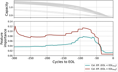
In the phase of quick degradation, we note that the importance of previous capacities increases again, becoming the almost sole determining factor for the output. We hypothesize that once degradation enters an accelerated phase, the only relevant factor for prediction appears to be the current rate of degradation, which is encoded in the previous capacities values. In Fig. 8 we additionally visualize the mean importance of coulombic efficiency over the last 250 cycles, as calculated for long- (red) and short-lasting (green) batteries; since the average lifetime of the dataset is 691 cycles, we use 700 cycles as the cutoff value. There is a qualitative difference in the importance of coulombic efficiency for long- and short-lasting batteries, both in the absolute value but also in the proportional increase of importance as a battery approaches its EOL. For short-lived batteries, the importance increases slightly but steadily as the batteries approach EOL. Low coulombic efficiency is possibly due to high SEI forming exchange current density that leads to loss of active lithium.⁴³ The expedited loss of cyclable lithium leads to rapid capacity loss. Thus, low coulombic efficiency can be an indicator of a shortened cell life. The importance of coulombic efficiency increasing proportionally more for short-lived than long-lived batteries is in line with our understanding of the internal state of the battery.

In Fig. 9 we show the importance of the in-cycle information (overpotential, coulombic efficiency, and variance in the difference between charge and discharge) for the last 250 cycles for calendar-aged and non-calendar-aged batteries. Since calendar-aged batteries have a much higher mean lifetime than non-aged batteries, we consider only non-aged batteries with a lifetime longer than 600 cycles. In this way, both sets of batteries have approximately the same average lifetime. We observe that there is a quantitative difference in the gradients, i.e. the importance of in-cycle information differs for calendar-aged and non-aged batteries from the 250th to last to the 100th to the last cycle. The lifetime of calendar-aged cells is more affected by the cycling conditions. The quantitative difference indicates that the LSTM discriminates already from the initial cycles that calendar-aged and non-aged cells belong to different data distributions. Such difference is also manifested in higher uncertainty for the calendar-aged cells.

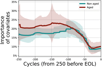Fig. 9 Importance of in-cycle information for calendar-aged and non-calendar-aged batteries. The shaded area indicates one standard deviation in each direction.

4 Conclusions

We have proposed and demonstrated a data-efficient autoregressive model for the early prediction of battery degradation that supports uncertainty awareness (both epistemic and aleatoric), explainability, and chemistry-agnostic modeling while predicting the entire degradation trajectory. It relies on features that are easy to obtain from simple charge/discharge curves during the early cycling. With an explainability analysis, we show differences in the importance of particular input features for long- and short-lived battery cells and connect these differences to known chemical effects during degradation.

A limitation of our work is that the main dataset consists only of cells with a single cell chemistry that are discharged with a uniform discharge rate across cells and lifetime. As opposed to the more realistic use case of varying charge/discharge rates, this limits the complexity of the prediction task. In subsequent work, we intend to apply the model to newly created datasets containing a wider variety of usage parameters, opening up the possibility of incorporating the model into a BMS (Battery Management System) for more targeted usage. Additionally, as is visible in Fig. 4 the model is still slightly overconfident in its predictions, particularly for data points with large errors. In future work, we plan to predict the driving degradation mechanism directly from the LSTM model.

As we model uncertainty directly and the model is chemistry agnostic, such a model can be reliably trained and deployed for existing and new classes of cell chemistries in the future. We show the potential with a preliminary model trained with a small dataset of openly available but limited NCA and NMC cell cycling data.

Early prediction with our uncertainty-aware model will create the basis for an accelerated autonomous battery design platform by shortening the time-consuming life cycle assessment tests. As our model predicts the whole trajectory with uncertainty and is flexible towards the length of initial input cycles, it is well suited for such use cases where the actual length of cycling tests varies. Access to model uncertainty opens up the possibility of building accurate models for new cell chemistries with limited amounts of data collection via active learning.

Data availability

The code for this paper can be found at https://github.com/laura-rieger/battery-life-prediction. This study was carried out using publicly available data from https://github.com/rdbraatz/data-driven-prediction-of-battery-cycle-life-before-capacity-degradation at https://data.matr.io/1/projects/5c48dd2bc625d700019f3204 and https://www.batteryarchive.org/snl_study.html.

Author contributions

A. B. conceptualized and supervised the project; L. R. with input from A. B. and O. W. designed and developed the model and method; E. F. collected, processed and featurized the data; E. F. and L. R did the workflow and result visualizations; L. R. carried out the software engineering, including implementation of model and training framework, implementation of data workflows for the datasets, and analysis of data. All authors participated in the discussion and formal analysis of results; L. R., E. F., A. B. prepared the first draft and all authors contributed to review and editing; T. V. and A. B. did funding acquisition.

Conflicts of interest

There are no conflicts to declare.

Acknowledgements

The authors acknowledge the European Union's Horizon 2020 research and innovation program under grant agreement No 957189 (BIG-MAP) and No 957213 (BATTERY2030PLUS).

Notes and references

1. O. Schmidt, S. Melchior, A. Hawkes and I. Staffell, Joule, 2019, 3, 81–100.
2. T. Le Varlet, O. Schmidt, A. Gambhir, S. Few and I. Staffell, J. Energy Storage, 2020, 28, 101230.
3. M.-F. Ng, J. Zhao, Q. Yan, G. J. Conduit and Z. W. Seh, Nat. Mach. Intell., 2020, 2, 161–170.
4. Y. Li, K. Liu, A. M. Foley, A. Zülke, M. Berecibar, E. Nanini-Maury, J. Van Mierlo and H. E. Hoster, Renewable Sustainable Energy Rev., 2019, 113, 109254.
5. J. Zhang and J. Lee, J. Power Sources, 2011, 196, 6007–6014.
6. J. S. Edge, S. O'Kane, R. Prosser, N. D. Kirkaldy, A. N. Patel, A. Hales, A. Ghosh, W. Ai, J. Chen and J. Yang, et al. , Phys. Chem. Chem. Phys., 2021, 23, 8200–8221.
7. P. M. Attia, A. Grover, N. Jin, K. A. Severson, T. M. Markov, Y.-H. Liao, M. H. Chen, B. Cheong, N. Perkins and Z. Yang, et al. , Nature, 2020, 578, 397–402.
8. X. Liu, W. Ai, M. N. Marlow, Y. Patel and B. Wu, Appl. Energy, 2019, 248, 489–499.
9. J. T. Warner, The handbook of lithium-ion battery pack design: chemistry, components, types and terminology, Elsevier, 2015, pp. 91–101.
10. K. A. Severson, P. M. Attia, N. Jin, N. Perkins, B. Jiang, Z. Yang, M. H. Chen, M. Aykol, P. K. Herring and D. Fraggedakis, Nat. Energy, 2019, 4, 383–391.
11. T. Vegge, J.-M. Tarascon and K. Edström, Adv. Energy Mater., 2021, 11, 2100362.
12. M. Aykol, C. B. Gopal, A. Anapolsky, P. K. Herring, B. v. Vlijmen, M. D. Berliner, M. Z. Bazant, R. D. Braatz, W. C. Chueh and B. D. Storey, J. Electrochem. Soc., 2021, 168, 030525.
13. X. Hu, L. Xu, X. Lin and M. Pecht, Joule, 2020, 4, 310–346.
14. J. Guo, Z. Li and M. Pecht, J. Power Sources, 2015, 281, 173–184.
15. Y. Zhang, R. Xiong, H. He and M. G. Pecht, IEEE Trans. Veh. Technol., 2018, 67, 5695–5705.
16. A. Aitio and D. A. Howey, Joule, 2021, 5, 3204–3220.
17. T. Baumhöfer, M. Brühl, S. Rothgang and D. U. Sauer, J. Power Sources, 2014, 247, 332–338.
18. W. Li, N. Sengupta, P. Dechent, D. Howey, A. Annaswamy and D. U. Sauer, J. Power Sources, 2021, 506, 230024.
19. J. Hong, D. Lee, E.-R. Jeong and Y. Yi, Appl. Energy, 2020, 278, 115646.
20. C. Strange and G. Dos Reis, Energy and AI, 2021, 5, 100097.
21. N. Srivastava, G. Hinton, A. Krizhevsky, I. Sutskever and R. Salakhutdinov, J. Mach. Learn. Res., 2014, 15, 1929–1958.
22. S. Saxena, L. Ward, J. Kubal, W. Lu, S. Babinec and N. Paulson, J. Power Sources, 2022, 542, 231736.
23. B. Jiang, W. E. Gent, F. Mohr, S. Das, M. D. Berliner, M. Forsuelo, H. Zhao, P. M. Attia, A. Grover and P. K. Herring, et al. , Joule, 2021, 5, 3187–3203.
24. N. H. Paulson, J. Kubal, L. Ward, S. Saxena, W. Lu and S. J. Babinec, J. Power Sources, 2022, 527, 231127.
25. A. Bhowmik, M. Berecibar, M. Casas-Cabanas, G. Csanyi, R. Dominko, K. Hermansson, M. R. Palacin, H. S. Stein and T. Vegge, Adv. Energy Mater., 2021, 2102698.
26. J. Amici, P. Asinari, E. Ayerbe, P. Barboux, P. Bayle-Guillemaud, R. J. Behm, M. Berecibar, E. Berg, A. Bhowmik and S. Bodoardo, et al. , Adv. Energy Mater., 2022, 2102785.
27. M. Fichtner, K. Edström, E. Ayerbe, M. Berecibar, A. Bhowmik, I. E. Castelli, S. Clark, R. Dominko, M. Erakca and A. A. Franco, et al. , Adv. Energy Mater., 2021, 2102904.
28. Y. Preger, H. M. Barkholtz, A. Fresquez, D. L. Campbell, B. W. Juba, J. Romàn-Kustas, S. R. Ferreira and B. Chalamala, J. Electrochem. Soc., 2020, 167, 120532.
29. S. Hochreiter and J. Schmidhuber, Neural Comput., 1997, 9, 1735–1780.
30. J. Busk, P. B. Jørgensen, A. Bhowmik, M. N. Schmidt, O. Winther and T. Vegge, Mach. Learn.: Sci. Technol., 2021, 3, 015012.
31. B. Lakshminarayanan, A. Pritzel and C. Blundell, NIPS, 2017.
32. D. P. Kingma and J. Ba, Adam: A Method for Stochastic Optimization, ICLR, 2015.
33. A. Paszke, S. Gross, F. Massa, A. Lerer, J. Bradbury, G. Chanan, T. Killeen, Z. Lin, N. Gimelshein, L. Antiga, et al., Proceedings of the 33rd International Conference on Neural Information Processing Systems, 2019, pp. 8026–8037.
34. S. Sun, T. Guan, P. Zuo, Y. Gao, X. Cheng, C. Du and G. Yin, ChemElectroChem, 2018, 5, 2301–2309.
35. P. Zhang, T. Yuan, Y. Pang, C. Peng, J. Yang, Z.-F. Ma and S. Zheng, J. Electrochem. Soc., 2019, 166, A5489.
36. Y. Abe, N. Hori and S. Kumagai, Energies, 2019, 12, 4507.
37. M. Dubarry, C. Truchot and B. Y. Liaw, J. Power Sources, 2012, 219, 204–216.
38. X. Han, M. Ouyang, L. Lu, J. Li, Y. Zheng and Z. Li, J. Power Sources, 2014, 251, 38–54.
39. I. Bloom, A. N. Jansen, D. P. Abraham, J. Knuth, S. A. Jones, V. S. Battaglia and G. L. Henriksen, J. Power Sources, 2005, 139, 295–303.
40. C. Lv, X. Zhou, L. Zhong, C. Yan, M. Srinivasan, Z. W. Seh, C. Liu, H. Pan, S. Li and Y. Wen, et al. , Adv. Mater., 2022, 34, 2101474.
41. Y. Ma, L. Wu, Y. Guan and Z. Peng, J. Power Sources, 2020, 476, 228581.
42. A. Moretti, V. Sharova, D. V. Carvalho, A. Boulineau, W. Porcher, I. de Meatza and S. Passerini, Batteries Supercaps, 2019, 2, 240–247.
43. P. Dechent, S. Greenbank, F. Hildenbrand, S. Jbabdi, D. U. Sauer and D. A. Howey, Batteries Supercaps, 2021, 4, 1821–1829.

---

Footnote

† Electronic supplementary information (ESI) available. See DOI: https://doi.org/10.1039/d2dd00067a

---