
 Open Access Article
 This Open Access Article is licensed under a
 Creative Commons Attribution 3.0 Unported Licence
Unravelling the effect of paramagnetic Ni2+ on the 13C NMR shift tensor for carbonate in Mg2−xNixAl layered double hydroxides by quantum-chemical computations†
Megha
Mohan
a,
Anders B. A.
Andersen‡
b,
Jiří
Mareš
 a,
Nicholai Daugaard
Jensen
b,
Ulla Gro
Nielsen
*b and
Juha
Vaara
*a
a,
Nicholai Daugaard
Jensen
b,
Ulla Gro
Nielsen
*b and
Juha
Vaara
*a
aNMR Research Unit, P.O. Box 3000, FI-90014 University of Oulu, Finland. E-mail: juha.vaara@oulu.fi
bDepartment of Physics, Chemistry and Pharmacy, University of Southern Denmark, Campusvej 55, DK-5230 Odense, Denmark. E-mail: ugn@sdu.dk
First published on 23rd August 2023
Abstract
Structural disorder and low crystallinity render it challenging to characterise the atomic-level structure of layered double hydroxides (LDH). We report a novel multi-step, first-principles computational workflow for the analysis of paramagnetic solid-state NMR of complex inorganic systems such as LDH, which are commonly used as catalysts and energy storage materials. A series of 13CO32−-labelled Mg2−xNixAl-LDH, x ranging from 0 (Mg2Al-LDH) to 2 (Ni2Al-LDH), features three distinct eigenvalues δ11, δ22 and δ33 of the experimental 13C chemical shift tensor. The δii correlate directly with the concentration of the paramagnetic Ni2+ and span a range of |δ11 − δ33| ≈ 90 ppm at x = 0, increasing to 950 ppm at x = 2. In contrast, the isotropic shift, δiso(13C), only varies by −14 ppm in the series. Detailed insight is obtained by computing (1) the orbital shielding by periodic density-functional theory involving interlayer water, (2) the long-range pseudocontact contribution of the randomly distributed Ni2+ ions in the cation layers (characterised by an ab initio susceptibility tensor) by a lattice sum, and (3) the close-range hyperfine terms using a full first-principles shielding machinery. A pseudohydrogen-terminated two-layer cluster model is used to compute (3), particularly the contact terms. Due to negative spin density contribution at the 13C site arising from the close-by Ni2+ sites, this step is necessary to reach a semiquantitative agreement with experiment. These findings influence future NMR investigations of the formally closed-shell interlayer species within LDH, such as the anions or water. Furthermore, the workflow is applicable to a variety of complex materials.
1. Introduction
Layered double hydroxides (LDH) are a class of layered inorganic ionic solids characterised by the general formula M(II)1−xM(III)x(OH)2Anx/n·yH2O, where M(II) [M(III)] is a divalent [trivalent] cation in the metal hydroxide layers, the layers are separated by an interlayer containing anions (An) with a charge of n− and a variable amount of water.1–3 The M(III) content, x, ranges between 1/6 and 1/3, hence these materials are often referred to as “M(II)M(III)-LDH”. The anions are weakly bound and highly exchangeable, which renders LDH a rare example of anion-exchange materials,4–7 and therefore allows potential use for, e.g., drug delivery8 and environmental remediation.5 Moreover, LDH are used as catalysts9 and energy materials due to the variable oxidation states of transition metals within the cation layers.10Characterisation of LDH by X-ray diffraction (XRD) is challenging due to structural disorder (such as a mixed M(II) and M(III) occupancy), stacking faults, and interstratification of different polytypes leading to structural ambiguity often combined with nanosized particles.11 Powder XRD (PXRD), the preferred characterisation technique, only reports on the average structure instead of the detailed local structure. Solid-state NMR (SSNMR) has advanced our understanding of the atomic-level structure of LDH, especially the local structure of the cation layer and the disordered and dynamic interlayer.12 For example, 1H magic-angle spinning (MAS) NMR using ultrafast rotation has confirmed cation ordering in the metal hydroxide layer (Al–O–Al avoidance)13 and the metal-ion distribution in trimetallic Mg2−xNixAl-LDH.14 SSNMR has also given insight into the highly disordered interlayer, such as revealing a dynamic exchange between carbonate and bicarbonate,15 as well as CO2 exchange with the atmosphere.16
The most detailed crystal structures have been obtained from single-crystal XRD studies of MgAl-LDH minerals with carbonate (CO32−) as anion. These have, for quintinite (Mg4Al2(OH)12CO3·3H2O) – a MgAl-LDH with a Mg![[thin space (1/6-em)]](https://www.rsc.org/images/entities/char_2009.gif) :Al ratio of 2:1, confirmed ordering of the metal ions.17 The crystal structure of such a LDH is illustrated in Fig. 1, involving a “honeycomb” cation layer structure for both known quintinite polymorphs (1M and 2T).17,18 The 1M and 2T polymorphs differ in the stacking of the cation layers. The interlayer has a high degree of structural disorder, which is reflected by the presence of multiple carbonate sites and water sites with partial occupancy for both structures. Recently, a combination of Rietveld refinement of PXRD data and multi-nuclear SSNMR also confirmed a lowering of the space group symmetry to monoclinic for ZnAl-LDH with carbonate in the interlayer.19 Furthermore, both carbonate and bicarbonate (HCO3−) have been identified in the interlayer of diamagnetic MgAl-LDH, where the high Al content (high cation layer charge) favours carbonate.15 These two anions can be distinguished based on a 10 ppm difference in the 13C isotropic chemical shift, δiso(13C), opposite signs of the 13C chemical shift anisotropy and assignment based on a visual comparison with the 13C MAS NMR spectra of sodium carbonate and bicarbonate in MgAl-LDH15 and calcinated MgAl-LDH.20
:Al ratio of 2:1, confirmed ordering of the metal ions.17 The crystal structure of such a LDH is illustrated in Fig. 1, involving a “honeycomb” cation layer structure for both known quintinite polymorphs (1M and 2T).17,18 The 1M and 2T polymorphs differ in the stacking of the cation layers. The interlayer has a high degree of structural disorder, which is reflected by the presence of multiple carbonate sites and water sites with partial occupancy for both structures. Recently, a combination of Rietveld refinement of PXRD data and multi-nuclear SSNMR also confirmed a lowering of the space group symmetry to monoclinic for ZnAl-LDH with carbonate in the interlayer.19 Furthermore, both carbonate and bicarbonate (HCO3−) have been identified in the interlayer of diamagnetic MgAl-LDH, where the high Al content (high cation layer charge) favours carbonate.15 These two anions can be distinguished based on a 10 ppm difference in the 13C isotropic chemical shift, δiso(13C), opposite signs of the 13C chemical shift anisotropy and assignment based on a visual comparison with the 13C MAS NMR spectra of sodium carbonate and bicarbonate in MgAl-LDH15 and calcinated MgAl-LDH.20
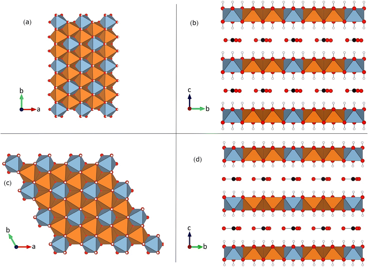 | ||
| Fig. 1 Crystal structure of the Mg2Al-LDH studied in this paper: (a) and (b) 1M and (c) and (d) 2T polytypes illustrating the “honeycomb” superstructure, where all Al (blue) are surrounded by Mg (orange).17,18 View along the LDH layer normal direction in panels (ac) and along one of the in-layer axes in (b) and (d). Representative examples of the interlayer CO32− anions are shown, and the interlayer water molecules have been omitted. In the cation layers, the blue (orange) polyhedra correspond to Al (Mg) sites. | ||
While SSNMR has successfully probed the local structure of diamagnetic LDH,12 the presence of paramagnetic species renders the analysis of SSNMR spectra more challenging. Significant paramagnetic shifts are observed for 27Al in LDH, δiso(27Al), with Co2+, Ni2+ and Cu2+.14,21 While the δiso(27Al) in a series of Mg2−xNixAl(OH)6(CO3)·nH2O, with x ranging from 0 to 2, was shown to scale linearly with the number of Ni2+ ions that neighbour Al in the metal layer (ca. −350 ppm/Ni), the total Ni content (Ni:Al ratio) and interlayer spacing only had a small effect in NiAl-LDH.14 Furthermore, only small paramagnetic shifts (<20 ppm) have been observed for carbonate in NiAl-LDH22 and phosphate MgFe-LDH.23 In these studies, only the isotropic shifts determined from visual inspection of the NMR spectra were reported and no detailed analyses of the NMR spectra have so far been performed. Such analyses can benefit immensely from computational and theoretical methods in the assignment and interpretations of paramagnetic NMR spectra.
Understanding the structure of LDH, including the atomic detail and the effect of paramagnetic doping, is central to link the atomic level structure and materials properties, a pivotal challenge in materials science. This information can now be extracted for diamagnetic systems using SSNMR and first-principles modelling (“NMR crystallography”).24 In contrast, analysis of SSNMR spectra of paramagnetic systems, commonly found in battery, catalytic, and magnetic materials, are challenging. Here we focus on how the concentration of paramagnetic Ni2+ ions in LDH affects the 13C SSNMR spectra of the interlayer carbonate anions. To develop the methodology, we have performed 13C SSNMR measurements of the samples in the solid solutions Mg2−xNixAl(OH)6(CO3)0.5·nH2O, a series of hydrotalcite-type LDH with x = 0, 0.18, 0.34, 0.68, 0.86 and 2. In this series, a specific percentage of diamagnetic Mg2+ ions are replaced by paramagnetic Ni2+ ions carrying two unpaired electrons (S = 1). Such Ni-doped MgAl-LDH are used as precursors for industrial catalysts. A 27Al MAS NMR study of the closely related Mg2−xNixAl(OH)6(NO3)·nH2O series showed cation ordering implying Al–O–Al avoidance, and a random (binomial) distribution of Ni2+ and Mg2+ on the M(II) site.14 The latter reflects the similar ionic radii of Ni2+ (55 pm) and Mg2+ (57 pm). Detailed analyses of the 13C MAS NMR spectra reveals one principal 13C site (see, however, below) with both anisotropy and rhombicity (asymmetry) of the 13C shielding tensor, with the anisotropy scaling linearly with the Ni2+ concentration. In contrast, the isotropic chemical shift, δiso(27Al), only slightly decreases with Ni doping. A recent solid-state 13C MAS NMR study of a Mg1−xNix metal–organic framework material25 found signatures of eight local environments with distinct arrangement of Ni2+ ions in the close vicinity of the 13C centre, and revealed a non-random distribution of nickel metal sites resulting from ferromagnetic and antiferromagnetic couplings between the Ni2+ ions. As noted above, the present Mg2−xNixAl-LDH materials bear no such indications of magnetic couplings. To understand the paramagnetic 13C shifts in the present systems, we compute the pseudocontact shift tensor over a large number of realisations of the random Ni2+ distribution for each of the studied Ni concentrations, by a point-dipole approximation (PDA).26 However, it is found that qualitative agreement with the experimental shielding tensor is only obtained if the local hyperfine contributions resulting from the spin density distribution of the nearby Ni2+ sites, which extends to the interlayer anions, are included in addition to the (expected) local orbital and non-local pseudocontact contributions.
2. Experimental data
Samples
The Mg2−xNixAl-LDH samples (x = 0, 0.18, 0.34, 0.68, 0.83 and 2) were prepared by ion exchange with 13C-labelled carbonate using the corresponding Mg2−xNixAl-LDH with nitrate (NO3−) in the interlayer. The preparation of the parent Mg2−xNixAl-LDH samples has been reported earlier. The parent Mg2Al-LDH with chloride as the interlayer ion was prepared by co-precipitation at constant pH.27 Typically, ca. 200 mg of the LDH was suspended in a solution of ca. 0.40 g sodium bicarbonate in 20 mL of deionised water for 24–48 h, followed by separation by filtering and drying at 60 °C overnight. PXRD confirmed the intercalation of carbonate and preservation of the LDH (see Fig. S1 in the ESI†). While the PXRD diffractograms of polycrystalline (powder) LDH samples show the characteristic features for stacking disorder, i.e., interstratification of different polymorphs, the complexity prevents further analysis. 13C-enriched (99%) sodium carbonate (Na2CO3) and sodium bicarbonate (NaHCO3) were obtained from Sigma-Aldrich and used as received.Solid-state 13C MAS NMR experiments
Solid-state 13C MAS NMR experiments were performed on an Agilent 600 MHz NMR spectrometer (14.1 T) using a 3.2 mm HXY MAS NMR probe tuned to 1H and 13C in double-resonance mode. Adamantane was used as a secondary chemical shift reference, with δ(CH) = 38.3 ppm with respect to TMS (0 ppm). 13C MAS NMR spectra of the paramagnetic (Ni-containing) samples were acquired using a Hahn-Echo sequence (90°-τ-180°-τ-acquisition, τ = 1 rotor period) without 1H decoupling, 10 kHz spinning speed, and with a 90° (180°) pulse of 2.2 (4.4) μs, a relaxation delay of 1 s and 5000–40000 scans. The relaxation time was measured for Mg2−xNixAl-LDH with x = 0.16 to determine the maximum relaxation time needed to ensure quantitative spectra. 13C{1H} CP-MAS spectra were recorded for the diamagnetic Mg2Al-CO3 (7 s relaxation delay, 7000 scans) and NaHCO3 (2 s relaxation delay, 8 scans) using a ramped CP sequence with spinning speeds in the range 3–10 kHz and 5 ms contact time, whereas a single-pulse 13C MAS NMR spectrum was recorded for Na2CO3 (30° pulse, 8 scans, and 900 s relaxation delay). We note that a Hahn-echo sequence or CP was necessary to suppress a large 13C background signal from Kel-F, a fluorinated polymer, in the MAS NMR probe. The magic angle was carefully set by minimising the linewidth of the spinning sidebands from 79Br in KBr. The spectra were processed and analysed using ssNake.28
3. Computational methods
In previous experiments,14 the 27Al NMR chemical shift within the cationic layer of in Mg2−xNixAl-LDH scales linearly with the number of neighbouring, paramagnetic Ni2+ ions. This implies insignificantly small exchange coupling29 between such sites at the measurement temperature, hence the paramagnetic NMR effects caused by the Ni2+ ions on the interlayer anions can be considered additive. The model followed in the present computations of the 13C NMR shielding tensors of the interlayer carbonate anions makes use of this; a flow diagram of the computational procedure is given in Fig. 2. | ||
| Fig. 2 Flow diagram of the chemical shift modelling performed in this work. | ||
In a paramagnetic substance, the NMR shielding tensor is traditionally decomposed as26
| σ = σorb + σcon +σpc, | (1) |
As the NMR spectra of the materials are strongly affected by the paramagnetic Ni2+ dopants randomly introduced on the M(II) sites, we average the pseudocontact shielding σpc over a large number of different random Ni2+ distributions at each Ni concentration. For this, we create a PDA model of an individual Ni2+ site by assigning it a magnetic susceptibility tensor calculated ab initio using correlated wave function theory. We carry out lattice summations of σpc over the Ni2+ distributions using experimental X-ray structures for both 1M and 2T structures (see below), as well as (for comparison) corresponding, computationally optimised structures obtained using a density-functional theory (DFT)/plane-wave pseudopotential method for the diamagnetic Mg2Al-LDH end member of the present LDH series. Finally, a cluster model of the immediate surroundings of the interlayer carbonate is created, in which the anion is sandwiched between the “above” and “below” cationic layers, for calculating the close-range σcon contributions.
Crystal structures
Two high-quality single-crystal X-ray structures of quintinite, Mg4Al2(OH)12(CO3)(H2O)3, from the work of Zhitova et al. have been selected: the 1M structure17 and the 2T structure18 representing the two different polytypes, which differ in their layer stacking. Visualization of the 1M and 2T crystal structures were produced with VESTA (ver. 3.5.8).30 In 1M,17,31 the cation layers are ordered with a rhombohedral stacking sequence, whereas in 2T a hexagonal stacking sequence is found. Both structures contain a highly ordered cation layer with an ideal honeycomb structure where each Al is surrounded by 6 Mg sites (implying Al–O–Al avoidance), as evidenced by the observation of superlattice reflections by XRD. In contrast, the interlayer carbonate anions and water are highly disordered. The 1M structure crystallises in the space group C2/m and the 2T with P![[3 with combining macron]](https://www.rsc.org/images/entities/char_0033_0304.gif) c1, both with a single Al and Mg crystallographic site. The interlayer of the 1M structure contains two crystallographic inequivalent carbon centres (carbonates),18 whereas the 2T structure has 3 crystallographic inequivalent carbons. A large variation is shown in the local hydrogen-bonding environment for carbonate even within the same structure. For example, the two carbon sites of the 1M structure have C2v symmetry and 1 water molecule, all with approximately 1/12 occupancy within the experimental error of the refinement. Similarly, the 2T structure17 features three highly disordered carbonate anions and one water molecule in the interlayer, with occupancy ranging from 0.08 (2T/C2) to 0.14 (C1, C3).
c1, both with a single Al and Mg crystallographic site. The interlayer of the 1M structure contains two crystallographic inequivalent carbon centres (carbonates),18 whereas the 2T structure has 3 crystallographic inequivalent carbons. A large variation is shown in the local hydrogen-bonding environment for carbonate even within the same structure. For example, the two carbon sites of the 1M structure have C2v symmetry and 1 water molecule, all with approximately 1/12 occupancy within the experimental error of the refinement. Similarly, the 2T structure17 features three highly disordered carbonate anions and one water molecule in the interlayer, with occupancy ranging from 0.08 (2T/C2) to 0.14 (C1, C3).
To gain a practical computational model for geometry optimisations and calculating σorb, unit cells were built for the CASTEP code32 from the cif-file obtained from the published single crystal X-ray structures into which explicit carbonate and water molecules were put in place, instead of the partially occupied carbonates and waters to match the chemical formula of Mg4Al2(OH)12(CO3)·3H2O. Thus, three water molecules per carbonate were inserted. Whereas the 1M cell contain two crystallographic inequivalent carbon sites as in the original cif file, the practical realisation of the 2T cell contains four crystallographic inequivalent carbons, i.e., one of the original inequivalent carbon sites of the X-ray structure is in the computations represented by two carbons (the 2T/C1 and 2T/C3 sites). The resulting 1M and 2T unit cells (both atomic positions and unit cell parameters) were then geometry-optimised in CASTEP without symmetry restrictions using the PBE functional33 empirical dispersion correction of the Grimme G06 type,34 Koelling–Harmon treatment of scalar relativistic effects,35 and the large plane-wave cut-off of 630 eV. The supercell contained 86/172 ions for the 1M/2T structures, and the k-space was sampled by a Monkhorst–Pack grid36 with 0.1 Å−1 spacing. The optimised geometries for the 1M and 2T structures are given in the ESI,† Tables S1 and S2. In the geometry optimisations, the Mg2Al-LDH end member (x = 0) was used. Fig. 3 illustrates the optimised structures for 1M and 2T, with the different 13C sites indicated.
 | ||
| Fig. 3 Computationally optimised unit cells of the (a) 1M and (b) 2T simulation cells with the individual 13C sites indicated. | ||
Orbital shielding
CASTEP37,38 was subsequently used to calculate the orbital shielding tensors σorb of the two (1M/C1-2) or four (2T/C1-4) carbon sites in the optimised, diamagnetic Mg2Al-LDH geometry, with water molecules present. Similar computational choices were made as for the geometry optimisation. The numerical precision was checked by carrying out the entire process (including geometry optimisation and the shielding tensor computation) twice, using the increased cut-off of 900 eV and denser k-point sampling (with 0.08 and 0.05 Å−1 spacing of the Monkhorst–Pack grid for 1M and 2T, respectively) on the second time. The two series of calculations showed maximum changes of the order of 1 ppm in the resulting components of σorb, and the better of these two sets of calculations (which we use in the following) can be considered well-converged. As the water molecules were manually added to the positions in between the carbonate ions, an element of non-generality remains in their arrangement and, thus, the hydrogen-bonding situation of the carbonate ions. The resulting local environments are described below. The calculated eigenvalues of orbital shielding tensor σorb were converted to the chemical shift eigenvalues δii (i = 1–3) by subtracting from the isotropic 13C shielding constant of TMS, σC = 179 ppm, obtained using similar methodology in CASTEP.Pseudocontact shielding
Pseudocontact shielding was calculated using a PDA model that assumes that the NMR nucleus is far enough from the centre with unpaired electrons, so that the contact-type and other interactions that depend on the extent of delocalisation of the electron spin no longer influence the shielding (this turned out to be insufficient, vide infra). The paramagnetic metal site is in this model furnished with a susceptibility tensor that can be calculated from the g-tensor and the zero-field splitting (ZFS) tensor of that centre26 as: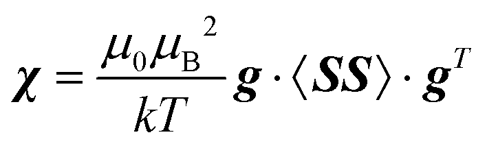 | (2) |
Here, g is the g-tensor, 〈SS〉 is the dyadic of the effective spin operator S,39 and the other symbols have their usual meanings. The pseudocontact shielding at the site of the distant NMR nucleus is calculated from the susceptibility and the relative position of the NMR nucleus with respect to the paramagnetic centre as
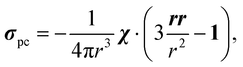 | (3) |
Susceptibility of the Ni2+ site
We constructed finite molecular cluster models cut out from the LDH layers for computing χ for an isolated paramagnetic Ni site. Three different-size cluster models (“small”, “medium” and “large”), each centred at the Ni2+ ion and extending to an increasing number of neighbouring metal sites, were constructed and subjected to pseudohydrogen termination.45 The process was performed similarly as in a recent paper46 and the present details as well as the resulting clusters can be found in the ESI.† The Ni sites have cylindrical symmetry, hence the unique axes of the g-tensor, the ZFS tensor and the resulting χ all coincide with the layer normal direction. With such a cylindrically symmetric susceptibility, the contribution from a single paramagnetic Ni2+ centre to the shielding tensor of a distant NMR nucleus in the PDA becomes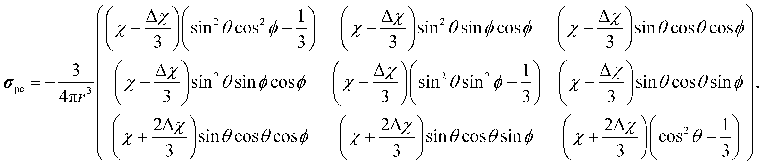 | (4) |
The g- and ZFS tensors were calculated for the optimised structures of the single Ni2+-site models using the ORCA software47 at the state-average complete active space (SA-CASSCF) level using eight electrons in the five orbitals [CAS(8,5)] arising from the 3d shell of the metal ion. The calculations included 10 and 15 states in the triplet and singlet manifolds, respectively. The one-component wave functions were optimised using the scalar relativistic second-order Douglas–Kroll–Hess (DKH2) Hamiltonian48,49 after which the spin–orbit Hamiltonian was diagonalised in the basis of the SA-CASSCF wave functions in a quasi-degenerate perturbation theory process, to calculate the magnetic properties.50,51 In addition, the strongly contracted N-electron valence-state perturbation theory of second order (NEVPT2)52–54 could be applied to the smallest of the three models for the Ni centre, to estimate dynamical correlation effects. The results in Table 1 indicate that the (expected cylindrically symmetric) g- and ZFS tensors, as well as the resulting susceptibility, converge rapidly with the model size. This reflects the localised electron spin density distribution, which houses the spin-density distribution well within its confines (Fig. S3, ESI†). The isotropic g-value at the CASSCF (NEVPT2) level is obtained as 2.27 (2.21), and the corresponding result for the g-tensor anisotropy g‖ − g⊥ is 0.04 (0.03). The D-parameter of the ZFS equals −6.6 (−4.7) cm−1, indicating a moderately easy-axis magnetic nature of the Ni centre. Similar first-principles methodology was recently used for the individual Ni2+ sites in nickelalumite (NiAl4(OH)12SO4·3H2O), an LDH mineral, resulting in very similar data: g = 2.24, g-anisotropy 0.05 and D = −7.8 cm−1, for which very good agreement was observed with experimental values.46 Due to the good convergence with the model size, in the present paper we used χ resulting from the NEVPT2 calculations of the small model, for the calculations of σpc.
| Model | g -Tensor | ZFS | Susceptibility (10−32 m3) | |||||
|---|---|---|---|---|---|---|---|---|
| g ‖ | g ⊥ | g | D/cm−1 | E/D | χ ‖ | χ ⊥ | χ | |
| a The susceptibility anisotropy appearing in eqn (4) is obtained as Δχ = χ‖ − χ⊥. b Results at the NEVPT2 level in parentheses. | ||||||||
| Smallb | 2.301 | 2.258 | 2.272 | −6.561 | 0.0000 | 9.303 | 8.823 | 8.983 |
| (2.229) | (2.197) | (2.208) | (−4.740) | (0.0001) | (8.709) | (8.368) | (8.482) | |
| Medium | 2.301 | 2.259 | 2.273 | −6.429 | 0.0000 | 9.301 | 8.831 | 8.988 |
| Large | 2.300 | 2.260 | 2.273 | −6.286 | 0.0000 | 9.297 | 8.837 | 8.990 |
Lattice summation
σ pc was obtained as a lattice sum of eqn (4) over all paramagnetic Ni2+ sites that resided within a 70 Å cut-off distance from the 13C sites. The cut-off was selected in test calculations in which we found the total σpc to be converged to ca. 1% with the present choice. As the distribution of the Ni doping in the LDH layers is random, one cannot expect to reproduce the experimental data using any a single structure of the paramagnetic defects. Consequently, we averaged σpc over 3000 randomly chosen distributions of the Ni ions onto the M(II) sites. While the σorb were always obtained for the computationally optimised 1M or 2T models including the interlayer water molecules, the lattice sums of σpc were carried out using the M2+ positions from both the original X-ray structures and the computationally optimised CASTEP structures. A temperature of 300 K was used in all the computations.Close-range shielding model
To calculate the σcon term of eqn (1), we constructed a local cluster model of the immediate surroundings of CO32− including, in addition to the ion itself, “small” (in the same nomenclature as used above for in the calculation of χ) clusters of both adjacent cationic layers. The model is depicted in Fig. 4 and the atomic coordinates are given in Table S7 in the ESI.† The atomic positions were adopted from the periodically optimised 1M unit cell from which the clusters representing the cationic layers were cut out and terminated by pseudohydrogens, as discussed above. Since the local structure of the 1M and 2T polymorphs are similar and mainly differ in the stacking of the cation layers, we used the same local model for both 1M and 2T lattices. | ||
| Fig. 4 (a) The cluster model used in the calculation of the close-range hyperfine contributions to the paramagnetic 13C shielding tensor of the interlayer carbonate. The numbering of the paramagnetic sites corresponds to Table 4. (b) The spin density distribution obtained with the paramagnetic Ni located closest to the carbon centre, i.e., position 1 in Table 4. Positive (negative) isosurfaces are shown in red (blue) with the isovalue of 10−5 a.u. | ||
There are eight M(II) sites in the local model, four on each side of the interlayer carbonate, and we occupied each of these eight sites in turn by the paramagnetic Ni2+ centre with the other seven occupied with diamagnetic Mg2+. From each of the single-centre paramagnetic models we calculated the full hyperfine part σhf of the paramagnetic shielding tensor using Kurland–McGarvey theory40 as
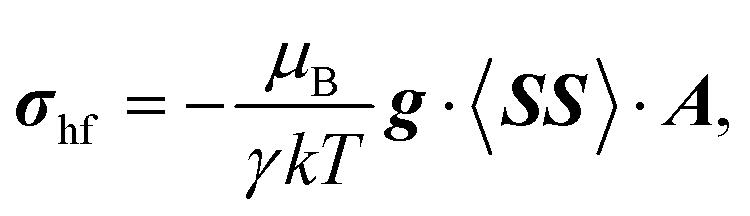 | (5) |
4. Experimental NMR results
The 13C MAS NMR spectra of the six samples are shown in Fig. 5 and the principal components of the shielding tensor determined from analysis of the spinning sideband manifold are reported in Table 2. Given the 33% Al metal fraction in the current study, the carbonate (CO32−) is expected to dominate as the interlayer anion, with only a small amount of bicarbonate (HCO3−).15 This is unambiguously confirmed for diamagnetic Mg2Al-LDH (Table 2). The bicarbonate has both an approx. 5 ppm lower shift and different sign of the Haeberlen chemical shift anisotropy, Δ, than carbonate in the interlayer of both LDH and in sodium (bi)carbonate (Table S8, ESI†). This agrees with a recent study of ZnAl-LDH, which based on Rietveld refinement of PXRD data19 obtained three possible monoclinic structures similar to 1M with one to three crystallographic inequivalent carbon sites, depending on the model and carbonate orientation. However, only a single 13C resonance was observed experimentally for carbonate for the ZnAl-LDH investigated.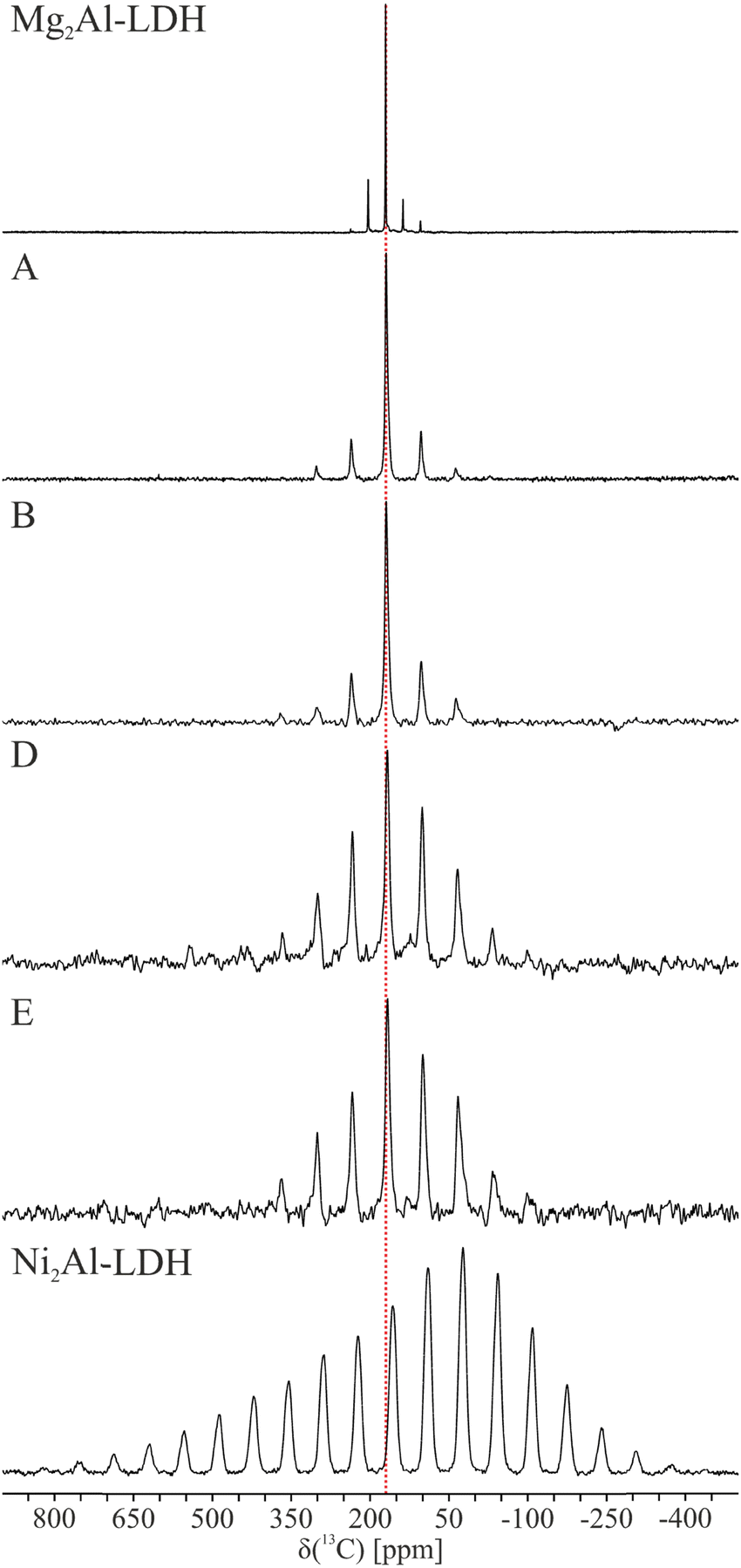 | ||
| Fig. 5 13C MAS NMR spectra of the six the Mg2−xNixAl-LDH samples with x = 0 (Mg2Al-LDH), 0.18 (A), 0.34 (B), 0.66 (D), 0.84 (E), and 2 (Ni2Al-LDH) illustrating increased anisotropy with the Ni content. The red line indicates the isotropic chemical shift for the diamagnetic Mg2Al-LDH. The NMR parameters obtained from the deconvolution of the spectra are reported in Table 2 and simulations using these parameters are shown in Fig. S4 (ESI†). | ||
 with the principal values ordered as δ11 ≥ δ22 ≥δ33. The spectra were recorded at room temperature or slightly above. Errors were estimated visually by varying the parameters and slightly changing the starting guess
| Sample | x | δ 11 | δ 22 | δ 33 | δ |
|---|---|---|---|---|---|
| a It should be noted that δ22 is difficult to precisely determine experimentally, hence the indicated error margins are only indicative. | |||||
| Na2CO3(s) | (Model) | 205(4) | 188(4) | 119(4) | 170.4(3) |
| NaHCO3(s) | (Model) | 227(2) | 145(3) | 121(3) | 164.3(4) |
| Mg2Al-LDH | 0 | 200(4) | 194(10) | 117(3) | 170.3(3) |
| A | 0.18 | 264–267 | 161–148 | 94–81 | 170(2) |
| B | 0.33 | 283–278 | 162–150 | 75–69 | 169(2) |
| D | 0.68 | 342–339 | 159–145 | 3–1 | 167(4) |
| E | 0.84 | 417–416 | 154–129 | −45–−46 | 166(4) |
| Ni2Al-LDH | 2 | 637–636 | 51–48 | −215–−216 | 156(4) |
Visual inspection of 13C MAS NMR spectra shows that only small changes are observed for the isotropic shift, as the difference between the Mg2Al-LDH and Ni2Al-LDH end members is 14 ppm. In contrast, the anisotropy seen, e.g., in the number of spinning sidebands and the linewidth, to increase dramatically with the Ni2+ content. Simultaneously, a change is seen in the sign of the shielding anisotropy for sample A (x = 0.16). The elements of the chemical shift tensor were determined by fitting of the experimental spectra using a single site (See Fig. S4, ESI† and Table 2). This approach reproduced the spectra well at low Ni2+ contents, whereas some deviations are seen at high Ni contents especially for x = 0.84 and 2. This most likely reflects a distribution of the shielding parameters due to the presence of multiples sites in the different LDH polymorphs. Attempts to model the spectra with multiple sites proved ambiguous (six variables added per additional site). This effect is expected to be enhanced with the Ni content. For the low concentrations (x = 0.18 and 0.34), we observe a second site ca. 3 ppm lower, accounting for ca. 20–30% of the total intensity. However, this site is not observed for the diamagnetic Mg2Al-LDH.
Assuming that the Ni2+ sites remain effectively magnetically uncoupled at the measurement temperature, as suggested by the 27Al NMR shift data of the parent Mg2−xNixAl-LDH scaling linearly with the dopant concentration14 (vide supra) one would expect a similar, linear dependence of also the experimental isotropic 13C chemical shifts and shift eigenvalues of the interlayer carbonate anions on x. Taking into account the substantial size of the error margins in the data, this is roughly also observed.
While the conventional Rm crystal structure dictates axial symmetry of the 13C shielding tensor, a significant asymmetry is observed, cf., Table 2, which points to a lowering of the local symmetry in line with the detailed low-symmetry single-crystal X-ray structures (1M and 2T).17,18 We note that the value of δ22 seems to be less precise especially for low Ni content (due to the spectra possessing few spinning side bands in this case) than the other two (δ11 and δ33), which define the edges of the spectrum.
5. Computational results
Local environments and orbital shielding tensors
The local environments for all CO32− resulting from the geometry-optimised 1M and 2T structures are illustrated in Fig. 6. σorb from the CASTEP calculations on the corresponding unit cells are given in Table S9 in the ESI.† A general feature of the optimised geometry is that the carbonate ions invariably seek themselves to the positions in which their oxygen ions are located directly between the M(II)2Al–OH groups of the LDH layers both above and below. Thus, in addition to the in-plane hydrogen bonding with the water molecules, each oxygen “coordinates” both upwards and downwards to the OH groups of the adjacent LDH layers, with the distance of the carbonyl oxygen and the OH-group hydrogen in the range 1.78⋯1.87 Å. A second characteristic feature of the optimised geometry is that the carbonate ions remain parallel with the LDH layers.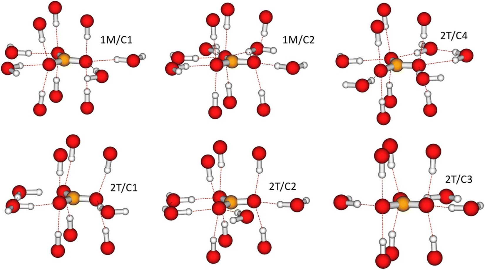 | ||
| Fig. 6 The local hydrogen bonding network for the different CO32− ions to the interlayer water molecules and hydroxyl groups in the cation layer in Mg2Al-LDH using optimised structures. This is shown for the two crystallographic inequivalent carbon sites in the optimized 1M crystal structure (1M/C1 and 1M/C2) and the four carbon sites of the optimized 2T crystal structure. The 2T/C1 and 2T/C3 sites of the computations are two different instantaneous realisations (due to the different hydrogen-bonding pattern) of the same crystallographic position in the 2T structure. | ||
Within the interlayer space, the oxygen atoms of the CO32− ions are hydrogen-bonded to the hydrogen atoms of the water molecules in various patterns. In the 1M structure, two of the three oxygens for carbonates 1M/C1 and 1M/C2 are singly hydrogen-bonded to neighbouring water molecules, whereas the third oxygen of the 1M/C1 (1M/C2) carbonate is coordinated to two (three) waters. In the 2T structure, the carbonate sites 2T/C1 and 2T/C3 are singly hydrogen-bonded via two of their oxygen atoms, whereas the third oxygen is not hydrogen-bonded. The carbonate site 2T/C2 is singly hydrogen-bonded through two of its oxygens and twice bonded through a third oxygen. Hence, the bonding pattern is similar to that of the carbonate site C1 in the 1M structure. Finally, the carbonate site C4 of the 2T structure is doubly hydrogen-bonded to neighbouring waters via two of its oxygen atoms and singly hydrogen-bonded via the third atom. Hence, the altogether six carbon sites of the two structures represent four different hydrogen-bonding patterns, as detailed in Table 3.
| Carbonate sites | 1M/C1 | 1M/C2 | 2T/C1a | 2T/C3a | 2T/C2 | 2T/C4 |
|---|---|---|---|---|---|---|
| a The 2T/C1 and 2T/C3 sites correspond to the same crystallographic site and are only distinguished in the computations due to the different instantaneous hydrogen-bonding situation with the interlayer water molecules in the computationally optimised structure. b The orbital shielding tensor eigenvalue corresponding to the direction along the LDH layer normal. c The orbital shielding tensor eigenvalues corresponding to the direction along the LDH layers. The eigenvalues are ordered such that σ11 > σ22 > σ33. | ||||||
| σ | −2.0 | 2.0 | −2.6 | −1.9 | 0.1 | −2.0 |
| σ 11 | 48.3 | 46.5 | 50.8 | 51.4 | 50.2 | 49.9 |
| σ 22 | −15.7 | 3.4 | −21.3 | −21.9 | −8.5 | −17.1 |
| σ 33 | −38.5 | −44.0 | −37.5 | −35.2 | −41.3 | −38.9 |
| Hydrogen bonding | 2 × single bonded, 1 × double bonded | 2 × single bonded, 1 × triple bonded | 2 × single bonded, 1 × no bond | 2 × single bonded, 1 × no bond | 2 × single bonded, 1 × double bonded | 1 × single bonded, 2 × double bonded |
In the σorb of all the carbon sites in both the 1M and 2T structures, the most shielded eigenvalue (σ33 = 47⋯48 ppm for 1M, 50⋯51 ppm for 2T) always points to the layer normal direction. The isotropic shielding constants are in all cases close to zero, due to the cancellation between the positive σ33 and negative (all σ11 and most σ22 eigenvalues, apart from the 1M/C2 site) eigenvalues. Three first hydrogen-bonding types in Table 3 form a systematic series where two of the oxygen atoms are always singly hydrogen bonded in the interlayer space, whereas the third oxygen atom evolves between non-bonded, double- and triple-bonded configurations. This development is reflected in σorb: while the isotropic shielding constant becomes only slightly more positive, the shielding anisotropy Δσ (with respect to the layer normal direction) goes through a clear decrease from 80 to 67 ppm and the asymmetry parameter, η, increases from 0.3 to 1 in the series. The fourth hydrogen-bonding situation breaks the pattern by featuring only one single-bonded and two double-bonded oxygens, and the resulting σorb again resembles the situation of the first case of Table 3. Hence, the hydrogen-bonding situation and the local environment of CO32− are seen to be reflected primarily in the anisotropic properties of σorb. The experimental spectra reflect an average of the different carbon sites with their hydrogen-bonding patterns, as the water molecules are dynamic on the NMR time scale at room temperature. Hence, the different sites in our model are best viewed as representing a selection of different instantaneous carbonate configurations and, thereby, the variation in NMR parameters.
Local hyperfine contributions
Table 4 lists the results for the isotropic 13C hyperfine shielding constant σcon from the local environment model depicted in Fig. 4. The corresponding data for the full shielding tensors is included in Table S10 (ESI†). In both Table 4 and Table S10 (ESI†), σhf denotes the result of the full quantum-chemical calculation using eqn (5), σ(1)pc is from PDA used for the Ni2+ centre, and σcon = σhf − σ(1)pc is the double counting-eliminated total local hyperfine contribution to be added to the lattice summation results. The sites 1–8 are numbered according to an increasing distance from the 13C site of the interlayer carbonate ion. Fig. 4(b) shows the spin density distribution of the closest site number 1, at the C–Ni distance of 3.7 Å. It is seen that the negative lobe of the spin density extends all the way from the Ni2+ site to the 13C centre, inducing a positive local contribution of σhf = 17.1 ppm to the isotropic shielding constant from this site, arising primarily from the contact hyperfine mechanism. When the shielding constant arising from PDA applied on this Ni2+ centre, σ(1)pc = −3.4 ppm, is subtracted from the result of the full quantum theory computation (eqn (5)), the local contribution that is not captured in the lattice summation process described below, amounts to σcon = +20.5 ppm, for occupied site number one. The fact that the local contact density contribution is arising from negative spin density instead of the direct, positive contribution of the unpaired electrons, underlines the necessity of capturing the electron spin polarisation. Hence, an unrestricted computational method, such as the presently used unrestricted Kohn–Sham DFT procedure, is necessary.| Ni2+ site number | r(Ni–C)/Å | Contribution | Hyperfine terma | |||||||
|---|---|---|---|---|---|---|---|---|---|---|
| Contact (1 + 3) | Dipolar (2) | Orbital (4) | Contact + g-shift (6) | Dipolar + g-shift (7) | Contact + anis. g-shift (8) | Dipolar + anis. g-shift (9) | Total | |||
| a The numbering corresponds to the break-down of the hyperfine terms into physical contributions presented in ref. 39. | ||||||||||
| 1 | 3.70 | σ hf | 17.12 | −0.72 | −0.05 | 1.76 | −0.07 | 0.00 | −1.01 | 17.03 |
| σ (1)pc | −1.11 | −0.88 | 0.00 | −0.11 | −0.09 | 0.00 | −1.23 | −3.43 | ||
| σ con | 18.23 | 0.16 | −0.05 | 1.87 | 0.02 | 0.00 | 0.23 | 20.45 | ||
| 2 | 4.04 | σ hf | 9.31 | −0.47 | −0.03 | 0.96 | −0.05 | 0.00 | −0.66 | 9.06 |
| σ (1)pc | −0.70 | −0.56 | 0.00 | −0.07 | −0.06 | 0.00 | −0.78 | −2.17 | ||
| σ con | 10.02 | 0.09 | −0.03 | 1.03 | 0.01 | 0.00 | 0.12 | 11.23 | ||
| 3 | 4.13 | σ hf | 7.13 | −0.38 | −0.03 | 0.73 | −0.04 | 0.00 | −0.54 | 6.87 |
| σ (1)pc | −0.58 | −0.46 | 0.00 | −0.06 | −0.05 | 0.00 | −0.64 | −1.79 | ||
| σ con | 7.71 | 0.08 | −0.03 | 0.79 | 0.01 | 0.00 | 0.10 | 8.66 | ||
| 4 | 4.67 | σ hf | 3.25 | −0.17 | −0.01 | 0.33 | −0.02 | 0.00 | −0.24 | 3.13 |
| σ (1)pc | −0.25 | −0.20 | 0.00 | −0.03 | −0.02 | 0.00 | −0.27 | −0.76 | ||
| σ con | 3.49 | 0.02 | −0.01 | 0.36 | 0.00 | 0.00 | 0.03 | 3.89 | ||
| 5 | 4.81 | σ hf | 3.98 | −0.16 | −0.01 | 0.41 | −0.02 | 0.00 | −0.22 | 3.98 |
| σ (1)pc | −0.22 | −0.18 | 0.00 | −0.02 | −0.02 | 0.00 | −0.25 | −0.68 | ||
| σ con | 4.20 | 0.02 | −0.01 | 0.43 | 0.00 | 0.00 | 0.02 | 4.66 | ||
| 6 | 4.92 | σ hf | 3.21 | −0.12 | −0.01 | 0.33 | −0.01 | 0.00 | −0.17 | 3.23 |
| σ (1)pc | −0.17 | −0.13 | 0.00 | −0.02 | −0.01 | 0.00 | −0.19 | −0.52 | ||
| σ con | 3.38 | 0.01 | −0.01 | 0.35 | 0.00 | 0.00 | 0.02 | 3.75 | ||
| 7 | 5.10 | σ hf | 0.65 | −0.11 | −0.01 | 0.07 | −0.01 | 0.00 | −0.16 | 0.43 |
| σ (1)pc | −0.14 | −0.10 | −0.01 | 0.41 | −0.01 | 0.00 | −0.14 | 0.01 | ||
| σ con | 0.79 | −0.01 | 0.00 | −0.34 | 0.00 | 0.00 | −0.02 | 0.42 | ||
| 8 | 5.74 | σ hf | 0.40 | −0.03 | 0.00 | 0.04 | 0.00 | 0.00 | −0.04 | 0.37 |
| σ (1)pc | −0.04 | −0.03 | 0.00 | 0.00 | 0.00 | 0.00 | −0.04 | −0.12 | ||
| σ con | 0.44 | 0.00 | 0.00 | 0.05 | 0.00 | 0.00 | 0.01 | 0.49 | ||
| Sum of 1⋯8 | σ hf | 45.0 | −2.2 | −0.2 | 4.6 | −0.2 | 0.0 | −3.0 | 44.1 | |
| σ (1)pc | −3.2 | −2.5 | 0.0 | 0.1 | −0.3 | 0.0 | −3.5 | −9.5 | ||
| σ con | 48.3 | 0.4 | −0.1 | 4.5 | 0.0 | 0.0 | 0.5 | 53.6 | ||
The contributions of the sites 1–8 indicate a rapid reduction for the magnitude of the local hyperfine contributions with distance to the paramagnetic site. For example, the shielding constant is lowered to 0.5 ppm for site 8 located 5.74 Å from the carbon in the local model. For this site, after removal of the corresponding PDA contributions, the local contribution σcon to be added to the lattice-summed σpc is +0.5 ppm, and we deduce that our model is sufficiently large to capture the essential local contributions. The sum of the sites 1–8 amounts to a total contribution of σhf = 44.1 ppm from the local model, converting to σcon = +53.6 ppm when the PDA value is removed. Correspondingly, from the full tensors in Table S10 (ESI†) it is found that the total contribution of local paramagnetic sites 1⋯8 to the shielding anisotropy with respect to the LDH layer normal direction,  , equals no less than −1014 ppm. However, when the corresponding PDA value of Δσ(1)pc = −1119 ppm is subtracted, Δσcon = 105 ppm is left to be added as a local correction to the lattice summation of the PDA contributions. From all this, it is apparent that the spilling of negative spin density to the interlayer space and the consequent σcon contributions to the 13C shielding tensor of CO32− are unexpectedly large and should be included in any meaningful interpretation of the NMR of the intralayer species in such LDH materials. Moreover, this renders the interpretation of experimental T1 relaxation data more complex, as the dipole approximation is violated.56 One should note that the total numbers given above apply directly to 100% Ni2+ substitution to the M(II) sites of the cation layer and, in general the contributions scale linearly with the fractional Ni2+ concentration.
Total isotropic 13C chemical shift
At this point we add the results of the lattice-summed δpc contributions, eqn (3). Fig. 7 compares the total calculated and experimental, isotropic 13C chemical shifts for the different layer stacking models (1M and 2T) and different (X-ray based and geometry optimised) structures. Table 5 gives the associated numerical data. The results are given both excluding the local hyperfine correction, as δorb + δpc, and including the local hyperfine correction, as δorb + δpc + δcon. The computations assume that the paramagnetic Ni2+ ions are magnetically uncoupled. Therefore, a strictly linear dependence of the computed shift observables on x is expected and also obtained from the calculations. The computational isotropic δiso values start from ca. 10 ppm higher values than the experiment for the diamagnetic Mg2Al-LDH parent compound. Errors of this magnitude may be expected from the DFT methodology used for the present calculations of σorb. A comparison, however, of the calculations of an isolated CO32− molecule with the presently employed PBE, a pure DFT functional, and the hybrid PBE0 functional (on the ORCA software) suggests that the use of PBE in the CASTEP calculation of σorb is not a major cause of the 10 ppm deviation from the experiment: the σorb obtained with the two functionals are within 1 ppm of each other. The shift computed as δorb + δpc (the dotted lines in Fig. 7) increases linearly by 8 ppm in the compositional range x = 0–2, regardless of the underlying structure (1M or 2T), or whether the X-ray structure or computationally optimised geometries are used. Even after considering the estimated error margins, an increasing computational δiso is found, which contrasts the decreasing experimental trend as a function of x. As a result of the opposing trends, the deviation of the calculation from the experiment reaches up to ca. 30 ppm by reaching 100% substitution by Ni. As noted above, the experimental data is roughly linear as a function of x, at least considering the error margins, up to the concentration of x = 0.84. However, at 2 the experimental δiso falls below the linear trend.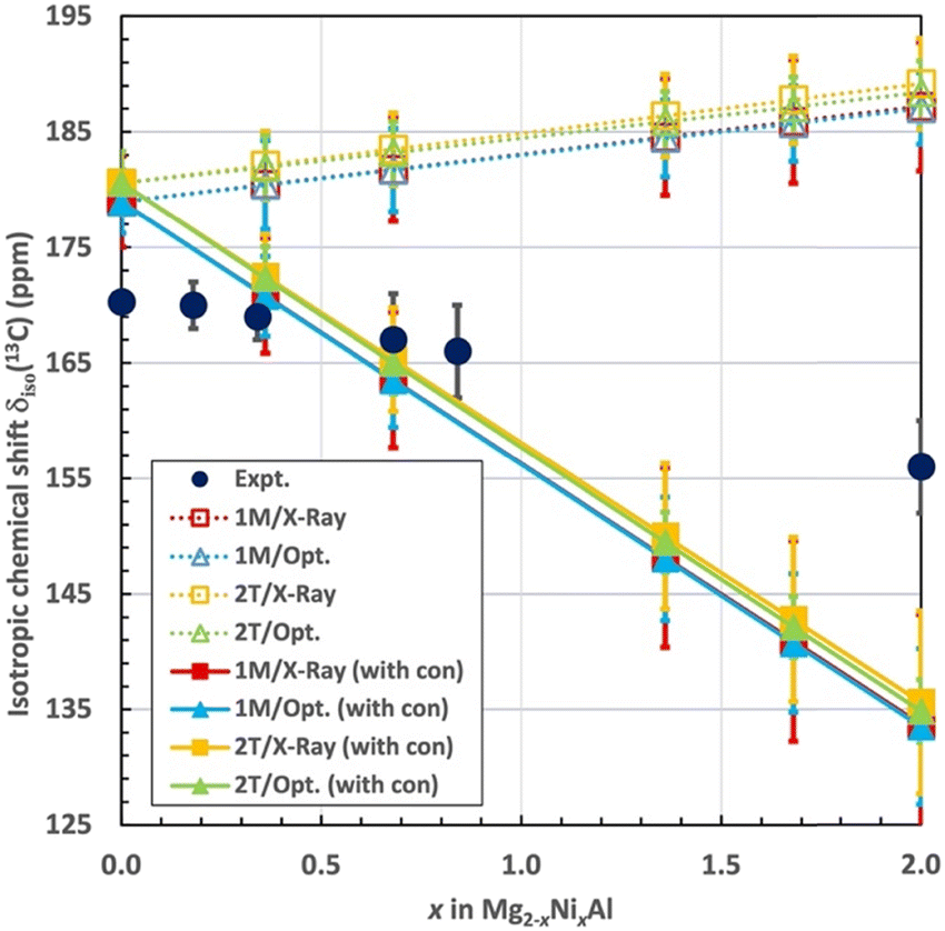 | ||
| Fig. 7 Experimental and calculated isotropic chemical shift δiso(13C) for CO32− in Mg2−xNixAl-LDH as functions of x. The computational results are shown with (solid lines) and without (dotted lines) the local hyperfine contribution σcon. | ||
| Method | Structure | x = 0 | x = 0.36 | x = 0.68 | x = 1.36 | x = 1.68 | x = 2 |
|---|---|---|---|---|---|---|---|
| δ orb + δpc | 1M/X-Ray | 179(4) | 180(4) | 182(5) | 185(5) | 186(5) | 187(6) |
| 1M/Opt. | 179(4) | 180(4) | 182(4) | 184(3) | 186(3) | 187(3) | |
| 2T/X-ray | 181(3) | 182(3) | 184(3) | 186(4) | 188(4) | 189(4) | |
| 2T/Opt. | 181(3) | 182(3) | 183(3) | 186(3) | 187(3) | 188(3) | |
| δ orb + δpc + δcon | 1M/X-Ray | 179(4) | 171(5) | 164(5) | 148(6) | 141(7) | 134(8) |
| 1M/Opt. | 179(4) | 171(4) | 163(4) | 148(5) | 141(5) | 133(5) | |
| 2T/X-Ray | 181(3) | 172(3) | 165(4) | 150(5) | 143(5) | 136(6) | |
| 2T/Opt. | 181(3) | 172(3) | 165(3) | 149(4) | 142(4) | 135(5) | |
Incorporation of the σcon contributions (the solid lines in Fig. 7) flips the trend of the computational results: now the isotropic δiso decreases with x, in qualitative agreement with the experiment. As also the δcon term is simply proportional to x, the computed result at the diamagnetic limit remains roughly 10 ppm overestimated. While the error margins of the computational and experimental data overlap in the region of the intermediate x, at higher Ni2+ concentration, a significantly smaller shift is obtained than observed experimentally. The total computed change of the chemical shift from 0% to 100% Ni amounts to about −45 ppm, clearly overestimating the experimental value of −14.3 ppm. A possible reason for this error could be in the distance between the cation layers, 7.56 Å in the optimised 1M geometry, from which the local hyperfine model was calculated, to be compared with 7.63 and 7.56 Å in the experimental X-ray geometries of 1M and 2T, respectively. We tested the influence of the interlayer distance on the size of δcon by calculations of the model with the closest paramagnetic site, number 1. In this test the interlayer distance was, in turn, extended and diminished by the difference of Δ = 0.06 Å between the experimental and optimised 1M geometries. The results are δcon(site 1) = −21.6, −20.5 and −19.5 ppm for the models with diminished, “standard” and extended interlayer distance. This indicates that the δcon contribution, which is dominated by the contact mechanism, decreases with increasing layer separation, as expected. The overall magnitude of the change amounts to 10% within the investigated distance range, implying that this structural parameter is important for the magnitude of the spin delocalisation to the interlayer species. The obtained change is, nevertheless, too small to cause the overestimation of the decreasing trend of δiso with x in the present computations.
Total anisotropic 13C chemical shift
The results for the anisotropic properties of the shielding tensors can be presented and compared to experiment in three distinct ways:(1) Computed eigenvalues of the total δ (including the δorb, δpc and δcon contributions) are averaged over the 3000 generated Ni2+ distributions for, on the one hand, the two carbon sites of the 1M structure and, on the other hand, the four carbon sites of the 2T structure.
(2) Computed eigenvalues of the two carbon sites of the 1M structure and four carbon sites of the 2T structure are averaged over the Ni2+ distributions and presented individually site-by-site.
(3) Computed, full shielding tensors are averaged over the Ni2+ distributions between, on the one hand, the two sites of the 1M structure and, on the other hand, the four sites of the 2T structure, and the averaged tensors are then subsequently diagonalised to get the eigenvalues.
Methods 1 and 2 involve diagonalisation of the shielding tensor before averaging over sites and both 1M and 2T structures (in 1 and 2). In method 3, averaging of the tensors precedes diagonalisation. The distinction between the two distinct orders of averaging and diagonalisation has been discussed in ref. 57. Methods 1 and 2 are better suited for SSNMR studies on powder (polycrystalline) samples, where the principal values of the shift tensor are the primary observables. The difference between methods 1 and 2 is that the results are presented individually for all the 13C sites in the latter. On the other hand, method 3 corresponds naturally to experiments on single-crystal samples. We choose to focus on method 1 in the following. The results of methods 2 and 3 are briefly discussed in the ESI.† In all cases, the shielding eigenvalues have been converted to chemical shifts.
Fig. 8 illustrates the averaged shift eigenvalues for the two sites of the 1M and for the four sites of the 2T structure. The numerical data are listed in Table 6. The computational shift eigenvalues are linear functions of x (positive slope for δ11, negative for δ22 and δ33). The experimental eigenvalues show a more complicated behaviour, albeit with similar trends when taking visually into account the error margins. The computational eigenvalues cross each other between zero Ni concentration and x = 0.36, which qualitatively matches the experimental observation (vide supra) of the different sign of the shielding anisotropy for sample A with x = 0.18, as compared to the samples with more Ni2+. From that point onwards, the largest calculated shift eigenvalue, δ11, always corresponds to the direction perpendicular to the LDH layers. The computations and experiments agree relatively well, taking into account the error margins of the computations (obtained as mentioned in Fig. 8).
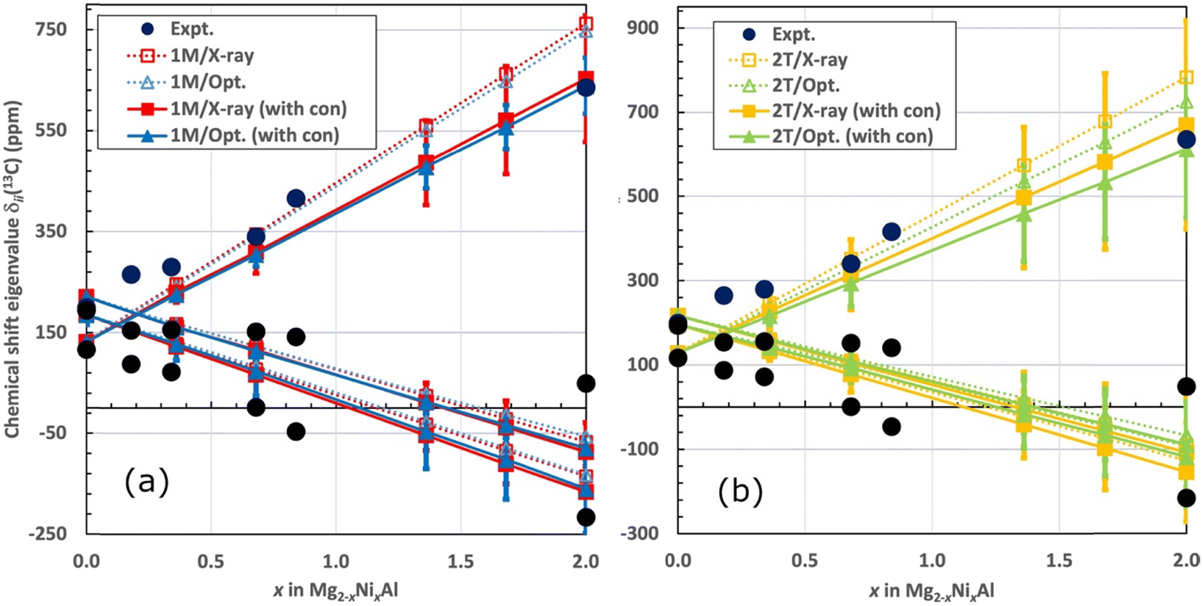 | ||
| Fig. 8 The experimental and computed total 13C chemical shift tensor eigenvalues (top to bottom: δ11, δ22, and δ33, in ppm) for CO32− in Mg2−xNixAl-LDH as functions of x. (a) 1M and (b) 2T structure. The computational results are shown both for the sum of orbital and pseudocontact contributions (dashed lines and open symbols) and added with local hyperfine contribution σcon (full lines and symbols). Averaged eigenvalues are shown following method 1 described in the text. The error margins are placed on the full results (with σcon) based on the maximum difference between the corresponding eigenvalues from the different carbon sites (C1-2 for the 1M structure, C1-4 for 2T). | ||
| Structure | Eigenvalue | x = 0 | x = 0.36 | x = 0.68 | x = 1.36 | x = 1.68 | x = 2 |
|---|---|---|---|---|---|---|---|
| 1M/X-ray | δ 11 | 132(2) | 230(21) | 310(43) | 487(84) | 571(107) | 653(125) |
| δ 22 | 220(6) | 160(15) | 115(24) | 11(38) | −38(52) | −86(58) | |
| δ 33 | 185(19) | 122(7) | 66(5) | −53(31) | −111(39) | −166(51) | |
| 1M/Opt. | δ 11 | 132(2) | 225(7) | 304(23) | 478(43) | 558(43) | 639(56) |
| δ 22 | 220(6) | 161(14) | 113(15) | 12(21) | −33(25) | −79(24) | |
| δ 33 | 185(19) | 127(33) | 73(50) | −46(74) | −102(78) | −159(89) | |
| 2T/X-ray | δ 11 | 128(1) | 227(40) | 314(83) | 497(167) | 583(208) | 669(248) |
| δ 22 | 218(4) | 157(25) | 104(46) | −6(88) | −56(112) | −108(130) | |
| δ 33 | 196(13) | 133(22) | 78(42) | −41(79) | −98(99) | −154(118) | |
| 2T/Opt. | δ 11 | 128(1) | 216(26) | 294(55) | 459(115) | 534(136) | 613(164) |
| δ 22 | 218(4) | 160(12) | 109(33) | 6(67) | −41(85) | −89(102) | |
| δ 33 | 196(13) | 141(19) | 93(34) | −17(80) | −67(97) | −118(119) | |
As functions of x, the computations with only the δorb and δpc contributions (dashed lines and open symbols in Fig. 8) produce systematically too large slope of the shift eigenvalue for the direction perpendicular to the LDH layers (δ11). Incorporation of the local hyperfine contribution δcon (full lines and symbols) significantly improves the overall agreement of the computed δ11 with the experimental data. For the full concentration (x = 2), the values of δ11 without and with the local hyperfine correction are 749 and 639 ppm, respectively, for the optimised geometry of the 1M structure. For the optimised 2T structure, the corresponding results are 726 and 613 ppm, to be compared with the experimental 636–637 ppm (Table 2). These numbers indicate that the effect of δcon is substantial. As in the case of isotropic δiso (vide supra), inclusion of the local hyperfine effect improves the agreement with experiment for the shift eigenvalue δ11 corresponding to the direction of the LDH layer normal. This effect results from the delocalisation of spin density into the carbon site of the interlayer anions and leads to semiquantitative agreement with experiment for this chemical shift eigenvalue.
The shift eigenvalues located in the plane of the LDH layers (δ22 and δ33) become more negative as functions of increasing x. The effect of the local hyperfine contribution is, similarly to that on δ11, to render the calculated δ22 and δ33 more negative than what is obtained with calculations involving the δorb and δpc contributions only (Fig. 8). The effect of δcon is, however, smaller for the in-plane eigenvalues than for δ11: for the full Ni concentration the changes only amount to −30⋯−20 ppm, depending on the structure. The agreement of the calculations with the full range of the experimental δ33 is very satisfactory. In contrast, for the middle eigenvalue, δ22, all the calculated results, including the x = 2 end member of the series, are significantly more negative than the experimental numbers. This results also in the difference between the two computed in-plane eigenvalues to be systematically too small in comparison with experiment, i.e., the shift asymmetry is underestimated by the present calculations. While the situation probably also reflects the fact that the middle eigenvalue is the most difficult to extract precisely from the experimental data, the underestimation of δ22 by the computations is paralleled by the exaggerated decreasing trend of the isotropic shift as a function of x, as discussed above. A possible cause of the lack of quantitative agreement with experiment in the present modelling, for the complete set of shielding observables, is the omission of molecular dynamics effects, primarily among the interlayer species.
Marginally improved agreement with experiment is obtained by using optimised structures as compared to the X-ray structures, as indicated by the triangle symbols (blue and green colour) in Fig. 8 being overall slightly closer to the experimental data points than the squares (red and yellow). The computational results for 13C NMR shift eigenvalues in the 1M and 2T structural models are qualitatively similar. This matches the experimental observation one predominant 13C resonance.
6. Conclusions
Detailed insight into the influence of paramagnetic Ni2+ ion on the 13C NMR parameters was obtained for carbonate intercalated in a series of Mg2−xNixAl-LDH at various values of x from a combined experimental and computational study. Only small changes were observed for the isotropic chemical shifts (ca. 14 ppm for the Ni2Al-LDH end member), which is readily determined experimentally and most often the only parameter reported. In contrast, a clear linear relationship with the Ni2+ content was observed for the tensor eigenvalues determined from detailed analysis of MAS NMR spectra. We devised a computational workflow in which quantum-chemical calculations were carried out including the orbital chemical shift combined with long-distance pseudocontact shifts obtained from a lattice sum averaged over randomly distributed paramagnetic sites, for which the magnetic susceptibility was computed ab initio, as well as the local hyperfine contribution to which the contact term makes a significant contribution.A total of six different carbonate configurations stem from the models created for the 2T and 1M polymorphs, which provided detailed insight into how variations in the local hydrogen-bonding network affects the NMR shift parameters as a function of Ni2+ content. Experimentally, a single site dominated, which contains the average of these different positions. In the computations, only small variations (>2 ppm) were observed for the isotropic shifts arising from the orbital mechanism, whereas changes up to 10 ppm were obtained for the orbital shift eigenvalues. Larger effects up to hundreds of ppm in the eigenvalues were found from the paramagnetic hyperfine shift, where three computational methods differing in the order of the matrix diagonalisation and averaging over the Ni dopant distribution and the individual carbon sites in these parent structures were applied in extracting the shift eigenvalue data. All the methods resulted by design in a linear dependence of the shielding eigenvalues on Ni2+ dopant concentration. It was mandatory to include local hyperfine effects resulting from delocalisation of the Ni2+ spin density, in addition to the expected orbital and pseudocontact contributions, to achieve good agreement with experiment for two of the three shift tensor eigenvalues. In contrast, the choice of using either experimental X-ray or computationally optimised crystal structures was found to be somewhat less crucial.
A qualitative agreement of theory with experiment was achieved in this, original computation of the NMR shielding tensor of the paramagnetic, Ni-doped solid solutions of LDH materials. While the results are not perfect, trends have been reproduced and valuable experience in the modelling of such complex inorganic materials has been gained. Near-quantitative agreement has been reached for two of the three 13C shift eigenvalues as a result of incorporating the close-range hyperfine terms, primarily the contact contribution. This underlines the decisive role of the local hyperfine contribution. Consideration of molecular dynamics effects will be necessary in future modelling of NMR in the interlayer of LDH materials. The present work demonstrates that SSNMR combined with computational modelling with the presently introduced methodology can provide detailed insight into paramagnetic LDH and other complex layered materials.
Author contributions
MM and JM did the programming of the lattice summation model. MM performed all the quantum-chemical calculations, curated the computational data and contributed to the writing of the manuscript. JM assisted in the pNMR analysis and graphics. JV and UGN conceptualised the project, contributed to writing the manuscript and supervised the work. ABAA in collaboration with UGN and NDJ performed analysis of the experimental 13C SSNMR spectra. NDJ and UGN synthesized the 13C labelled LDH and recorded the 13C NMR data. The manuscript was commented and refined by all the authors.Conflicts of interest
There are no conflicts to declare.Acknowledgements
Dr Tae-Hyun Kim is acknowledged for the preparation of the Mg2Al-LDH precursor and Prof. Christine Taviot-Gueho for useful discussion regarding LDH polymorphism. Dr Elena Zhitova (Russian Academy of Science) is acknowledged for kindly sharing crystallographic data and useful information. We acknowledge funding from the Academy of Finland (grant 331008) and University of Oulu (Kvantum Institute, MM, JM, JV), European Union's Horizon 2020 research and innovation programme under the Marie Skłodowska–Curie (grant agreement no. 713606, MM), the Danish Council for Independent Research Science and Universe (grant DFF-7014-00198; UGN, ABAA, JV). Computations were carried at CSC-the Finnish IT Centre for Science and the Finnish Grid and Cloud Infrastructure project (persistent identifier urn:nbn:fi:research-infras-2016072533).References
- C. Depège, F. Z. El Metoui, C. Forano, A. De Roy, J. Dupuis and J. P. Besse, Polymerization of silicates in layered double hydroxides, Chem. Mater., 1996, 8, 952–960 CrossRef.
- D. G. Evans and R. C. T. Slade, Structural aspects of layered double hydroxides, Struct. Bond., 2005, 119, 1–87 CrossRef.
- J. Zhong, B. Hou, W. Zhang, Z. Guo and C. Zhao, Investigation on the physical and electrochemical properties of typical Ni-based alloys used for the bipolar plates of proton exchange membrane fuel cells, Heliyon, 2023, 9, e16276 CrossRef CAS PubMed.
- S. Britto and P. V. Kamath, Polytypism, disorder, and anion exchange properties of divalent ion (Zn, Co) containing bayerite-derived layered double hydroxides, Inorg. Chem., 2010, 49, 11370–11377 CrossRef CAS PubMed.
- K. H. Goh, T. T. Lim and Z. Dong, Application of layered double hydroxides for removal of oxyanions: A review, Water Res., 2008, 42, 1343–1368 CrossRef CAS PubMed.
- G. R. Williams, T. G. Dunbar, A. J. Beer, A. M. Fogg and D. O’Hare, Intercalation chemistry of the novel layered double hydroxides [MAl4(OH)12](NO3)2·yH2O (M = Zn, Cu, Ni and Co). 2: Selective intercalation chemistry, J. Mater. Chem., 2006, 16, 1231–1237 RSC.
- G. R. Williams, T. G. Dunbar, A. J. Beer, A. M. Fogg and D. O’Hare, Intercalation chemistry of the novel layered double hydroxides [MAl4(OH)12](NO3)2·yH2O (M = Zn, Cu, Ni and Co). 1: New organic intercalates and reaction mechanisms, J. Mater. Chem., 2006, 16, 1222–1230 RSC.
- S. Bégu, A. Aubert-Pouëssel, R. Polexe, E. Leitmanova, D. A. Lerner, J. M. Devoisselle and D. Tichit, New layered double hydroxides/phospholipid bilayer hybrid material with strong potential for sustained drug delivery system, Chem. Mater., 2009, 21, 2679–2687 CrossRef.
- F. Cavani, F. Trifirò and A. Vaccari, Hydrotalcite-type anionic clays: Preparation, properties and applications, Catal. Today, 1991, 11, 173–301 CrossRef CAS.
- C. Taviot-Guého, P. Vialat, F. Leroux, F. Razzaghi, H. Perrot, O. Sel, N. D. Jensen, U. G. Nielsen, S. Peulon, E. Elkaim and C. Mousty, Dynamic Characterization of Inter- and Intralamellar Domains of Cobalt-Based Layered Double Hydroxides upon Electrochemical Oxidation, Chem. Mater., 2016, 28, 7793–7806 CrossRef.
- S. Radha and P. V. Kamath, Structural synthon approach to predict the possible polytypes of layered double hydroxides, Z. Anorg. Allg. Chem., 2012, 638, 2317–2323 CAS.
- U. G. Nielsen, Chapter Two-Solid state NMR studies of layered double hydroxides, Annu. Rep. NMR Spectrosc., 2021, 104, 75–140 CrossRef CAS.
- P. J. Sideris, U. G. Nielsen, Z. Gan and C. P. Grey, Mg/Al ordering in layered double hydroxides revealed by multinuclear NMR spectroscopy, Science, 2008, 321, 113–117 CrossRef CAS PubMed.
- N. D. Jensen, C. Forano, S. S. C. Pushparaj, Y. Nishiyama, B. Bekele and U. G. Nielsen, The distribution of reactive Ni2+ in 2D Mg2-xNixAl-LDH nanohybrid materials determined by solid state 27Al MAS NMR spectroscopy, Phys. Chem. Chem. Phys., 2018, 20, 25335–25342 RSC.
- A. Di Bitetto, G. Kervern, E. André, P. Durand and C. Carteret, Carbonate–Hydrogenocarbonate Coexistence and Dynamics in Layered Double Hydroxides, J. Phys. Chem. C, 2017, 121, 6104–6112 CrossRef CAS.
- S. Ishihara, P. Sahoo, K. Deguchi, S. Ohki, M. Tansho, T. Shimizu, J. Labuta, J. P. Hill, K. Ariga, K. Watanabe, Y. Yamauchi, S. Suehara and N. Iyi, Dynamic breathing of CO2 by hydrotalcite, J. Am. Chem. Soc., 2013, 135, 18040–18043 CrossRef CAS PubMed.
- S. V. Krivovichev, V. N. Yakovenchuk, E. S. Zhitova, A. A. Zolotarev, Y. A. Pakhomovsky and G. Y. Ivanyuk, Crystal chemistry of natural layered double hydroxides. I. Quintinite-2H-3c from the Kovdor alkaline massif, Kola peninsula, Russia, Mineral. Mag., 2010, 74, 821–832 CrossRef CAS.
- E. S. Zhitova, S. V. Krivovichev, V. N. Yakovenchuk, G. Y. Ivanyuk, Y. A. Pakhomovsky and J. A. Mikhailova, Crystal chemistry of natural layered double hydroxides: 4. Crystal structures and evolution of structural complexity of quintinite polytypes from the Kovdor alkaline-ultrabasic massif, Kola peninsula, Russia, Mineral. Mag., 2018, 82, 329–346 CrossRef CAS.
- S. Radhakrishnan, K. Lauwers, C. V. Chandran, J. Trébosc, S. Pulinthanathu Sree, J. A. Martens, F. Taulelle, C. E. A. Kirschhock and E. Breynaert, NMR Crystallography Reveals Carbonate Induced Al-Ordering in ZnAl Layered Double Hydroxide, Chem. – Eur. J., 2021, 27, 15944–15953 CrossRef CAS PubMed.
- A. Lund, G. V. Manohara, A. Y. Song, K. M. Jablonka, C. P. Ireland, L. A. Cheah, B. Smit, S. Garcia and J. A. Reimer, Characterization of Chemisorbed Species and Active Adsorption Sites in Mg-Al Mixed Metal Oxides for High-Temperature CO2 Capture, Chem. Mater., 2022, 34, 3893–3901 CrossRef CAS.
- A. B. A. Andersen, C. Henriksen, Q. Wang, D. B. Ravnsbæk, L. P. Hansen and U. G. Nielsen, Synthesis and Thermal Degradation of MAl4(OH)12SO4·3H2O with M = Co2+, Ni2+, Cu2+, and Zn2+, Inorg. Chem., 2021, 60, 16700–16712 CrossRef CAS PubMed.
- S. Ishihara, K. Deguchi, H. Sato, M. Takegawa, E. Nii, S. Ohki, K. Hashi, M. Tansho, T. Shimizu, K. Ariga, J. Labuta, P. Sahoo, Y. Yamauchi, J. P. Hill, N. Iyi and R. Sasai, Multinuclear solid-state NMR spectroscopy of a paramagnetic layered double hydroxide, RSC Adv., 2013, 3, 19857–19860 RSC.
- T.-H. Kim, L. Lundehøj and U. G. Nielsen, An investigation of the phosphate removal mechanism by MgFe layered double hydroxides, Appl. Clay Sci., 2020, 189, 105521 CrossRef CAS.
- T. Charpentier, The PAW/GIPAW approach for computing NMR parameters: A new dimension added to NMR study of solids, Solid State Nucl. Magn. Reson., 2011, 40, 1–20 CrossRef CAS.
- J. Xu, X. Liu, X. Liu, T. Yan, H. Wan, Z. Cao and J. A. Reimer, Deconvolution of metal apportionment in bulk metal-organic frameworks, Sci. Adv., 2022, 8, 1–9 Search PubMed.
- I. Bertini, C. Luchinat, G. Parigi and E. Ravera, Solution NMR of Paramagnetic Molecules: Applications to Metallobiomolecules and Models, Elsevier Sci, 2016.
- Kamilla Thingholm Bünning, University of Southern Denmark, 2021.
- S. G. J. van Meerten, W. M. J. Franssen and A. P. M. Kentgens, ssNake: A cross-platform open-source NMR data processing and fitting application, J. Magn. Reson., 2019, 301, 56–66 CrossRef CAS PubMed.
- R. Boča, Theoretical foundations of molecular magnetism, Elsevier, 1999 Search PubMed.
- K. Momma and F. Izumi, VESTA 3 for three-dimensional visualization of crystal, volumetric and morphology data, J. Appl. Crystallogr., 2011, 44, 1272–1276 CrossRef CAS.
- S. V. Krivovichev, V. N. Yakovenchuk, E. S. Zhitova, A. A. Zolotarev, Y. A. Pakhomovsky and G. Y. Ivanyuk, Crystal chemistry of natural layered double hydroxides. 2. Quintinite-1M: first evidence of a monoclinic polytype in M2+-M3+ layered double hydroxides, Mineral. Mag., 2010, 74, 833–840 CrossRef CAS.
- S. J. Clark, M. D. Segall, C. J. Pickard, P. J. Hasnip, M. I. J. Probert, K. Refson and M. C. Payne, First principles methods using CASTEP, Zeitschrift fur Krist., 2005, 220, 567–570 CAS.
- J. P. Perdew, K. Burke and M. Ernzerhof, Generalized gradient approximation made simple, Phys. Rev. Lett., 1996, 77, 3865–3868 CrossRef CAS.
- S. Grimme, Semiempirical GGA-type density functional constructed with a long-range dispersion correction, J. Comput. Chem., 2006, 27, 1787–1799 CrossRef CAS PubMed.
- D. D. Koelling and B. N. Harmon, A technique for relativistic spin-polarised calculations, J. Phys. C-Solid State Phys., 1977, 10, 3107 CrossRef CAS.
- H. J. Monkhorst and J. D. Pack, Special points for Brillouin-zone integrations, Phys. Rev. B: Solid State, 1976, 13, 5188–5192 CrossRef.
- C. J. Pickard and F. Mauri, All-electron magnetic response with pseudopotentials: NMR chemical shifts, Phys. Rev. B: Condens. Matter Mater. Phys., 2001, 63, 2451011–2451013 CrossRef.
- J. R. Yates, C. J. Pickard and F. Mauri, Calculation of NMR chemical shifts for extended systems using ultrasoft pseudopotentials, Phys. Rev. B: Condens. Matter Mater. Phys., 2007, 76, 24401 CrossRef.
- J. Vaara, S. A. Rouf and J. Mareš, Magnetic Couplings in the Chemical Shift of Paramagnetic NMR, J. Chem. Theory Comput., 2015, 11, 4840–4849 CrossRef CAS PubMed.
- R. J. Kurland and B. R. McGarvey, Isotropic NMR shifts in transition metal complexes: The calculation of the Fermi contact and pseudocontact terms, J. Magn. Reson., 1970, 2, 286–301 CAS.
- A. Soncini and W. Van den Heuvel, Communication: Paramagnetic NMR chemical shift in a spin state subject to zero-field splitting, J. Chem. Phys., 2013, 138, 21103 CrossRef PubMed.
- B. Martin and J. Autschbach, Temperature dependence of contact and dipolar NMR chemical shifts in paramagnetic molecules, J. Chem. Phys., 2015, 142, 54108 CrossRef PubMed.
- L. Lang, E. Ravera, G. Parigi, C. Luchinat and F. Neese, Solution of a Puzzle: High-Level Quantum-Chemical Treatment of Pseudocontact Chemical Shifts Confirms Classic Semiempirical Theory, J. Phys. Chem. Lett., 2020, 11, 8735–8744 CrossRef CAS PubMed.
- L. Benda, J. Mareš, E. Ravera, G. Parigi, C. Luchinat, M. Kaupp and J. Vaara, Pseudo-Contact NMR Shifts over the Paramagnetic Metalloprotein CoMMP-12 from First Principles, Angew. Chemie, 2016, 128, 14933–14937 CrossRef.
- J. Sauer, Molecular Models in ab Initio Studies of Solids and Surfaces: From Ionic Crystals and Semiconductors to Catalysts, Chem. Rev., 1989, 89, 199–255 CrossRef CAS.
- A. B. A. Andersen, R. T. Christiansen, S. Holm-Janas, A. S. Manvell, K. S. Pedersen, D. Sheptyakov, J. P. Embs, H. Jacobsen, E. Dachs, J. Vaara, K. Lefmann and U. G. Nielsen, The magnetic properties of MAl4(OH)12SO4·3H2O with M = Co2+, Ni2+, and Cu2+ determined by a combined experimental and computational approach, Phys. Chem. Chem. Phys., 2023, 25, 3309–3322 RSC.
- F. Neese, The ORCA program system, Wiley Interdiscip. Rev.: Comput. Mol. Sci., 2012, 2, 73–78 CAS.
- M. Douglas and N. M. Kroll, Quantum electrodynamical corrections to the fine structure of helium, Ann. Phys. (N. Y)., 1974, 82, 89–155 CrossRef CAS.
- B. A. Hess, Relativistic electronic-structure calculations employing a two-component no-pair formalism with external-field projection operators, Phys. Rev. A, 1986, 33, 3742–3748 CrossRef CAS PubMed.
- D. Ganyushin and F. Neese, A fully variational spin-orbit coupled complete active space self-consistent field approach: Application to electron paramagnetic resonance g-tensors, J. Chem. Phys., 2013, 138, 104113 CrossRef PubMed.
- D. Ganyushin and F. Neese, First-principles calculations of zero-field splitting parameters, J. Chem. Phys., 2006, 125, 24103 CrossRef PubMed.
- C. Angeli, R. Cimiraglia and J. P. Malrieu, N-electron valence state perturbation theory: A fast implementation of the strongly contracted variant, Chem. Phys. Lett., 2001, 350, 297–305 CrossRef CAS.
- C. Angeli, R. Cimiraglia, S. Evangelisti, T. Leininger and J.-P. Malrieu, Introduction of n-electron valence states for multireference perturbation theory, J. Chem. Phys., 2001, 114, 10252–10264 CrossRef CAS.
- C. Angeli, R. Cimiraglia and J.-P. Malrieu, n-electron valence state perturbation theory: A spinless formulation and an efficient implementation of the strongly contracted and of the partially contracted variants, J. Chem. Phys., 2002, 117, 9138–9153 CrossRef CAS.
- F. Weigend and R. Ahlrichs, Balanced basis sets of split valence, triple zeta valence and quadruple zeta valence quality for H to Rn: Design and assessment of accuracy, Phys. Chem. Chem. Phys., 2005, 7, 3297–3305 RSC.
- A. B. A. Andersen, A. Pyykkönen, H. J. Aa. Jensen, V. McKee, J. Vaara and U. G. Nielsen, Remarkable reversal of 13C-NMR assignment in d1, d2 compared to d8, d9 acetylacetonate complexes: Analysis and explanation based on solid-state MAS NMR and computations, Phys. Chem. Chem. Phys., 2020, 22, 8048–8059 RSC.
- T. S. Pennanen, J. Vaara, P. Lantto, A. J. Sillanpää, K. Laasonen and J. Jokisaari, Nuclear Magnetic Shielding and Quadrupole Coupling Tensors in Liquid Water: A Combined Molecular Dynamics Simulation and Quantum Chemical Study, J. Am. Chem. Soc., 2004, 126, 11093–11102 CrossRef CAS PubMed.
Footnotes |
| † Electronic supplementary information (ESI) available: Powder X-ray diffractograms of the Mg2−xNixAl-LDH samples, computationally optimised unit cells for the 1M and 2T polytypes, description of the construction of the cluster models for the calculation of the susceptibility of the Ni sites, illustration and coordinates of the clusters, illustration of the calculated spin density in the clusters, coordinates of the sandwich model used to calculate the local hyperfine contribution, experimental and simulated 13C MAS NMR spectra, NMR parameters reported in the Haeberlen convention, the calculated orbital shielding tensors, local hyperfine shielding tensors obtained from a sandwich cluster model, as well as figures and tables of computational 13C shielding tensor eigenvalues by methods 2 and 3 described in the text. See DOI: https://doi.org/10.1039/d3cp03053a |
| ‡ Present address: Department for Nuclear Medicine, Herlev Hospital, Borgmester Ib Juuls Vej 71, DK-2730 Herlev, Denmark. |
| This journal is © the Owner Societies 2023 |