
 Open Access Article
 This Open Access Article is licensed under a
 Creative Commons Attribution 3.0 Unported Licence
Comment on “Cumulant mapping as the basis of multi-dimensional spectrometry” by Leszek J. Frasinski, Phys. Chem. Chem. Phys., 2022, 24, 20776–20787†
Åke
Andersson

Department of Physics, University of Gothenburg, 412 96 Gothenburg, Sweden. E-mail: ake.andersson@physics.gu.se
First published on 22nd November 2023
Abstract
I state a general formula for the n-variate joint cumulant of the first order and prove that it satisfies the desired properties listed in Section 3.3 of Phys. Chem. Chem. Phys., 2022, 24, 20776–20787.
Motivation
A recent article by Frasinski1 develops a theory of cumulant mapping, which extends covariance mapping2 to any number of fragments. The central object of this theory is the n-variate joint cumulant of the first order, abbreviated nth cumulant. In Section 3.3, Frasinski lists what properties the nth cumulant should satisfy, and then gives explicit expressions for up to the 6th cumulant. How these can be found in practice is not elaborated upon.The purpose of this comment is to show how we can find the nth cumulant—in theory and practice. I will do this by providing a general formula and describe how to evaluate it. Additionally, I will use the general formula to prove that cumulants fulfill some useful properties.
The general formula
Let X1,…,Xn be random variables. Their multivariate cumulant-generating function is3 | (1) |
 | (2) |
 | (3) |
 means all partitions of {1,…,n} into k sets.
How to evaluate it
Let us say we want to find the 7th cumulant. The main thing we should do is to find the partitions of 7 into k numbers that each are 2 or greater. For k = 1 there is the trivial 7; for k = 2 there is 5 + 2 and 4 + 3; and for k = 3 there is 3 + 2 + 2. From each nontrivial partition we then create a sum over all congruent products of covariances. Hopefully the rule becomes apparent by looking at the result | (4) |
![[thin space (1/6-em)]](https://www.rsc.org/images/entities/char_2009.gif) 〉. The prefactor of each sum is simply (−1)k+1(k − 1)!. The number of products in a sum can be calculated as
〉. The prefactor of each sum is simply (−1)k+1(k − 1)!. The number of products in a sum can be calculated as | (5) |
Useful properties
The four desired properties listed in Section 3.3 of the original article1 are• χn(…) ≠ 0 only if all arguments are collectively correlated;
• χn(…) has units of the product of all arguments;
• χn(…) is linear in the arguments;
• χn(…) is invariant under interchange of any two arguments.
I will now prove that the cumulant has these desired properties, starting with the interchange of arguments.
Property 1 (symmetric). The nth cumulant is invariant under permutation of its arguments:
| χn(Xπ(1),…,Xπ(n)) = χn(X1,…,Xn). | (6) |
Proof. Commutativity of addition, and of differentiation. □
The desired properties about linearity and units are combined into one, because the former implies the latter.
Property 2 (multilinear). The nth cumulant is linear in each of its arguments:
| χn(aX + bY,Z2,…) = aχn(X,Z2,…) + bχn(Y,Z2,…). | (7) |
Proof. Because of symmetry we only have to prove linearity in the first argument. By expanding the expression
| KaX+bY,…(t1,…) − aKX,…(t1,…) − bKY,…(t1,…) | (8) |
 | (9) |
Property 3 (discerning). Let (Ai)mi=1 and (Bj)nj=m+1 be nonempty tuples of random variables such that Ai and Bj are independent. Then the nth cumulant of A∪B vanishes:
| χn(A1,…,Am, Bm+1,…,Bn) = 0. | (10) |
Proof. Because  and
and  are independent, we can separate the generating function like
| KA1,…,Am,Bm+1,…,Bn(…) = KA1,…,Am(…) + KBm+1,…,Bn(…). | (11) |
Finally, I note an important property that follows from the last two. It tells us that independent signals simply add their contributions to a cumulant.
Property 4 (additive). Let (Ai)ni=1 and (Bj)nj=1 be equal-length tuples of random variables such that Ai and Bj are independent. Then the nth cumulant distributes over the addition of these tuples:
| χn(A1 + B1,…,An + Bn) = χn(A1,…,An) + χn(B1,…,Bn). | (12) |
Proof. By repeatedly using linearity, we can expand the left hand side into 2n terms. The mixed terms containing both some Ai and some Bj vanish because of the discerning property. □
Explicit expression
Our strategy will be to approximate the generating function with Taylor series, starting from the inside. The exponential can be truncated by removing terms containing any ti2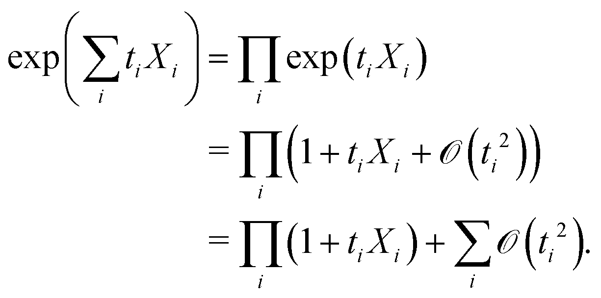 | (13) |
 | (14) |
 | (15) |
 | (16) |
 | (17) |
 term. Hence we will focus on contributions to it.
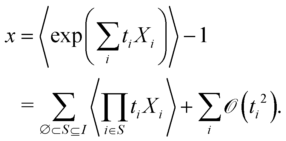
The first term, x, contains one subterm for each nonempty subset S of I. Only the subterm corresponding to S = I will be proportional to  . Its coefficient will then be
  .
.
The second term, −x2/2, contains when expanded one subterm for every ordered pair of nonempty subsets (S1,S2) of I. In order to get a term proportional to  each index i must be an element in exactly one of S1 and S2. In other words, {S1,S2} must be a partition of I. For every partition of I there are 2! matching ordered pairs, each contributing
  to the coefficient.
By now the rule for the kth term is clear. It will contain subterms corresponding to each partition of I into k nonempty sets. Each subterm will be a product of the prefactor (−1)k+1(k − 1)! and k expectation values.
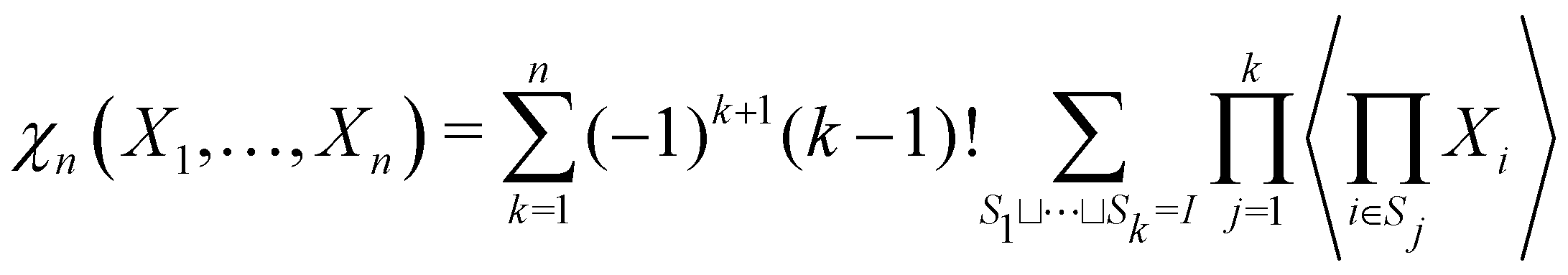 | (18) |
Conflicts of interest
There are no conflicts to declare.References
- L. J. Frasinski, Phys. Chem. Chem. Phys., 2022, 24, 20776–20787 RSC.
- V. Zhaunerchyk, L. Frasinski, J. H. Eland and R. Feifel, Phys. Rev. A: At., Mol., Opt. Phys., 2014, 89, 053418 CrossRef.
- A. Stuart and K. Ord, Kendall's advanced theory of statistics, distribution theory, John Wiley & Sons, 2010, vol. 1 Search PubMed.
Footnote |
| † Electronic supplementary information (ESI) available. See DOI: https://doi.org/10.1039/d3cp02525j |
| This journal is © the Owner Societies 2023 |