
Δ-Machine learning for quantum chemistry prediction of solution-phase molecular properties at the ground and excited states†
Xu
Chen
 ,
Pinyuan
Li
,
Eugen
Hruska
and
Fang
Liu
*
,
Pinyuan
Li
,
Eugen
Hruska
and
Fang
Liu
*
Department of Chemistry, Emory University, Atlanta, 30322, Georgia. E-mail: fang.liu@emory.edu
First published on 21st April 2023
Abstract
Due to the limitation of solvent models, quantum chemistry calculation of solution-phase molecular properties often deviates from experimental measurements. Recently, Δ-machine learning (Δ-ML) was shown to be a promising approach to correcting errors in the quantum chemistry calculation of solvated molecules. However, this approach's applicability to different molecular properties and its performance in various cases are still unknown. In this work, we tested the performance of Δ-ML in correcting redox potential and absorption energy calculations using four types of input descriptors and various ML methods. We sought to understand the dependence of Δ-ML performance on the property to predict the quantum chemistry method, the data set distribution/size, the type of input feature, and the feature selection techniques. We found that Δ-ML can effectively correct the errors in redox potentials calculated using density functional theory (DFT) and absorption energies calculated by time-dependent DFT. For both properties, the Δ-ML-corrected results showed less sensitivity to the DFT functional choice than the raw results. The optimal input descriptor depends on the property, regardless of the specific ML method used. The solvent–solute descriptor (SS) is the best for redox potential, whereas the combined molecular fingerprint (cFP) is the best for absorption energy. A detailed analysis of the feature space and the physical foundation of different descriptors well explained these observations. Feature selection did not further improve the Δ-ML performance. Finally, we analyzed the limitation of our Δ-ML solvent effect approach in data sets with molecules of varying degrees of electronic structure errors.
1 Introduction
The accurate and rapid prediction of chemical properties in the solution phase, where a large portion of real-life chemistry happens, is an essential step toward rational compound design and discovery.1–4 Although quantum mechanical (QM) methods combined with implicit and explicit solvent models have made significant progress to model solvated molecules,5–7 it is still challenging to make accurate predictions. In implicit solvent approaches, solvent molecules are treated implicitly as a polarizable continuum, and the solvation free energy is evaluated as the electrostatic interaction between the solute and the continuum plus some cavitation energy contribution. Such models are efficient but not accurate enough compared to experimental results. In contrast, explicit solvent models can produce more accurate results by treating the solvent explicitly and performing ensemble averages on solvation configurations sampled by molecular dynamics or Monte Carlo simulations. However, the higher computational costs related to configuration sampling8 and force field parameterization9 make it harder to be used for high-throughput prediction.In the last few years, machine learning (ML) has emerged as an invaluable tool to improve the efficiency and accuracy of molecular property prediction in the solution phase. ML can directly map a molecule structure to its property, leading to the rapid prediction of molecular properties at almost no computational costs compared to QM calculations. It has been used to predict the aqueous properties such as solvation free energy,10–12 photophysical properties,13,14 pKa,15etc. However, such ML models rely on the availability of large, high quality training sets of molecular properties in the solution phase, which are scarce compared to the many gas-phase molecular datasets available. The prediction is expected to have decent accuracy for molecules inside chemical space spanned by the training set molecules. For molecules with distinct chemistry from the training set, QM calculations are still needed.
A different approach to utilizing ML is to train models to improve the QM calculation accuracy. Such an idea, usually referred to as delta machine learning (Δ-ML), was originally introduced by Ramakrishnan et al.16 to improve the accuracy of gas-phase electronic structure calculations. For electronic structure calculations, most of the related physics has already been accounted in the low-level methods, such as density functional theory (DFT), but the correlation energy can only be accurately obtained from the computationally demanding high-level methods. Hence, by training a Δ-ML model to predict the electronic energy difference between the low-level and high-level methods, one can reach chemical accuracy at a low cost. Since the remaining deviations from reference results are typically smaller and possibly smoother, Δ-ML models have demonstrated unprecedented chemical accuracy and transferability.16 Δ-ML is recently generalized to QM calculations in the solution phase by different research groups, where the models were trained to predict the difference between the implicit solvent model calculated and experimentally measured properties in the solution phase. For example, Weinreich et al. built a Δ-ML model to predict solvation free energy and achieved an accuracy on par with state-of-the art physics-based approaches on the FreeSov dataset.11 Our recent work applying Δ-ML to reduce errors relative to experimental results in redox potential calculations has also exhibited improved accuracy compared to previously reported calculations without ML correction.17
Despite our previous successful application of Δ-ML in redox potential prediction, many fundamental questions remain to be answered. (1) Can this approach be generalized to improve excited-state molecular property prediction? (2) For other properties, how sensitive are the Δ-ML models to DFT functionals and ML method choice? (3) Which input descriptors are most suitable for the Δ-ML solution-phase property? (4) Does the optimal choice of descriptors depend on the property of interest, dataset size, or other facts about the dataset? (5) What are the limitations of this Δ-ML solvent effect approach? In this work, we aim to answer these questions by comparing Δ-ML models built based on four types of molecular descriptors. We will analyze the performance of the Δ-ML models for predicting a ground-state property, redox potential, and an excited-state property, UV/vis absorption energy. Detailed discussions will be made to answer the questions above.
2 Computational methods
2.1 Organization of data set
ML model training was carried out on two datasets of ground- and excited-state molecular properties in the solution phase. The ROP31318 data set was employed to test the performance of Δ-ML models for a representative ground-state property, redox potential. It is composed of 313 experimental redox potential records of organic and organometallic redox couples in four different solvents, including acetonitrile (MeCN, ε = 35.69), water (ε = 78.36), dichloromethane (ε = 8.93) and dimethylformamide (DMF, ε = 37.22). The computational redox potentials were calculated in our previous work17 using the Nernst equation: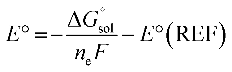 | (1) |
 is the free energy change of the reduced or oxidized process under standard conditions. ne is the number of electrons transferred in the process, which is 1 in our dataset. F is the Faraday constant. E°(REF) is the absolute potential of the ferrocene/ferrocenium (Fc+/Fc) redox couple, which is used as the internal reference for this dataset to reduce experimental19,20 and computational errors.21,22
 was estimated as:
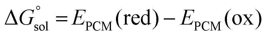 | (2) |
The refined optical absorption spectra (ROAS) data set was employed to test the performance of Δ-ML models for a representative excited-state property and the peak of solution-phase UV/vis absorption spectra is observed. The ROAS data set is a subset of the optical absorption spectra (OAS) data set,23 which contains 1447 individual molecules extracted from the auto-generated absorption energy database.23 We performed time-dependent density functional theory (TDDFT) calculations in the implicit solvent on the OAS data set to obtain the computational absorption energies. To ensure the quality of the Δ-ML model training, we carefully refined the OAS data set by excluding records with high uncertainties. The excluded records include 15 single atom structures with a disproportionately large difference between experimental and computational results, 28 incorrect molecular information, 4 molecules with TDDFT convergence problems, 4 molecules without available experimental data and 1 molecule containing 5th row transition metals (list available in Figshare).24 After cleaning the dataset, we obtained 1395 valid unique records in nine solvents. This refined dataset possesses molecules with the number of atoms ranging from 2 to 242 and total electrons ranging from 18 to 922 (Table 1). The types of molecules include simple inorganic compounds (such as sodium methoxide), organic compounds, and organometallic compounds.
| Redox potential (313) | Absorption energy | ||
|---|---|---|---|
| OROP (193) | OMROP (120) | ROAS (1395) | |
| Metal | None | Ni, Mn, Co, Cr, Rh, Ru, Ti, Os, Fe, Ir | In, Ag, Ti, Se, Fe, Ru, Cd, Zn, Mg |
| Charge | −2 to 2 | −3 to 3 | 0 |
| Spin | 1 and 2 | 1 to 6 | 1 |
| Size | 5 to 82 | 13 to 79 | 2 to 242 |
| Solvent type | 2 | 4 | 9 |
| Notation | E° | E abs | |
2.2 DFT calculation methods
TeraChem quantum chemistry software25 was used to perform all geometry optimizations and single-point energy calculations. Solution-phase geometry optimizations were carried out using a TRIC optimizer26 with the default tolerance of 4.5 × 10⁻⁴ hartree per bohr for the maximum gradient and 1 × 10⁻⁶ hartree for the change in self-consistent field (SCF) energy between steps. We used the conductor-like polarizable continuum model (C-PCM), implemented in TeraChem,5,27 for all solution-phase calculations. The solute cavity was built using default Bondi's van der Waals radii28 for available nonmetal elements in TeraChem, standard van der Waals radii from the literature29 for metals, both scaled by a factor of 1.2 and a default PCM cavity density (17–110 points per atom).For the geometry optimization calculations of redox potential, we used an optimal functional/basis set combination shown in our previous paper,17 including the B3LYP functional with the DFT-D3 empirical dispersion correction, combined with LANL2DZ30 effective core potentials for the transition metals, I, or Br and the 6-31G* basis for the remaining. To test the sensitivity of different ML models for various DFT functionals, we used the B3LYP optimized geometries but a series of range-corrected hybrid (ωB97,31 ωB97X,31 ωPBEh,32 CAM-B3LYP)33 and hybrid (B3LYP,34 PBE0)35 functionals with D3 van der Waals corrections36 to calculate single-point energies to obtain redox potentials. The standard range-separation parameters, ω = 0.2 bohr−1 and ω = 0.3 bohr−1, were used for ωPBEh and CAM-B3LYP functionals, respectively.
For absorption energy calculations in the solution phase, we performed time-dependent density functional theory (TDDFT) calculation with Tamm-Dancoff approximation (TDA),37 with non-equilibrium solvation treated with the linear response polarizable continuum model (LR-PCM).38 For each molecule, the solute geometry was first optimized at the ground state with DFT, followed by LR-PCM TDA calculation with the respective DFT functional to obtain the excitation energies and oscillator strengths of the ten lowest singlet excited states. A closed shell Kohn–Sham reference is always used because all molecules in the ROAS dataset have singlet ground states. A broadened spectrum was then generated by convoluting the stick spectra with a Gaussian function of a full width at half maximum (FWHM) of 0.25 eV. The peak absorption energy of the convoluted spectrum was read out to be compared with the experimental spectrum peak. To test the sensitivity of ML models, the calculations were also repeated for a set of exchange-correlation (XC) functionals (B3LYP, PBE0, ωB97, ωB97X, ωPBEh with ω = 0.2 bohr−1, CAM-B3LYP with ω = 0.3 bohr−1), with the basis set kept the same as used in redox potential calculations. For each ROAS record, the solvent static dielectric constant, ε, and the “fast” or optical dielectric constant, ε∞, were obtained from the literature,39 with ε∞ calculated as the square of the solvent's refractive index.
2.3 Machine learning models
We investigated the performance of ML models to correct errors in redox potential and absorption energy calculations. We tested four types of molecular descriptors as input features and the calculation errors as the output. Different types of ML models were trained with scikit-learn,40 including linear (lin) regression, random forest (RF) regression, gradient boost (GB) regression, kernel ridge regression (KRR), and artificial neural network (ANN). The input features were first normalized to have zero mean and unit variance. The data set was then randomly split into a training set (80%) and a test set (20%). The hyperparameters for all models were tuned using Hyperopt41 by 5-fold cross-validation on the training set (Table S1, ESI†), i.e., 64% of overall data as the sub-training set and 16% of overall data as the validation set. With the optimized hyperparameters, the model's performance was then evaluated by retraining the whole training set while predicting the test set. The mean absolute error (MAE) was used to gauge all the performance.2.4 Multi-reference character analysis
We performed the multi-reference (MR) diagnostic on the OMROP data set by using the open-source toolkit, MultirefPredict.42 Specifically, rND diagnostics,43,44 the ratio of the static correlation to the total correlation (i.e., static and dynamical correlation), has been applied to reflect MR character of a molecule. Both static and dynamical correlation can be efficiently obtained from finite-temperature DFT (FT-DFT)45 calculations. All the DFT calculations that employed the PBE46 functional with the basis set remained the same as used in redox potential calculations. The FT-DFT calculations employed the recommended47 temperature for PBE (5000 K) with Fermi–Dirac smearing.3 Feature construction
In order to correct the errors in solution-phase property calculations, the information encoded in the error source needs to be converted into an appropriate number of input features. Unlike gas-phase property predictions, where errors can only come from the electronic structure methods and experimental measurements,48 solvent models can also potentially contribute to errors in solution-phase property predictions. Due to the limited size of our data set, we focused on the classes of features meeting the criteria of (1) providing expressive information for both the solute and the solvent and (2) satisfying requirements of low dimensionality and low cost of acquiring.49 Specifically, we tested the following four types of descriptors for solvated molecules (Fig. 1):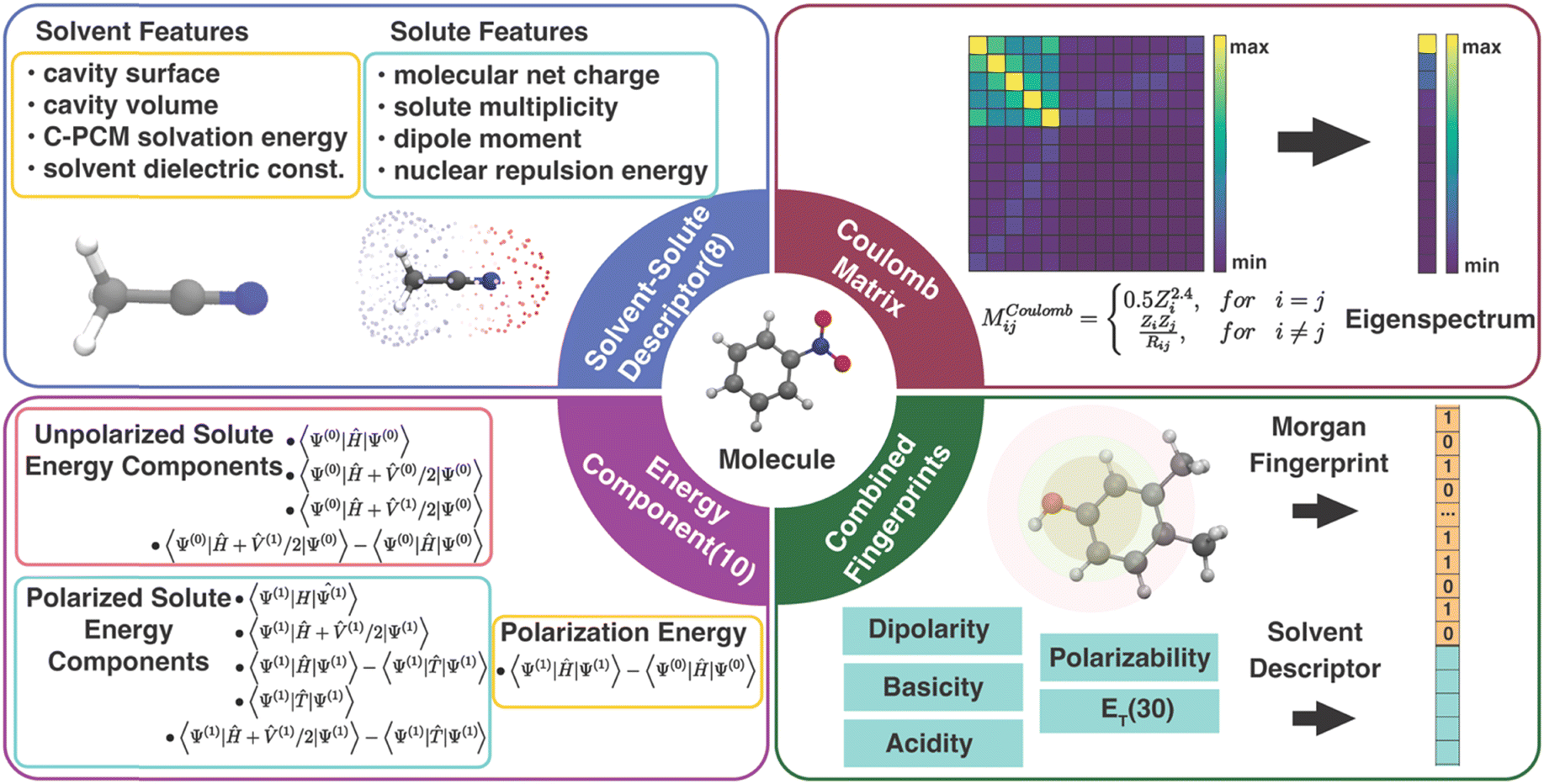 | ||
| Fig. 1 Diagram of four types of descriptors for solvated molecules. | ||
3.1 Physics-inspired solute and solvent descriptors
The solute and solvent (SS) descriptor is a physically inspired descriptor for solvent–solute interactions in molecular systems. It was first introduced in our work for correcting the errors in redox potential calculation17 and will also be used to correct the errors in calculated solution-phase UV/vis absorption energy in this work. The solute net charge, dipole moment, spin multiplicity, and nuclear repulsion energy of the molecule are included to describe the solute molecule. The solvent is described by the implicit solvation cavity surface area and volume, PCM solvation energy, and the dielectric constant.3.2 Energy component descriptors
The components of the solvent–solute interaction energy in the PCM were used by Alibakhshi et al.12 as input features of ML models to predict the solvation free energy in the ML PCM model. We extracted 10 energy components (EC) from the original 15 well-defined PCM energy components to avoid overlapping with the SS descriptor (calculation details in Text S1 and Table S2, ESI†). These 10 features encode various types of interactions in quantum chemistry calculations of a solute molecule in a PCM field, including the total energy of an unpolarized solute without a PCM field and with a polarized or unpolarized PCM field, the total energy of a polarized solute with and without a PCM field, the interaction energy of the unpolarized solute and polarized solvent, the solute polarization energy, the total potential energy, the total kinetic energy, and the solvation free energy. In our interpretation, some EC features are linearly dependent, e.g., the polarization energy is equal to the difference between the total energy of a polarized solute without a PCM field and an unpolarized solute without a PCM field. As a result, the 10 energy components can be further reduced to 6 components by removing the redundant descriptors without affecting the ML performance (Table S3, ESI†). However, all EC models in this work were trained with the 10 features to be consistent with the original EC definition by Alibakhshi et al.123.3 Coulomb matrix
Coulomb matrix (CM) is a class of widely used molecular geometric features leading to well-performing models of molecular properties.50–52 The matrix elements of CM are given by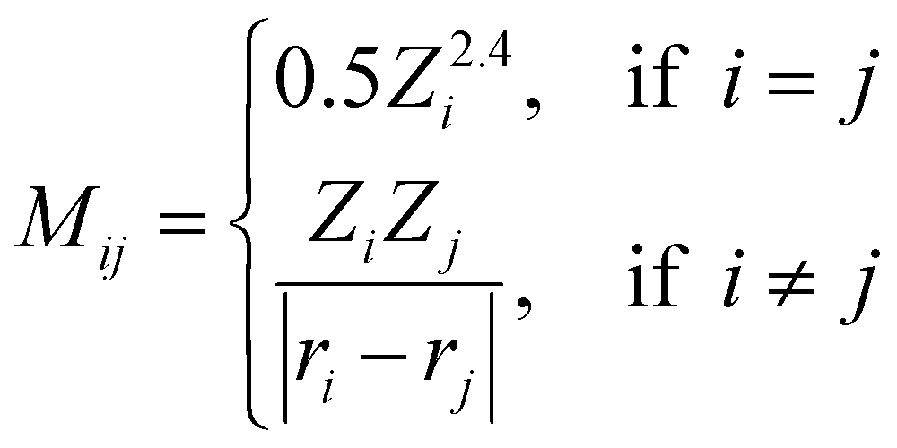 | (3) |
3.4 Molecular fingerprints
Molecular fingerprints were initially designed for substructure searching in chemical databases and were later used for analysis tasks, such as similarity searching in virtual screening.54,55 Modern implementations [e.g., extended-connectivity fingerprints (ECFPs)] designed to encode molecular features relevant to molecular activity have recently been proven well-suited as input features for ML models.14,56 Here, we proposed a combined fingerprint descriptor (cFP) that describes the solute with Morgan fingerprint57 (also known as ECFP4) and the solvent with ET(30)58 along with four other empirical scales (dipolarity, polarizability, acidity, and basicity).59 The Morgan fingerprint (FP), as one of the best-performing fingerprints among small molecules, can perceive the circular substructure around each atom in a solute molecule. Considering the size of our data sets, the Morgan fingerprint used in cFP was generated by RDKit60 of 128, 64, and 1024 bits for OROP, OMROP, and ROAS, respectively.When training Δ-ML models, the raw QM calculated molecular property is always added to each of the aforementioned molecular descriptors to form the input feature. The reason is that the raw QM calculated result is the crude estimator of the property (CEP), which has been shown to be a crucial input feature in ML chemistry studies with small training sets.61 The raw QM calculated result also has a high feature importance score in our previous study.17 The ML performance without adding the CEP has also been noted (Tables S4–S6, ESI†). Our results reveal that the lowest MAE of the Δ-ML models, considering all descriptors and ML model combinations, increased by 228% and 34% for predictions on OROP and ROAS datasets, respectively. Additionally, when the raw QM result input was removed, these models exhibited limited predictive ability on OMROP data.
4 Result and discussion
In the following sections, we will analyze the performance of the four types of molecular descriptors on both redox potential and absorption energy corrections. Specifically, we intend to answer the following questions:1. Which types of descriptors have the best performance for Δ-ML models to correct errors in quantum chemistry calculation of solution-phase molecular properties?
2. Does the optimal choice of descriptors depend on the predicted molecular property, dataset size, or other factors about the dataset?
3. How sensitive are the Δ-ML models to DFT functionals and ML method choice?
4. What are the limitations of this Δ-ML solvent effects approach?
4.1 Δ-ML for redox potential
Recent work in our group17 has shown that the SS descriptor can efficiently encode solvent–solute information to correct the redox potential calculation errors, which are believed to be mainly caused by C-PCM's imbalanced treatment of differently charged species. In that work, the PBE0-D3 functional combined with corrections of KRR and RF can generate the best correction results for OROP and OMROP sets, respectively. Herein, we seek to understand whether other types of descriptors (CM, EC, and cFP) can outperform SS for the Δ-ML redox potential. As the first step, we kept our previous choice of the optimal DFT functional (PBE0-D3) and optimal ML methods (KRR for OROP and RF for OMROP) and compared the Δ-ML performance of the four descriptors. As shown in Fig. 2, all four types of descriptors can greatly reduce the errors, reducing the MAE from 0.263 V to less than 0.200 V for OROP, and from 0.817 V to less than 0.577 for OMROP. For OROP corrected with KRR, the MAE of CM (0.163 V) is only marginally better than the other three descriptors by up to 0.04 V.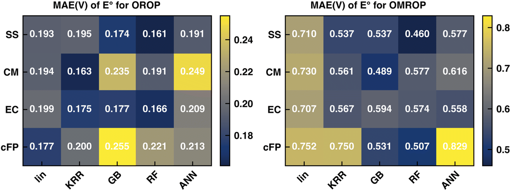 | ||
| Fig. 2 Test set MAE of the Δ-ML corrected redox potential (calculated with PBE0-D3 functional) for (left) OROP and (right) OMROP datasets. The Δ-ML models were trained with different combinations of descriptors and ML models. | ||
Similarly, for OMROP corrected with RF, the best-performing SS descriptor is only slightly better than the others in MAE by 0.04–0.12 V. Since the Δ-ML performance depends on the choice of the descriptor (how efficiently the local environments can be encoded) and the ML framework (the functional flexibility in mapping descriptors to outputs), we then varied the ML methods to investigate the impacts. We compared the descriptors by their performance when combined with the respective optimal ML method. We also compared the variations of performance caused by different ML methods. SS has the best performance when combined with RF, for both OROP (MAE: 0.161 V) and OMROP (MAE: 0.460 V). Furthermore, SS has the most stable performance, as its worst-case scenario is always better than that of the other descriptors. In summary, SS has the best performance for the Δ-ML redox potential on the tested data sets, although the performance difference among different descriptors is not significant.
4.2 Δ-ML for absorption energy
Although the SS descriptor has shown the overall best performance in correcting the calculated redox potential, it remains unknown whether it is also the best descriptor for Δ-ML of other chemical properties. To answer this question, we applied the same Δ-ML strategy to correct the calculated absorption energies of the ROAS dataset and compare the performance of the four types of descriptors. Traditionally, the calculated absorption energies of a dataset are corrected by first categorizing the dataset into a few groups, such as according to their chromophoric unit62 or ground-state electronic configurations,63 and then using linear regression for the respective groups. Although such a method can provide relatively accurate results on an organic dye dataset with less than a hundred data points,62,63 it may be less effective for larger and more diverse data sets.Here, we investigated the Δ-ML performance on ROAS, a diverse set with ca. 1400 organic dyes. As the starting point, we fixed the XC functional used in the TD-DFT/TDA calculations of absorption energies and investigated the Δ-ML performance of different descriptors in combination with different ML methods. Here, the PBE0 functional was used due to its decent estimation for organic's electronic transition energies at low cost.62 Discussions about other XC functionals (e.g., range-corrected hybrids) will be covered in Section 4.3. As shown in Fig. 3, the raw calculated absorption energies of the ROAS dataset have a systematic overestimation and many big-error outliers. The Δ-ML results (cFP descriptor combined with GB) distribute more evenly on both sides of the diagonal of the parity plot. Both the systematic and the outlier errors are greatly alleviated, resulting in significantly reduced MAE. All Δ-ML models can significantly reduce the MAE by more than 34%, regardless of the descriptors or ML methods (Tables S7–S10, ESI†). In contrast to the Δ-ML redox potential results, we can see a significant performance dependence on the descriptor choice. The cFP descriptor has its best-case performance (combined with GB, MAE: 0.318 eV) significantly better than others (MAE: 0.437–0.501 eV), and even its worst-case performance (combined with the linear model, MAE: 0.463 eV) is still close to or better than CM and EC's best-case performance (Table 2).
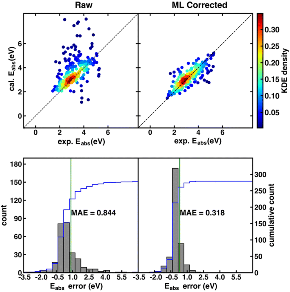 | ||
| Fig. 3 (top) Parity plots of the PBE0 calculated vs. experimental Eabs. Top left: Raw data from TD-DFT/TDA calculations. Top right: Δ-ML corrected data obtained with the best-performing cFP descriptor combined with the GB model. As indicated by the color bar on the right, data points are colored by kernel density estimation (KDE) density values. (bottom) Histograms of errors of the Eabs before (bottom left) and after Δ-ML correction (bottom right). | ||
| MAE (eV) | Raw | Linear | KRR | GB | RF | ANN | Best reduction (%) |
|---|---|---|---|---|---|---|---|
| SS | 0.844 | 0.586 | 0.460 | 0.460 | 0.437 | 0.518 | 48.2 |
| CM | 0.596 | 0.458 | 0.477 | 0.462 | 0.570 | 45.7 | |
| EC | 0.604 | 0.521 | 0.501 | 0.510 | 0.527 | 40.6 | |
| cFP | 0.463 | 0.394 | 0.318 | 0.330 | 0.442 | 62.3 |
4.3 Sensitivity of Δ-ML to DFT functional choices
This section discusses the sensitivity of Δ-ML performance on computational data sets calculated with various XC functionals. The choice of XC functionals is known to strongly influence the accuracy of redox potential and absorption energy calculations in the implicit solvent.62,64 As a result, the optimal range-correction parameter of long-range corrected XC functionals needs to be tuned case by case, making it hard to accurately predict a large and diverse dataset using a single fixed XC functional. In our previous work,17 we already saw the large variation in MAE for the redox potential calculations by different functionals (0.263–0.618 V for OROP, 0.817–1.573 V for OMROP) and that Δ-ML corrected results (SS descriptor combined with KRR) had significantly less sensitivity to XC functional choice. Here, we further tested: (1) whether Δ-ML also reduces the functional sensitivity in DFT calculations of other properties, such as the absorption energy and (2) whether Δ-ML using other descriptors also reduces the sensitivity to functional choice.Our result shows that the performance of different functionals in predicting redox potentials varied significantly (Fig. 4 left). For the OROP dataset, the PBE0-D3 functional achieved the lowest MAE of 0.263 V, while the ωB97-D3 functional had the highest MAE of 0.618 V, resulting in a difference of 0.355 V (Tables S11–S14, ESI†). For the OMROP dataset, the best-performing PBE0-D3 functional had an MAE of 0.817 V, while the ωPBEh-D3 functional had the highest MAE of 1.573 V, resulting in a difference of 0.756 V (Tables S15–S18, ESI†). For the absorption energy calculation, the MAE of the best-performing B3LYP (0.787 eV) differs from the worst ωPBEh (1.119 eV) by 0.332 eV (Tables S7–S10, ESI†). In contrast, utilizing ML models to correct the calculations is less sensitive to DFT functional choice regardless of the descriptors used for both redox potential and absorption energy predictions (Fig. 4 right). All the ML models can greatly reduce the MAE, and the accuracy of the ML corrected result is not directly related to the original MAE. Instead, the improvement is affected by the data distribution, ML models, and descriptors. For example, although the MAE of absorption energy calculated by B3LYP is the best among all functionals, it becomes the worst in many cases after ML corrections.
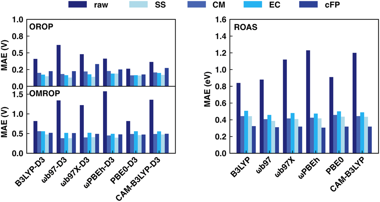 | ||
| Fig. 4 Comparison of MAE for redox potential (left) and absorption energy (right) correction before and after Δ-ML for various descriptors and DFT functionals. For each functional using each type of descriptor, the best-performing ML method's results are reported. OROP (top left) and OMROP (bottom left) data sets were used to test redox potential prediction (in V), whereas the ROAS dataset was used for absorption energy prediction (in eV). | ||
In general, RF and GB are the most suitable ML models for all DFT functionals and descriptor choices, with a few exceptions when using CM and cFP as descriptors. Based on the overall performance using various ML models, the best descriptor for redox potential prediction is SS (OROP: ωB97-D3 combined with GB, MAE: 0.131 V; OMROP: ωB97-D3 combined with GB, MAE: 0.381), whereas the best descriptor for absorption energy is cFP (ωPBEh combined with GB, MAE: 0.306 eV). Although the DFT functional choice has less impact after ML correction, ωB97, ωPBEh, and PBE0 are overall the best after ML corrections across all the data sets. Therefore, ωB97 calculated results were used in later sections’ analysis if not specified.
4.4 Interpretation of the impact of descriptors on Δ-ML performance
We first applied principal component analysis (PCA) to understand how well the datasets are represented in the feature space spanned by different descriptors. (Fig. 5). In general, the feature space with more evenly distributed data points and apparent clustering of ΔE° (or ΔEabs) has greater ML predictability. For the OROP data set, SS and EC are more predictive than CM, where data points are not well separated. Although cFP projection has well-separated data points and a gradually varying ΔE° along the PC1 direction, it has a relatively bad Δ-ML performance. It is likely due to the low ratio (35%) of the feature space variance encoded in the first two components of cFP, in contrast to SS, CM, and EC, where the majority of feature space variation (over 92%) can be encoded into PC1 and PC2. For the OMROP data set, EC and cFP both present a string-like distribution with little separation of data along one of the principal components, leading to a worse performance compared to the SS descriptor. As for ROAS, although cFP still has the string-like distribution as in OMROP, the strings are more evenly distributed in the PC1 direction, and the ΔEabs can be well distinguished along the PC2 direction. These observations in PCA can partially explain the varying of performance for different descriptors in different data sets.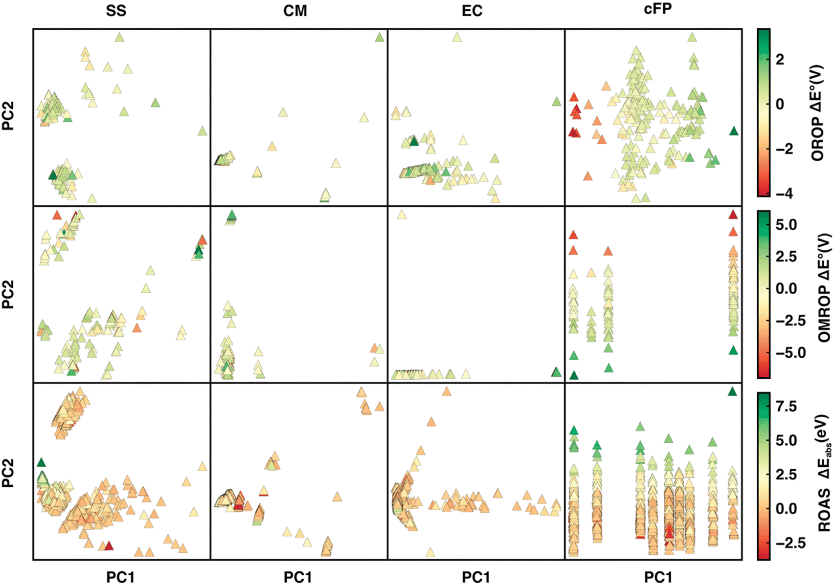 | ||
| Fig. 5 Projection of OROP, OMROP, and ROAS data sets (from the first to the third row of panels) onto the first two principal components for the SS, CM, EC, cFP descriptors. The PCA plots are colored by the ωb97(-D3) calculation error with respect to the experimental results. | ||
We then sought the physical explanation for the performance variation of different descriptors when applied to different datasets. The reason for SS's better performance in correcting errors in redox potential than absorption energy is likely to be the different molecule characters in the two data sets. The ROAS data set contains only neutral spin-singlet species. As a result, the charge and spin feature in SS will be ineffective for ROAS. The all-neutral species will also lead to a significantly narrower range of solvation energy distribution (Fig. 6) because the C-PCM solvation energy magnitude depends on the net charge of the solute. Therefore, it is even harder for an ML model to map SS to the target absorption energy. Similarly, we can explain the poorer performance of EC descriptors when applied to correcting excitation energies of ROAS data sets. The energy components of EC are extracted from the ground-state equilibrium solvent calculations and thus lack the direct description of the non-equilibrium solvation process upon excitation. In addition, neither SS nor EC provides as much molecular structure information as cFP, which can also be critical for encoding excited-state properties.14
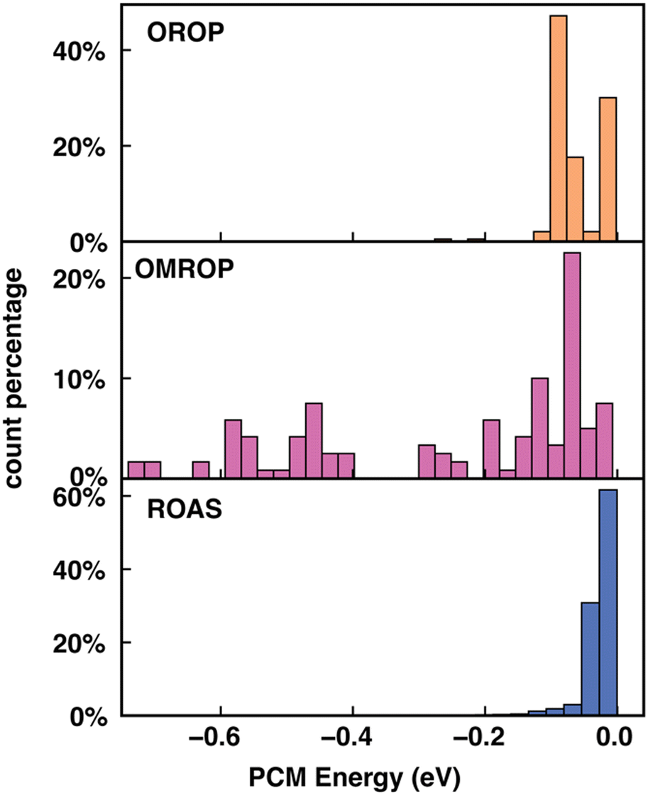 | ||
| Fig. 6 C-PCM solvation energy (in eV) distribution for OROP, OMROP and ROAS. | ||
4.5 Impacts of feature selection
In previous sections, we have seen the limitations of the four types of descriptors for correcting different properties for our Δ-ML solvent effects approach. This inspires the fine-tuning of the feature set to improve the Δ-ML performance further. It is known that performing feature selection can decrease the training complexity and time for nonlinear models and increase the model stability, transferability, and out-of-sample performance for linear models.65 Based on the characters of our three benchmark datasets and the molecular property to predict, we tested three different feature selection strategies as elaborated below.First, for the Δ-ML redox potential on the OROP and OMROP set, SS descriptors have already shown decent performance (Section 4.1). Hence, we sought to further improve the performance by using a hybrid feature set combining SS with different types of descriptors. The random forest-ranked recursive feature addition (RF-RFA)65 was used to select features from SS and EC descriptors. CM and cFP were not included in RF-RFA because they both encode the geometric information of a whole molecule and are not physically very meaningful to be partially selected as features in an additive manner. To perform RF-RFA, we first combined the SS and EC descriptors and ranked them with the RF feature importance scores. The raw calculated redox potential was set as the initial feature due to its highest importance score, whereas other SS and EC descriptors were added at a time based on ranking. During each feature addition cycle, the ML model was retrained with hyper-parameter tuning, with the performance evaluated by a 5-fold cross-validation score (CVS). The RF-RFA was stopped when no improvement in the validation score (MAE) was observed (Tables S19 and S20, ESI†). Only the ANN model trained on OROP got a significantly smaller MAE of 0.155 V after feature selection, compared to the original MAE of 0.253 V. All other ML models did not benefit much from the feature selection process.
Second, for the Δ-ML absorption energy, cFP, the descriptor composed of Morgan FP plus some additional features for the solvent, has the best performance. Here, we focus on optimizing the length of Morgan FP used in cFP. Since the previously reported optimal Morgan FP length varies based on the training sets,56,66,67 our model using 1024 bits of Morgan FP may not reach its best performance. Considering our dataset size (1395), we restricted the range of Morgan FP length to no more than 1024 bits to avoid overfitting caused by the high dimension of the descriptor. We compared the performance of cFP composed of Morgan FP of different lengths generated in two approaches. In the first approach, we used RDKit to generate Morgan FP of 1024, 512, 256, and 128 bits. In the second approach, we generated a long Morgan FP with 3072 bits, whose dimension is then reduced to 1024, 512, 256, and 128 bits using the univariate feature selection method, “SelectKBest”, in scikit-learn.68 We found that for the same length of bits, the cFP generated with the second approach (dimension reduction) has worse performance than the cFP generated by the first approach (direct generation) (Tables S21 and S22, ESI†). For the directly generated cFP, the best-performing one has 1024 bits, which happened to be the length we initially selected.
Third, we further tested whether the performance of the Δ-ML absorption energy can be further improved by adding SS or EC features to cFP. This strategy still did not present a significantly better outcome. A detailed description of this method and results can be found in the ESI† Text S2 and Table S23.
All the final performances after feature selection were evaluated by training on the full training set (80% of the whole data set) and testing on the set-aside test set (20%). The above results indicate that additional feature engineering is not necessary in our cases. One possible reason is that the chemical information encoded by different descriptors may be similar. Besides, the inherent regularization methods (e.g., the L2 regularization in KRR) may have already prevented the model from overfitting.
4.6 Dependence of Δ-ML performance on data set size
We then looked into the potential dependence of different descriptors’ Δ-ML performance on training set size, which helps us understand the applicability of different descriptors for differently sized datasets. The training set size dependence was tested on all three data sets (OROP, OMROP, and ROAS). For each data set, 20% data were set aside as the test set and the rest data (80%) as the training set. A series of sub-training sets were then formed by extracting different portions of data from the training set (20–100% training, or 16–80% total). RF models were then trained based on these sub-training sets using various descriptors as input features (Fig. 7) but were always tested on the same test set (20% total).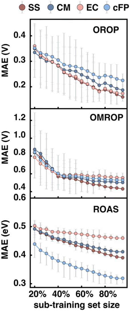 | ||
| Fig. 7 Change of MAE with the increase of training set portion for different descriptors and data sets (top: OROP, middle: OMROP, bottom: ROAS) using ωB97 for DFT or TDDFT calculation and RF for Δ-ML. For each data point on the plot with sub-training set size X%, the sub-training set was formed by randomly selecting X% data from the full training set (80% total) and was trained and predicted on the fixed set-aside test set (20% total). For each data point, the random selection of the sub-training set was repeated ten times. Each color dot shows the average performance (MAE) of the ten tests, with the error bar indicating the highest and lowest MAE. | ||
As the sub-training set size increases, the Δ-ML performance improves for almost all models, regardless of the targeting property (redox potential or absorption energy) or the descriptors used. However, for models trained on OMROP, the improvement slows down significantly after the sub-training set size reaches 40% (or 32% total). This phenomenon is especially prominent for the EC descriptors, where the curve reaches a plateau for sub-training set size >40%. A similar issue is seen for the ROAS data set, where the EC slope is much flatter than other descriptors. One possible explanation for these results is that the EC descriptor may not be sufficiently expressive for accurately predicting calculation errors in OMROP and ROAS datasets. As a result, the model may have reached its capacity quickly and experienced underfitting, where it fails to capture the underlying patterns in the data. Increasing the training data further may not lead to significant improvement in the Δ-ML performance.
For each data set, the relative performance of different input descriptors can change as the training set size increases. For the Δ-ML redox potential (OROP and OMROP sets), CM or EC has the best performance when trained with fewer data (<40%), but SS outperforms all others when more training data become available (≥40%). However, such a change of relative performance is not seen for Δ-ML absorption energy (ROAS), where the cFP descriptor always has the best performance regardless of the training set size.
4.7 Limitations of the Δ-ML solvent effects approach
The error in calculated solution-phase properties compared to experimental results is mainly attributed to the inaccuracy of solvent models and the approximate electronic structure methods. Although the errors of solvent models can potentially be fixed by Δ-ML with solvent–solute interaction descriptors as input features, the electronic structure errors are harder to be encoded by our descriptors. Such a drawback is expected to be more prominent when the electronic structure error dominates, such as in transition-metal-containing systems69,70 or electronically excited molecules.For transition metal complexes, the prevalent degenerate orbitals (d or f orbitals) lead to a significant multireference character of their electronic structure, which cannot be accurately described by Kohn–Sham DFT.71 The strength of multireference character varies in different transition metal complexes. We hypothesize that our Δ-ML approach may have worse performance in molecules with significant multireference characters, where electronic structure errors dominate over solvent model errors. To test our hypothesis, we carried out the MR character analysis72 on the OMROP data set, trying to correlate the Δ-ML performance with the MR diagnostic values. The specific MR diagnostic used is the rND diagnostics, as described in Section 2.4. We used the ratio between the calculation error after (eML) and before (eraw) Δ-ML correction to quantify the Δ-ML performance (Fig. 8). Hence, 0 < eML/eraw < 1 indicates an improved result after Δ-ML; −1 < eML/eraw <0 indicates a slight overcorrection, but the absolute error is still reduced; eML/eraw > 1 indicates a worse result; and eML/eraw < −1 indicates a severely overcorrected result. To our surprise, the overall Δ-ML performance is better for molecules with more MR character (rND > 0.3), because the Δ-ML models significantly overcorrect the E° error in some lower-MR-character molecules. A possible reason is that our Δ-ML approach empirically corrects all errors in the calculated results relative to experiments, including both electronic structure and solvation errors. The OMROP data set has more molecules (67%) with high MR-character, so the trained Δ-ML models bias towards appropriately correcting high-MR systems but overcorrecting the low-MR molecules. A potential solution to this problem is to develop separate Δ-ML models for correcting electronic structure errors and solvent model errors. However, this is beyond the scope of this work and will be investigated in the future.
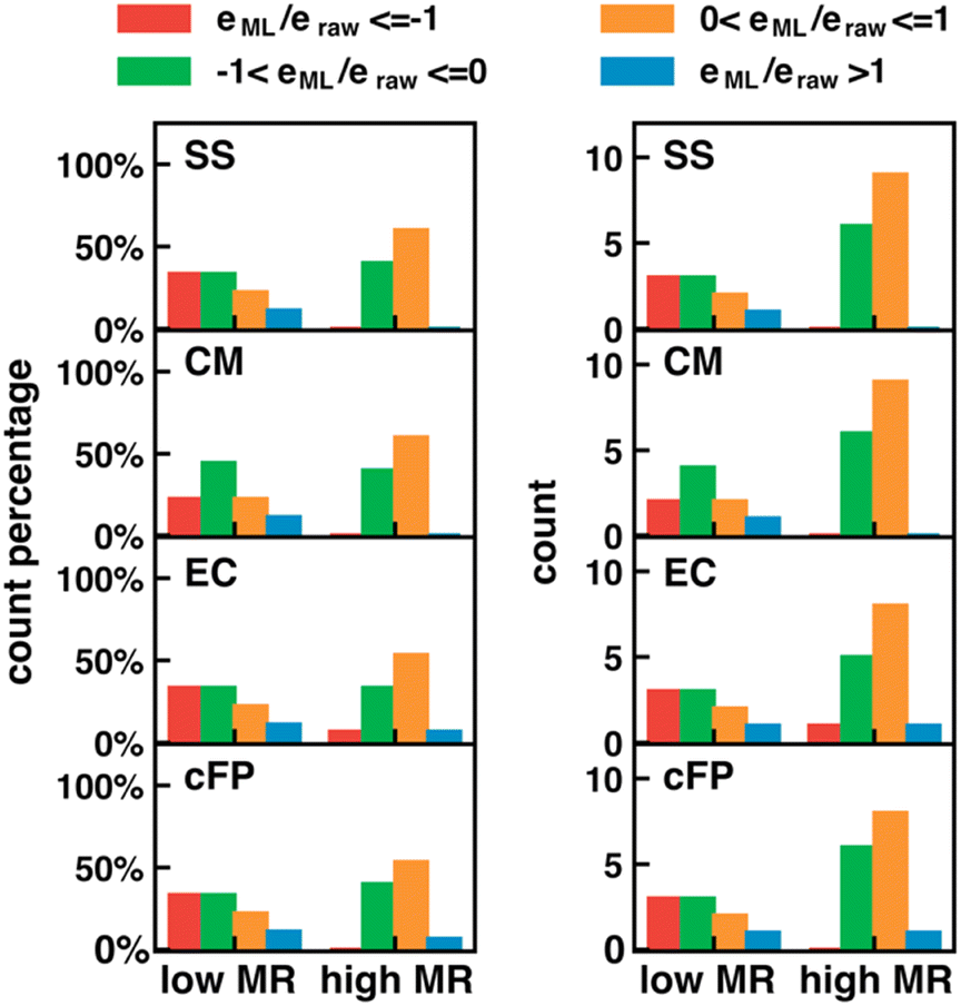 | ||
| Fig. 8 Dependence of Δ-ML performance on the multireference (MR) character of the molecules. Δ-ML performance is measured by the ratio, eML/eraw, for the errors before and after Δ-ML. The clustered bar charts show the normalized distribution (left) and direct count (right) of molecules with eML/eraw in different ranges. (−∞if−1]: red, (−1,0]: green, (0,1]: orange, (1, ∞): blue. In each panel, the statistics was obtained separately for molecules with low MR characters (rND < 0.3) and high MR characters (rND ≥ 0.3), where rND was calculated using the PBE functional at 5000 K. Each row of panels is the result of one type of descriptor (SS, CM, EC, or cFP from top to bottom). | ||
5 Conclusions
This work exploits the Δ-ML solvent effect approach to reduce the errors in DFT-calculated solution-phase molecular properties compared to experimental measurements. We sought to understand the dependence of Δ-ML performance on the type of molecular property to predict the ground or excited-state, the type of input descriptor (SS, CM, EC, and cFP), data set distribution, data set size, and feature selection.For the prediction of the ground-state redox potential of organic compounds (OROP data set), the SS, EC, and CM descriptors demonstrated a better performance than cFP. For the OMROP data set composed of organometallic compounds, the SS descriptor was the best descriptor. The transferability of the Δ-ML approach to excited-state properties was then tested on the ROAS data set of solution-phase UV/vis absorption spectra, for which the cFP descriptor had the best predictivity. Δ-ML always reduces the sensitivity of calculated properties to DFT functional choice, no matter which descriptor or ML model was used. We then analyzed why the optimal descriptor depends on the type of property to predict and data distribution. PCA analysis showed that the distribution of data in different feature spaces impacted the Δ-ML performance. Additionally, we analyzed based on the physical foundation of various descriptors. The SS descriptor is expected to have better performance for data sets with diverse net charges, whereas cFP is expected to be better at distinguishing neutral molecules. The EC descriptor is obtained from ground state molecules in equilibrium solvation and cannot give satisfactory predictions for absorption energy, which depends on excited states in non-equilibrium solvation.
We also investigated the dependence of Δ-ML performance on the data set size. As the training set size increased, overfitting happened for a few cases where the chosen descriptor could not encode the variation in the data well. Typical examples are the Δ-ML models using the EC descriptor on OMROP and ROAS data sets.
Furthermore, we sought to optimize the feature set using different feature-engineering strategies, including RF-RFA and SelectKBest. None of them resulted in a better Δ-ML performance (in terms of MAE) than directly using the best-performing feature set.
Finally, we analyzed the limitation of our Δ-ML solvent effect approach. Although developed to correct errors caused by the inaccuracy of solvent models, our Δ-ML models empirically corrected all types of errors in the calculated properties, including electronic structure errors. For a diverse data set like OMROP, our Δ-ML approach may be biased towards correcting electronic structure-related errors in molecules with significant multireference character and therefore overcorrecting other molecules. This motivates future developments of a multiple-step Δ-ML approach that corrects electronic structure errors and solvent effect-related errors separately.
Data availability
Data for this paper, including detailed information and optimized structures of ROAS data set, feature input, and trained ML models are available at Figshare at https://figshare.com/articles/dataset/SI_data_ml-representation_paper/21986717.Author contributions
X. C. is responsible for the investigation, methodology, programming, formal analysis, visualization, and writing. P. L. contributed to the data curation. E. H. contributed to part of the computer code, supporting algorithms and data analysis. F. L. contributed to the conceptualization, funding acquisition, supervision and writing review and editing.Conflicts of interest
There are no conflicts to declare.Acknowledgements
The authors acknowledge the Donors of the American Chemical Society Petroleum Research Fund for the support of this research through grant number PRF #65858-DNI4. Financial support for this publication partially results from Scialog grants #28789 and #28755 from Research Corporation for Science Advancement. This work used the Extreme Science and Engineering Discovery Environment (XSEDE)73 Bridges-2 at Pittsburgh Supercomputing Center through allocation CHE210036, which is supported by National Science Foundation grant number ACI-1548562.Notes and references
- A. Jinich, B. Sanchez-Lengeling, H. Ren, R. Harman and A. Aspuru-Guzik, ACS Cent. Sci., 2019, 5, 1199–1210 CrossRef CAS PubMed.
- J. Liu, X. Wang, J. Z. Zhang and X. He, RSC Adv., 2015, 5, 107020 RSC.
- R. Skyner, J. McDonagh, C. Groom, T. Van Mourik and J. Mitchell, Phys. Chem. Chem. Phys., 2015, 17, 6174–6191 RSC.
- B. Meredig, A. Agrawal, S. Kirklin, J. E. Saal, J. W. Doak, A. Thompson, K. Zhang, A. Choudhary and C. Wolverton, Phys. Rev. B: Condens. Matter Mater. Phys., 2014, 89, 094104 CrossRef.
- F. Liu, N. Luehr, H. J. Kulik and T. J. Martínez, J. Chem. Theory Comput., 2015, 11, 3131–3144 CrossRef CAS PubMed.
- J. Zhang, H. Zhang, T. Wu, Q. Wang and D. van der Spoel, J. Chem. Theory Comput., 2017, 13, 1034–1043 CrossRef CAS PubMed.
- A. A. Voityuk and S. F. Vyboishchikov, Phys. Chem. Chem. Phys., 2019, 21, 18706–18713 RSC.
- S. Sakong and A. Groß, ACS Catal., 2016, 6, 5575–5586 CrossRef CAS.
- J. Wang, R. M. Wolf, J. W. Caldwell, P. A. Kollman and D. A. Case, J. Comput. Chem., 2004, 25, 1157–1174 CrossRef CAS PubMed.
- D. Zhang, S. Xia and Y. Zhang, J. Chem. Inf. Model., 2022, 62, 1840–1848 CrossRef CAS PubMed.
- J. Weinreich, N. J. Browning and O. A. Von Lilienfeld, J. Chem. Phys., 2021, 154, 134113 CrossRef CAS PubMed.
- A. Alibakhshi and B. Hartke, Nat. Commun., 2021, 12, 3584 CrossRef CAS PubMed.
- J. Shao, Y. Liu, J. Yan, Z.-Y. Yan, Y. Wu, Z. Ru, J.-Y. Liao, X. Miao and L. Qian, J. Chem. Inf. Model., 2022, 62, 1368–1375 CrossRef CAS PubMed.
- C.-W. Ju, H. Bai, B. Li and R. Liu, J. Chem. Inf. Model., 2021, 61, 1053–1065 CrossRef CAS PubMed.
- Q. Yang, Y. Li, J. D. Yang, Y. Liu, L. Zhang, S. Luo and J. P. Cheng, Angew. Chem., Int. Ed., 2020, 59, 19282–19291 CrossRef CAS PubMed.
- R. Ramakrishnan, P. O. Dral, M. Rupp and O. A. Von Lilienfeld, J. Chem. Theory Comput., 2015, 11, 2087–2096 CrossRef CAS PubMed.
- E. Hruska, A. Gale and F. Liu, J. Chem. Theory Comput., 2022, 18, 1096–1108 CrossRef CAS PubMed.
- H. Neugebauer, F. Bohle, M. Bursch, A. Hansen and S. Grimme, J. Phys. Chem. A, 2020, 124, 7166–7176 CrossRef CAS PubMed.
- R. R. Gagne, C. A. Koval and G. C. Lisensky, Inorg. Chem., 1980, 19, 2854–2855 CrossRef CAS.
- V. V. Pavlishchuk and A. W. Addison, Inorg. Chim. Acta, 2000, 298, 97–102 CrossRef CAS.
- S. J. Konezny, M. D. Doherty, O. R. Luca, R. H. Crabtree, G. L. Soloveichik and V. S. Batista, J. Phys. Chem. C, 2012, 116, 6349–6356 CrossRef CAS.
- L. E. Roy, E. Jakubikova, M. G. Guthrie and E. R. Batista, J. Phys. Chem. A, 2009, 113, 6745–6750 CrossRef CAS PubMed.
- E. J. Beard, G. Sivaraman, Á. Vázquez-Mayagoitia, V. Vishwanath and J. M. Cole, Sci. Data, 2019, 6, 307 CrossRef PubMed.
- X. Chen, P. Li, E. Hruska and F. Liu, SI_data_ml-representation_paper, figshare, Dataset, 2023, https://doi.org/10.6084/m9.figshare.21986717.v2.
- A. W. Götz, T. Wölfle and R. C. Walker, in Annual Reports in Computational Chemistry, ed. R. A. Wheeler, Elsevier, 2010, vol. 6, pp. 21–35 Search PubMed.
- L.-P. Wang and C. Song, J. Chem. Phys., 2016, 144, 214108 CrossRef PubMed.
- D. M. York and M. Karplus, J. Phys. Chem. A, 1999, 103, 11060–11079 CrossRef CAS.
- A. Bondi, J. Chem. Phys., 1964, 68, 441–451 CrossRef CAS.
- S. S. Batsanov, Inorg. Mater., 2001, 37, 871–885 CrossRef CAS.
- P. J. Hay and W. R. Wadt, J. Chem. Phys., 1985, 82, 299–310 CrossRef CAS.
- J.-D. Chai and M. Head-Gordon, J. Chem. Phys., 2008, 128, 084106 CrossRef PubMed.
- M. A. Rohrdanz, K. M. Martins and J. M. Herbert, J. Chem. Phys., 2009, 130, 054112 CrossRef PubMed.
- T. Yanai, D. P. Tew and N. C. Handy, Chem. Phys. Lett., 2004, 393, 51–57 CrossRef CAS.
- A. D. Becke, J. Chem. Phys., 1993, 98, 5648–5652 CrossRef CAS.
- C. Adamo and V. Barone, J. Chem. Phys., 1999, 110, 6158–6170 CrossRef CAS.
- S. Grimme, J. Antony, S. Ehrlich and H. Krieg, J. Chem. Phys., 2010, 132, 154104 CrossRef PubMed.
- S. L. Li, A. V. Marenich, X. Xu and D. G. Truhlar, J. Phys. Chem. Lett., 2014, 5, 322–328 CrossRef CAS PubMed.
- R. Cammi, S. Corni, B. Mennucci and J. Tomasi, J. Chem. Phys., 2005, 122, 104513 CrossRef CAS PubMed.
- J. P. Cerón-Carrasco, D. Jacquemin, C. Laurence, A. Planchat, C. Reichardt and K. Sraïdi, J. Phys. Org. Chem., 2014, 27, 512–518 CrossRef.
- F. Pedregosa, G. Varoquaux, A. Gramfort, V. Michel, B. Thirion, O. Grisel, M. Blondel, P. Prettenhofer, R. Weiss and V. Dubourg, J. Mach. Learn Res., 2011, 12, 2825–2830 Search PubMed.
- J. Bergstra, D. Yamins and D. Cox, presented in part at the Proceedings of the 30th International Conference on Machine Learning, Proceedings of Machine Learning Research, 2013.
- F. Liu, C. Duan and H. J. Kulik, MultirefPredict, https://github.com/hjkgrp/MultirefPredict, (accessed November-2022).
- E. Ramos-Cordoba and E. Matito, J. Chem. Theory Comput., 2017, 13, 2705–2711 CrossRef CAS PubMed.
- E. Ramos-Cordoba, P. Salvador and E. Matito, Phys. Chem. Chem. Phys., 2016, 18, 24015–24023 RSC.
- M. Weinert and J. W. Davenport, Phys. Rev. B: Condens. Matter Mater. Phys., 1992, 45, 13709–13712 CrossRef PubMed.
- J. P. Perdew, K. Burke and M. Ernzerhof, Phys. Rev. Lett., 1996, 77, 3865–3868 CrossRef CAS PubMed.
- S. Grimme and A. Hansen, Angew. Chem., Int. Ed., 2015, 54, 12308–12313 CrossRef CAS PubMed.
- F. H. Vermeire and W. H. Green, Chem. Eng. J., 2021, 418, 129307 CrossRef CAS.
- L. M. Ghiringhelli, J. Vybiral, S. V. Levchenko, C. Draxl and M. Scheffler, Phys. Rev. Lett., 2015, 114, 105503 CrossRef PubMed.
- M. Rupp, A. Tkatchenko, K.-R. Müller and O. A. Von Lilienfeld, Phys. Rev. Lett., 2012, 108, 058301 CrossRef PubMed.
- K. Hansen, G. Montavon, F. Biegler, S. Fazli, M. Rupp, M. Scheffler, O. A. Von Lilienfeld, A. Tkatchenko and K.-R. Müller, J. Chem. Theory Comput., 2013, 9, 3404–3419 CrossRef CAS PubMed.
- A. Stuke, P. Rinke and M. Todorović, Mach. Learn.: Sci. Technol., 2021, 2, 035022 Search PubMed.
- K. Yang, K. Swanson, W. Jin, C. Coley, P. Eiden, H. Gao, A. Guzman-Perez, T. Hopper, B. Kelley, M. Mathea, A. Palmer, V. Settels, T. Jaakkola, K. Jensen and R. Barzilay, J. Chem. Inf. Model., 2019, 59, 3370–3388 CrossRef CAS PubMed.
- A. Cereto-Massagué, M. J. Ojeda, C. Valls, M. Mulero, S. Garcia-Vallvé and G. Pujadas, Methods, 2015, 71, 58–63 CrossRef PubMed.
- V. Venkatraman, V. I. Pérez-Nueno, L. Mavridis and D. W. Ritchie, J. Chem. Inf. Model., 2010, 50, 2079–2093 CrossRef CAS PubMed.
- F. Sandfort, F. Strieth-Kalthoff, M. Kühnemund, C. Beecks and F. Glorius, Chem, 2020, 6, 1379–1390 CAS.
- D. Rogers and M. Hahn, J. Chem. Inf. Model., 2010, 50, 742–754 CrossRef CAS PubMed.
- C. Reichardt, Chem. Rev., 1994, 94, 2319–2358 CrossRef CAS.
- J. Catalán, J. Phys. Chem. B, 2009, 113, 5951–5960 CrossRef PubMed.
- RDKit, https://www.rdkit.org/docs/, (accessed October-2022).
- Y. Zhang and C. Ling, npj Comput. Mater., 2018, 4, 25 CrossRef.
- D. Jacquemin, E. A. Perpète, G. E. Scuseria, I. Ciofini and C. Adamo, J. Chem. Theory Comput., 2008, 4, 123–135 CrossRef CAS PubMed.
- K. Nakano, T. Konishi and Y. Imamura, Chem. Phys., 2019, 518, 15–24 CrossRef CAS.
- N.-A. Sanchez-Bojorge, L.-M. Rodriguez-Valdez, D. Glossman-Mitnik and N. Flores-Holguin, Comput. Theor. Chem., 2015, 1067, 129–134 CrossRef CAS.
- I. Guyon and A. Elisseeff, J. Mach. Learn. Res., 2003, 3, 1157–1182 Search PubMed.
- D. C. Elton, Z. Boukouvalas, M. S. Butrico, M. D. Fuge and P. W. Chung, Sci. Rep., 2018, 8, 9059 CrossRef PubMed.
- G. Chen, Z. Shen and Y. Li, Phys. Chem. Chem. Phys., 2020, 22, 19687–19696 RSC.
- sklearn.feature_selection.SelectKBest, https://scikit-learn.org/stable/modules/generated/sklearn.feature_selection.SelectKBest.html, (accessed Oct 7, 2022).
- A. Nandy, C. Duan, M. G. Taylor, F. Liu, A. H. Steeves and H. J. Kulik, Chem. Rev., 2021, 121, 9927–10000 CrossRef CAS PubMed.
- C. J. Cramer and D. G. Truhlar, Phys. Chem. Chem. Phys., 2009, 11, 10757–10816 RSC.
- B. G. Janesko, Chem. Soc. Rev., 2021, 50, 8470–8495 RSC.
- F. Liu, C. Duan and H. J. Kulik, J. Phys. Chem. Lett., 2020, 11, 8067–8076 CrossRef CAS PubMed.
- J. Towns, T. Cockerill, M. Dahan, I. Foster, K. Gaither, A. Grimshaw, V. Hazlewood, S. Lathrop, D. Lifka, G. D. Peterson, R. Roskies, J. R. Scott and N. Wilkins-Diehr, Comput. Sci. Eng., 2014, 16, 62–74 Search PubMed.
Footnote |
| † Electronic supplementary information (ESI) available: Detailed description of feature generation, engineering, ML performance, and ML parameters, Text S1 and S2, and Tables S1–S23. See DOI: https://doi.org/10.1039/d3cp00506b |
| This journal is © the Owner Societies 2023 |