Dynamics study of the post-transition-state-bifurcation process of the (HCOOH)H+ → CO + H3O+/HCO+ + H2O dissociation: application of machine-learning techniques†
Received
17th January 2023
, Accepted 3rd May 2023
First published on 4th May 2023
Abstract
The process of protonated formic acid dissociating from the transition state was studied using ring-polymer molecular dynamics (RPMD), classical MD, and quasi-classical trajectory (QCT) simulations. Temperature had a strong influence on the branching fractions for the HCO+ + H2O and CO + H3O+ dissociation channels. The RPMD and classical MD simulations showed similar behavior, but the QCT dynamics were significantly different owing to the excess energies in the quasi-classical trajectories. Machine-learning analysis identified several key features in the phase information of the vibrational motions at the transition state. We found that the initial configuration and momentum of a hydrogen atom connected to a carbon atom and the shrinking coordinate of the CO bond at the transition state play a role in the dynamics of HCO+ + H2O production.
1 Introduction
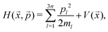
Proton-transfer reactions are vital in interstellar chemistry, and several charged species, such as H3+, HCO+, H3O+, and CH5+, act as efficient proton donors to neutral molecules found in the interstellar medium.1–8 The cross-sections or reaction rate coefficients for these proton-transfer processes are typically large because of the strong attractive interaction between charged and neutral molecules and the sizable proton affinity values of neutral interstellar species.9,10 In many of these proton-transfer reactions, the large excess energy is distributed into the protonated product molecule through the spectator stripping mechanism, where the transfer of a light proton particle occurs at large distances between the reactants, leading to a large initial vibrational energy in the H–X bond (X is a proton-accepting atom). An example is the H3+ + HCOOH → H2 + (HCOOH)H+ reaction,6–8,11 which is the focus of this study. The large excess energy in the protonated (HCOOH)H+ molecule can lead to its subsequent decomposition into two product channels: HCO+ + H2O and CO + H3O+. These product molecules, along with the parent HCOOH molecule, have been detected in the interstellar medium,12 making the corresponding [CO + H3O+]:[HCO+ + H2O] branching fraction an important parameter in astrochemical modeling. Additionally, the decomposition process associated with the unimolecular reaction of the energetic (HCOOH)H+ molecule can lead to a post-transition-state bifurcation (PTSB), where one transition-state (TS) structure results in two different product channels, as found in a previous theoretical study by Uggerud et al.8 They calculated the potential energy surface (PES) property using ab initio quantum chemistry and suggested that the initial protonated product takes the HC(OH)2+ structure, which subsequently isomerizes into the (HCO⋯H2O)+ type complex via the hydrogen transfer TS. This (HCO⋯H2O)+ complex can dissociate into both the HCO+ + H2O and CO + H3O+ fragments, but additional molecular rearrangements are required to achieve the latter CO + H3O+ fragments. The primary objective of this study is to computationally understand the dynamic mechanism of product branching in the dissociation of the (HCOOH)H+ molecule. As suggested by Uggerud et al.,8 we have investigated the indirect dissociation mechanism of the (HCO⋯H2O)+ type complex via the hydrogen transfer TS under the condition which the large excess energy generated by the protonation is redistributed as the internal energy. The energies which are more than the barrier height of the TS have been regarded as the thermal energies in this study. Notice that the proton affinities of the formic acid and H2 are 742.0 kJ mol−1 (177.3 kcal mol−1) and 4.39 eV (101.3 kcal mol−1), respectively.13,14 It is expected that there is enough energy to exceed the barrier in the (HCOOH)H+ molecule.
The TS typically connects one set of reactants with one set of products, resulting in a single reaction pathway as a function of the intrinsic reaction coordinate (IRC).15,16 However, there are also examples of chemical reactions where a single TS leads to multiple products.17–20 This phenomenon, known as PTSB,19,20 occurs due to the bifurcating nature of the post-transition-state reaction pathway on the PES. Notably in such cases, the product branching ratio is controlled by nuclear dynamics,21,22 although non-dynamical methods for practically estimating branching ratios have been proposed by several groups.23–28 In most of the previous PTSB studies, the product branching ratios were calculated using the well-known classical trajectory method initiated from the structures around the TS. More specifically, the quasi-classical trajectory (QCT) method, where quantized vibrational energies are also treated with a classical mechanics manner, is frequently employed. In fact, in the previous study by Uggerud et al.,8 on-the-fly ab initio QCT calculations were used to estimate the [CO + H3O+]:[HCO+ + H2O] branching fraction although only a small number of trajectories were integrated due to huge computational cost. In addition to this, it is worth mentioning that the QCT calculations frequently show zero-point leakage phenomenon leading to erroneous nuclear dynamics.29–31 Thus, the accuracy of the QCT scheme used in bifurcation reactions has not yet been fully understood. Motivated by this, we here calculate the branching fractions using three different nuclear dynamics methods including QCT, classical molecular dynamics (MD), and ring-polymer MD (RPMD)32–36 methods to understand the effect of the nuclear dynamics method in branching dynamics. Notice that the RPMD method can approximately describe both nuclear quantum effects and thermal fluctuation.29,37–53
In order to efficiently apply the above-mentioned three nuclear dynamics methods to the dissociation of (HCOOH)H+ into CO + H3O+ or HCO+ + H2O, we here utilize two different machine-learning (ML) computational techniques. One is the Δ-ML method54–56 for constructing a global PES. Generally, the electronic structure calculations considering the electronic correlation term for the systems, which have the large number of nuclear degrees of freedom and include heavy atoms, need high computational cost. Δ-ML method has been developed to avoid the expensive calculation cost with maintaining the accuracy of the PES. The low-level calculations such as Hartree-Fock and semiempirical methods are supposed as the fundamental PES, and the several high-level potential energies (and their gradients) are used as the correction term. The differences between the low-level and high-level PESs are utilized as the training data set. Then, the differential potential function Δ is evaluated using machine-learning technique. As will be described below, one can efficiently calculate both the potential energy and gradient values at a given nuclear structure using the PES of the protonated formic acid developed by the Δ-ML method.56 Thus, one can integrate a large number of trajectories. The second technique is a supervised ML classification approach, which is used to understand the detailed branching dynamics, i.e., the correlation between the initial conditions and the product branching. The branching fractions can be investigated through the ML analysis using statistical data such as the Cartesian coordinates and momenta or normal mode phase information at the initial TS region. It should be mentioned that, as the number of nuclear degrees of freedom in the chemical system increases, it can become difficult to identify which initial coordinates or momentum properties are important for the determination of the branching process. The ML classification approach helps us to identify the significant properties that dominate the bifurcation dynamics without relying on human intuition.57 Similar ML analysis techniques have been applied to other chemical reaction systems that exhibit PTSB.58–60 The details of the Δ-ML method, the MD method and those of the supervised ML algorithm are described in Section 2. The results of the dynamics and machine-learning analysis are discussed in Section 3. The conclusion is presented in Section 4.
2 Methodology
2.1 Development of Δ-ML PES
To integrate a statistically convergent number of MD trajectories within a reasonable computational timeframe, it is crucial to develop an accurate PES function. In this work, we have chosen to use the Δ-ML approach.56 This approach describes the final PES as the sum of a low-level PES function and a correction function, which are both functions of nuclear coordinates. In the Δ-ML approach developed by Bowman et al., these two functions are fitted using permutationally invariant polynomials to the results of ab initio calculations.61,62 In this work, we have chosen to use the semiempirical GFN2-xTB method63–65 as the low-level PES to avoid the time-consuming PES fitting procedure. The correction term was determined by fitting a dataset consisting of energy differences between the GFN2-xTB and ab initio calculations to a 3rd-order permutationally invariant polynomial function.
The ab initio level chosen in this study is the MP2 method with a 6-31G(d) basis set, as it allows for the qualitative comparison of the present results with those of previous studies by Uggerud et al.8 In order to develop the PES to describe the (HCOOH)H+ dissociation dynamics, a dataset of 192![[thin space (1/6-em)]](https://www.rsc.org/images/entities/char_2009.gif) 000 data points was generated by performing on-the-fly MD calculations at the MP2/6-31G(d) level. Subsequently, GFN2-xTB calculations were performed to obtain a dataset for fitting. The root-mean-square error (RMSE) for the fit was 209.9 cm−1. The fitting error for the correction energy is presented in Fig. S1 in the ESI.† All MP2/6-31G(d) level calculations were conducted using the Gaussian09 program package,66 while the GFN2-xTB calculations were performed using the xtb program (ver. 6.5.1),65,67 with an electronic temperature of 2500 K to achieve better convergence in the self-consistent charge iteration.64
000 data points was generated by performing on-the-fly MD calculations at the MP2/6-31G(d) level. Subsequently, GFN2-xTB calculations were performed to obtain a dataset for fitting. The root-mean-square error (RMSE) for the fit was 209.9 cm−1. The fitting error for the correction energy is presented in Fig. S1 in the ESI.† All MP2/6-31G(d) level calculations were conducted using the Gaussian09 program package,66 while the GFN2-xTB calculations were performed using the xtb program (ver. 6.5.1),65,67 with an electronic temperature of 2500 K to achieve better convergence in the self-consistent charge iteration.64
2.2 Three types of the real-time MD simulations
In this study, three types of MD simulations, which are the QCT, classical MD and RPMD, have been performed on the Δ-ML PES. To clarify the (HCOOH)H+ dissociation processes, all MD simulations started around the TS. Under the assumption that (HCOOH)H+ is thermalized and has the internal energies more than the potential energy at the TS, the energies over the TS barrier height were considered as the thermal energies. In this work, the temperatures 298, 1000, 2000 and 4000 K, which correspond to the thermal energies 0.6, 2.0, 4.0 and 8.0 kcal mol−1, were employed. For QCT, the initial coordinates and momenta were randomly sampled, considering the zero-point energy (ZPE) and thermal energy for each normal mode at the TS structure. On the other hand, for the RPMD and classical MD, the initial coordinates and momenta were sampled by path-integral molecular dynamics (PIMD) technique. Then, the real-time RPMD and classical MD simulations from the initial conditions obtained by the PIMD simulation were performed. The details of the QCT, PIMD, RPMD and classical MD are mentioned below.
2.2.1 QCT.
To evaluate the dynamics of the protonated formic acid dissociation, QCT simulations were performed using the Born–Oppenheimer molecular dynamics (BOMD) approach.68 The BOMD method, which is a tool in the Gaussian 09 program package, was used to solve the equations of motion (EOMs) by incorporating a Hessian-based integrator with a fifth-order polynomial fit. The simulations were run for approximately 500 fs, using the GFN2-xTB method with the Δ-ML PES. The initial coordinates and velocities were randomly sampled, considering the ZPE and thermal energy for each normal mode at the TS structure. The velocities for the imaginary frequency mode were sampled according to the statistical Boltzmann distribution, and the initial coordinates of the imaginary mode were always located on the TS.
2.2.2 PIMD.
To perform the real-time dynamics simulations, the PIMD simulations (based on the imaginary time path integral theory) were conducted to obtain the phase information of the thermal distribution at temperatures of 298, 1000, 2000, and 4000 K. The thermal phase distribution was used as the initial conditions for real-time dynamics simulations. The PIMD simulations were performed at the TS for each normal mode, including one imaginary mode, among the 12 modes. To maintain the molecular structures around the TS, the vibrational normal mode coordinates were employed instead of Cartesian coordinates.
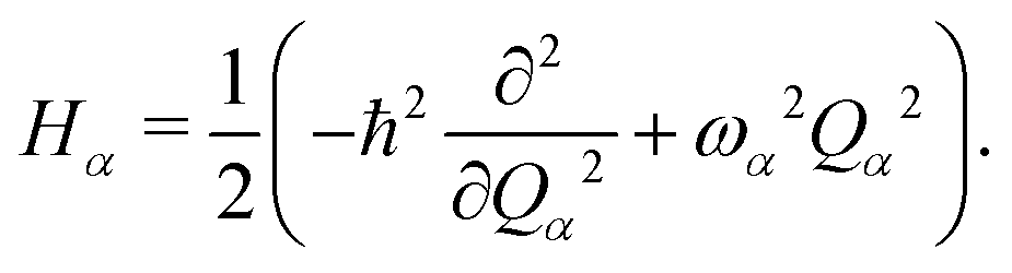
The PIMD simulations were carried out for a simple one-dimensional PES, V(Qα), in atomic units, where Qα is the α-th normal mode coordinate for the vibrational frequency at the stationary point. The quantum partition function Z at temperature T in the path integral representation is
| |  | (1) |
where
N is the number of beads,
β ≡ 1/
kBT represents a reciprocal temperature with the Boltzmann constant
kB,
ħ = 1 and
μ = 1 (in atomic units) are the reduced Planck constant and the reduced mass for the
Qα respectively, and
Qα = (
Q1α, ⋯,
QNα)
T is the
N-dimensional vector coordinate. The effective potential
Veff is given by
| | 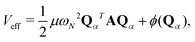 | (2) |
with

being a harmonic chain frequency and
A being a matrix whose the elements are described as
Aij = 2
δij −
δi,j+1 −
δi,j−1 with the cycle boundary conditions 0 →
N and
N + 1 → 1. The first term of the right-hand side of
eqn (2) represents the harmonic interaction between the adjacent beads. The second term is the bead-averaged physical potential
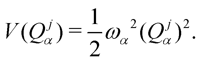
| |  | (3) |
where
V(
Qjα) is the harmonic potential with the
α-th vibrational frequency
ωα, and
| |  | (4) |
For imaginary frequency mode, where
ωα2 is negative, the
V(
Qjα) becomes
| |  | (5) |
with
f = 0.1 being the bias factor. In this study, the first term in
Veff has been diagonalized in the same manner as in previous studies.
69,70 The diagonalization of the matrix
NA is defined by
with the analytical diagonal eigenvalue matrix
Λ and the eigenvector
U. The eigenvalue matrix elements are represented by
| |  | (7) |
with
λ1 = 0 and
λN = 4
N. The eigenvector matrix elements are expressed as
| | 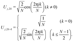 | (8) |
The coordinate
Qα can be transformed to
![[Q with combining tilde]](https://www.rsc.org/images/entities/b_char_0051_0303.gif) α
α using the eigenvector,
| |  | (9) |
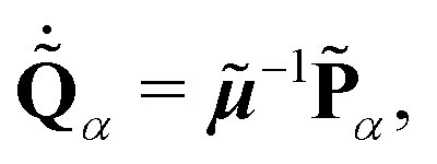
Using the newly defined coordinate
α and its conjugated momentum
![[P with combining tilde]](https://www.rsc.org/images/entities/b_char_0050_0303.gif) α
α = (
![[P with combining tilde]](https://www.rsc.org/images/entities/i_char_0050_0303.gif) 1α
1α,⋯,
Nα)
T, the Hamiltonian
H of the classical representation is defined as
| |  | (10) |
where
![[small mu, Greek, tilde]](https://www.rsc.org/images/entities/b_i_char_e0e0.gif)
is a diagonal matrix, whose elements are the fictitious mass for the newly defined phase space (
α,
α). The diagonal terms diag(
) = (
μ,
![[small mu, Greek, tilde]](https://www.rsc.org/images/entities/i_char_e0e0.gif) 2
2,⋯,
N) are expressed as
| | | j=1 = μ = 1, j = λjμ (2 ≤ j ≤ N). | (11) |
Note that the matrix
is constant for any vibrational mode when the number of beads
N is the same for all vibrational modes. The canonical equations of motion (EOMs) are then conventionally derived from
eqn (10):
| |  | (12) |
| | 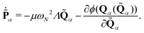 | (13) |
The EOMs were integrated by employing the velocity Verlet algorithm
71 with time step Δ
t = 0.20 fs with the Nóse–Hoover chain thermostat
72–74 for each vibrational mode. The initial phase information
α and
α were randomly chosen. The canonical ensemble was maintained until the expectation value of the internal energy converged – with a total of 11 × 10
6 steps. Note that the initial coordinates and momenta for the real-time dynamics for RPMD as well as classical MD were picked up from the ones every 1000 steps after the 1 × 10
6 steps simulations. The number of beads
N were set as 32, 10, 6, and 4 for the temperature
T = 298, 1000, 2000, and 4000 K. The EOMs were solved individually for all vibrational modes,
α ∈ (1, ⋯, 3
n − 6) (for nonlinear molecule), where
n is the number of atoms. The coordinates and their velocities

were transformed to (
Qα,
![[Q with combining dot above]](https://www.rsc.org/images/entities/b_char_0051_0307.gif) α
α)
via the inverse transformation of
eqn (9).
Once the phase information for all vibrational modes was gathered, the vibrational normal mode can then be transformed conventionally to Cartesian coordinates and their time derivatives:
| |  | (14) |
where
![[q with combining right harpoon above (vector)]](https://www.rsc.org/images/entities/i_char_0071_20d1.gif) j
j = (
qj1, ⋯,
qj3n)
T and
![[Q with combining right harpoon above (vector)]](https://www.rsc.org/images/entities/i_char_0051_20d1.gif) j
j = (
Qj1, ⋯,
Qjα+6, ⋯,
Qj3n)
T are the mass-weighted Cartesian coordinate vector and the normal mode coordinate vector for
j-th bead, respectively. Notice that (
Q1, ⋯,
Q6) represents the translational and rotational (not vibrational) modes.

is the 3
n × 3
n unitary matrix used to obtain the vibrational frequency diagonal matrix,
Ω, diag(
Ω) = (
ω12, ⋯,
ωα+62, ⋯,
ω3n2). The Cartesian coordinates

and their velocities for
j-th bead can eventually be obtained by
| |  | (15) |
where Δ
![[x with combining right harpoon above (vector)]](https://www.rsc.org/images/entities/i_char_0078_20d1.gif) j
j is the displacement coordinates:
with

being the 3
n-dimensional Cartesian coordinate vector at the stationary point where is the TS in this study.

is the diagonal matrix whose elements
ml correspond to the atomic mass for the
l-th Cartesian coordinate. Note that the centroid of beads is written by
| |  | (17) |
Likewise, their velocities can be obtained based on
eqn (14), (15) and (17).
2.2.3 RPMD.
The semiclassical real-time MD simulation, referred to as the RPMD method,32–36 was carried out at temperature T = 298, 1000, 2000, and 4000 K. The RPMD method, which can represent nuclear quantum effects such as ZPE and quantum tunneling,37,38 has been extensively used.29,39–53 In contrast with the Hamiltonian for one-dimensional normal mode of PIMD, the Hamiltonian for RPMD is defined for the (3n × N bead)-multidimensional system from Cartesian coordinate representation:| | 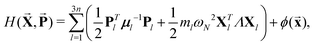 | (18) |
where Xl = (X1l, ⋯,XNl)T and Pl = (P1l, ⋯,PNl)T are the newly defined N-dimensional coordinate and its conjugated momentum vectors, respectively. The Xl were obtained from the N-dimensional l-th Cartesian coordinate vector xl = (x1l, ⋯,xNl)T:| |  | (19) |
![[X with combining right harpoon above (vector)]](https://www.rsc.org/images/entities/b_char_0058_20d1.gif) ,
, ![[P with combining right harpoon above (vector)]](https://www.rsc.org/images/entities/b_char_0050_20d1.gif) and
and ![[x with combining right harpoon above (vector)]](https://www.rsc.org/images/entities/b_char_0078_20d1.gif) are the (3n × N bead)-dimensional newly defined coordinates = (XT1, ⋯, XT3n), their conjugated momenta = (PT1, ⋯, PT3n), and the Cartesian coordinates = (xT1, ⋯, xT3n), respectively. The fictitious mass matrix for μl for (Xl,Pl) has the diagonal elements of the atomic mass of the l-th Cartesian coordinate:The last term of eqn (18) is the average physical potential:
are the (3n × N bead)-dimensional newly defined coordinates = (XT1, ⋯, XT3n), their conjugated momenta = (PT1, ⋯, PT3n), and the Cartesian coordinates = (xT1, ⋯, xT3n), respectively. The fictitious mass matrix for μl for (Xl,Pl) has the diagonal elements of the atomic mass of the l-th Cartesian coordinate:The last term of eqn (18) is the average physical potential:| |  | (21) |
where V is the physical potential energy.
The EOMs of eqn (18) were then calculated by the velocity Verlet algorithm71 with time step Δt = 0.50 fs for the real-time propagation without the thermostat. The total simulation time was 500 fs, which was the same as that for the classical MD simulation described below. The RPMD and subsequent classical MD simulations for the real-time dynamics were performed using the PIMD program (ver. 2.4.0) developed by Shiga.75
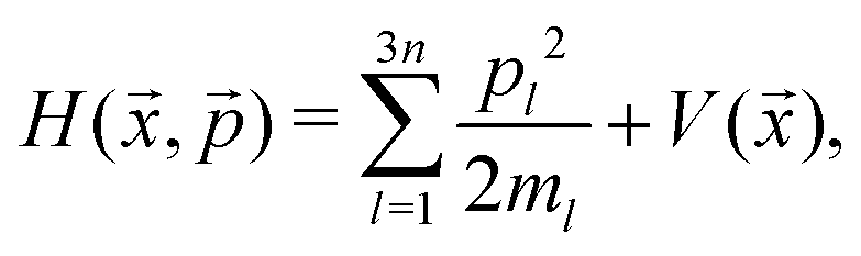
2.2.4 Classical MD.
Thermalization has been discussed in the PIMD section, and the real-time dynamics has been explained in the RPMD section. In the classical MD simulations, the number of beads N was set to 1. In this case, the Hamiltonian of eqn (10) has been re-expressed for thermalization as| |  | (22) |
Note that the expectation value of the internal energy for this thermalization lacks the contribution of the ZPE.
The Hamiltonian (without the thermostat) for the real-time dynamics therefore becomes the conventional classical Hamiltonian:
| |  | (23) |
where
and
![[p with combining right harpoon above (vector)]](https://www.rsc.org/images/entities/i_char_0070_20d1.gif)
are the Cartesian coordinates
= (
x1, ⋯,
x3n)
T and the conjugated momenta
= (
p1, ⋯,
p3n)
T, respectively.
2.3 Supervised ML
Supervised ML was performed to analyze the features dictating the branching reaction. In this study, binary classifications of the branching dynamics were carried out based on 108 TS features, including vibrational modes, their velocities, bond distances, bond angles, and dihedral angle. The random forest (RF), K-nearest neighbor (KNN), multi-layer perceptron (MLP), stochastic gradient descent (SGD), support vector machine (SVM), and logistic regression (LogR) algorithms, which are implemented in the Scikit-Learn Python Library, were employed in this study. The lightGBM (LGB) algorithm implemented in Python3 was also carried out. Both of RF and LGB classifiers are decision tree-based algorithms. The RF is the method based on the bagging also known as bootstrap aggregating that is a parallel ensemble learning method, whereas boosting algorithm used in the LGB method is a sequential ensemble learning method. The SelectFromModel method with the RF model of the Scikit-learn library was used to perform feature selection and reduction to half in order to improve the classification accuracy score. The accuracy of each classification model was obtained by performing a 5-fold cross validation on the most relevant 54 TS features. To obtain the accuracy scores with eliminating the dimension influences of each feature,57 the data sets were normalized into [0, 1]. An optimized RF (RF Opt) and LGB models were obtained by performing hyperparameter optimization using the GridSearchCV method of the Scikit-learn library in Python3. The data sets were initially split as the training and validation data (75%) and test data (25%), then hyperparameter optimization was performed with 5-fold cross validation in the training and validation data. The parameters which are the number of estimator, criterion, max_depth, and max_features, were optimized for the RF model. In contrast, the minimum number of data per leaf, the number of leaves, the number of iterations, the coefficients of L1 and L2 regularization, and metric were tuned for the LGB method with gradient boosting decision tree (GBDT). The learning rate was set to 0.05 for the LGB model to avoid overfitting. Eventually the RF Opt and LGB models with best estimators were generated for the training and validation data. Once the high accuracy score for the test data using the RF Opt and LGB models are obtained, we can extract the reliable feature importance of the RF and LGB models. Notice that the gain-based feature importance for LGB model was obtained in this study.
3 Results and discussion
3.1 Potential energy profile
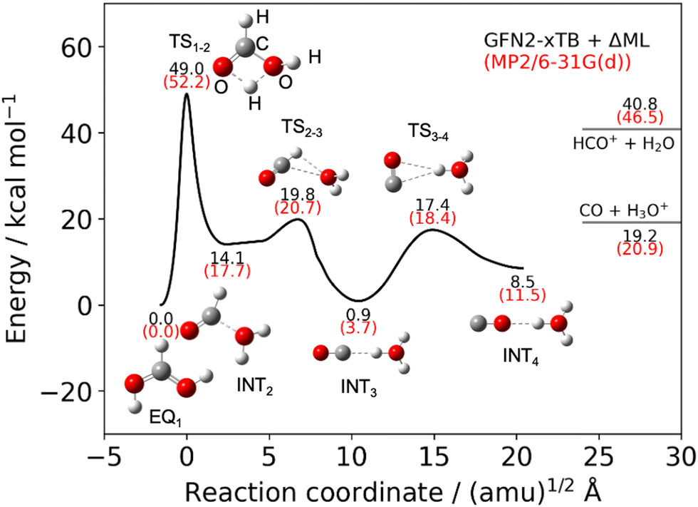
Fig. 1 illustrates the reaction pathway (represented by a black line) from the reactant (EQ1), which is the equilibrium protonated formic acid, to the complex intermediate CO⋯H3O+ (INT4), and includes key geometries. As previously discussed in the methodology section, the PES was calculated using the GFN2-xTB approach with correction by the Δ-ML method, with the reactant set at 0.00 kcal mol−1. The potential energy curve is composed of three IRC calculations and is condensed into a single curve. The first TS, denoted as TS1–2, connects EQ1 and INT2 and describes the large energy barrier in the proton/hydrogen transfer reaction between two oxygen atoms. However, it is expected that the reaction can overcome this barrier because the protonated formic acid has large excess energy.6–8,11 Beyond TS1–2, the potential energies of the remaining intermediates and TSs are lower than the TS1–2 energy. INT2 and TS2–3 have precursor structures of the HCO+ + H2O product. Then, the proton-transfer reaction OCH+⋯H2O → OC⋯H3O+ occurs from TS2–3 to INT3. The CO molecule rotates between INT3 and INT4 through TS3–4. The potential energies written in black and red correspond to the values obtained from our PES and MP2/6-31G(d) level calculations, respectively. Additionally, the values are compared with results from previous theoretical studies that were calculated using the MP2/6-31G(d) level.8 Our potential profiles are in good agreement with the previous study (see Table S1, ESI†). The quality of the PES is sufficient for performing appropriate MD simulations, as the protonated formic acid has excess energy. In this study, it is not important for the molecule to tunnel through the barrier in the reaction pathway. The potential energy values are listed in Table S1 in the ESI.†
 |
| | Fig. 1 Potential energy curve calculated using GFN2-xTB method with the Δ-ML approach for the dissociation reactions, illustrating key geometries. The potential energies of the key geometries are compared with MP2/6-31G(d). | |
3.2 PIMD sampling
The coordinates and momenta at TS1–2 were sampled on the PES (described by eqn (4) and (5)) by the PIMD technique to perform the RPMD method, which is the real-time dynamics simulation. Fig. S2 and S3 in the ESI,† show the imaginary vibrational frequency mode and the temperature-dependent populations of vibrational states of harmonic oscillators with different wavenumbers ![[small nu, Greek, tilde]](https://www.rsc.org/images/entities/i_char_e0e1.gif) α = ωα/2πc, where c is the speed of light. The formula of the population is expressed as eqn (A8) in Appendix A. As shown in Fig. S3 (ESI†), higher excitation occurs as temperature increases and the vibrational frequency is smaller as expected. At 4000 K, for the smallest wavenumber 2, the vibrational mode is populated even in the 20-th excited state. In contrast, vibrational excitation over the 4-th excited state rarely occurs for the largest frequency mode 12, even at 4000 K.
α = ωα/2πc, where c is the speed of light. The formula of the population is expressed as eqn (A8) in Appendix A. As shown in Fig. S3 (ESI†), higher excitation occurs as temperature increases and the vibrational frequency is smaller as expected. At 4000 K, for the smallest wavenumber 2, the vibrational mode is populated even in the 20-th excited state. In contrast, vibrational excitation over the 4-th excited state rarely occurs for the largest frequency mode 12, even at 4000 K.
Fig. S4 in the ESI,† illustrates the expectation value of the configuration space for the Q2 and Q12 modes, corresponding to the smallest and largest frequencies, respectively. The results of thermalization by the PIMD and classical procedures are depicted in Fig. S4a–d (ESI†). The black line represents the magnitude of the zero-point vibrational wave function |Ψ0|2. In the case of the smallest frequency mode shown in Fig. S4a and c (ESI†), the expectation values from both PIMD and classical simulations at temperatures of 1000, 2000 and 4000 K are similar, as the ZPE is smaller than the expectation value of the internal energy 〈E〉 (as seen in Table S2 in the ESI†); thus, quantum effects are not significant at higher temperatures. At 298 K, the distribution of coordinates is along the line of |Ψ0|2 in Fig. S4a and c (ESI†). Conversely, in Fig. S4b (ESI†), the expectation values of the configuration space at 298, 1000, and 2000 K obtained using PIMD sampling are distributed along the zero-point vibrational wave function |Ψ0|2. At 4000 K, the coordinate distribution has a larger tail than |Ψ0|2. In contrast with PIMD sampling, the distributions at temperatures below 2000 K obtained using classical sampling in Fig. S4d (ESI†) are narrower than |Ψ0|2 because the configuration space has a classical limit. The distributions at 4000 K shown in Fig. S4b and d (ESI†) are similar, as the internal energy is dominated by kBT rather than ZPE at this temperature.
Table S2 (ESI†) presents the expectation value of the internal energies 〈E〉 obtained using PIMD sampling and the analytical internal energy 〈Uq〉 for the quantum harmonic oscillator at various temperatures, including the ZPE. It is observed that the energy calculated using PIMD simulations 〈E〉 for all normal modes at each temperature is in good agreement with the analytical value 〈Uq〉 (as described in eqn (A7) in Appendix A). At 298 K, ZPE dominates the 〈E〉. As the temperature increases, kBT becomes more dominant over ZPE, particularly for smaller wavenumber α. In contrast, Table S3 (ESI†) illustrates the expectation values of the internal energies 〈E〉 obtained using classical sampling and the analytical values 〈Uc〉 (as described in eqn (A3) in Appendix A). The 〈Uc〉 is only temperature-dependent and does not depend on the vibrational frequencies. As a result, the energy 〈E〉 for the classical procedure for all normal modes is almost the same at each temperature. From these results, it can be concluded that both thermalizations via PIMD and classical procedures are effective.
3.3 Branching fraction
Fig. 2 illustrates the branching fraction between [CO + H3O+] and [HCO+ + H2O] from QCT, classical MD, and RPMD simulations at various temperatures. The number of trajectories correlated with the branching and the total number of trajectories are listed in Table 1. At 298 K, the CO + H3O+ fragments are dominant in all simulations shown in Fig. 2. As the temperature increases, the HCO+ + H2O branching fraction increases. The fraction behavior for QCT is significantly different from that of other simulations. The HCO+ + H2O becomes the primary product at 4000 K for QCT, while the main products for classical MD and RPMD simulations remain CO + H3O+. This property is likely influenced by the ZPE leakage,29–31 which is frequently discussed as the problem for the QCTs51–53,60,76,77 which have excessive energies (vibrational quantization energies in classical trajectories). It can be predicted that the ZPE leakage phenomenon substantially influences the branching dynamics. Recently, Tremblay et al. have also shown that the ZPE percentage affects the bifurcation ratio.78 The HCO+ + H2O fragments for RPMD are slightly less than those for classical MD, but both tendencies are similar. One possible reason of the slight difference at high temperature could be the procedure for solving the EOMs. For RPMD, the EOMs for the each bead were solved then the centroid get influenced by the mean force from the beads. In contrast, the classical MD were time-propagated based on the solution of the EOMs of the classical nuclei. As shown in Fig. S4 (ESI†), the initial configuration distribution at high temperature doesn't really contribute the difference of the branching fractions between the RPMD and classical MD because the configuration distribution at high temperature for both classical MD and RPMD are quite similar. Table 2 shows the comparison the branching fractions from three types of simulations with previous studies. The previous theoretical study8 shows that the HCO+ + H2O branching fraction increases as temperature increases, which indicates our simulations are qualitatively agreement with the previous one. The product ratios of HCO+ + H2O fragments measured at 298 and 353 K were 30%6 and 17.8%.11 Both values are relatively larger than our data for all simulations at 298 K. From the results, it could be tentatively estimated that the direct dissociation process right after the protonation contributes the increasing of the HCO+ + H2O products because our simulations have considered the indirect dissociation process after the excess energy from the proton affinity are thermalized as the internal energy, which is also knows as the intramolecular vibrational redistribution. In the following section, we discuss the crucial initial phase information at TS1–2, which has a huge effect on the bifurcation dynamics, using ML analysis.
 |
| | Fig. 2 Branching fraction profiles as a function of temperature for (a) QCT, (b) classical MD, and (c) RPMD. The black and red lines represent the product ratio of the HCO+ + H2O and CO + H3O+, respectively. | |
Table 1 Number of HCO+ + H2O and CO + H3O+ fragment trajectories, and the total number of trajectories NTraj. at each temperature for QCT, classical MD and RPMD simulations
|
T/K |
HCO+ + H2O |
CO + H3O+ |
N
Traj.
|
| QCT |
| 298 |
272 |
2793 |
3065 |
| 1000 |
531 |
1535 |
2066 |
| 2000 |
1016 |
1188 |
2204 |
| 4000 |
1249 |
984 |
2233 |
| Classical MD |
| 298 |
83 |
2693 |
2776 |
| 1000 |
390 |
1877 |
2267 |
| 2000 |
524 |
1705 |
2229 |
| 4000 |
572 |
1147 |
1719 |
| RPMD |
| 298 |
4 |
2212 |
2216 |
| 1000 |
201 |
2359 |
2560 |
| 2000 |
280 |
1740 |
2020 |
| 4000 |
492 |
1418 |
1910 |
Table 2 Branching fractions with the standard deviations of HCO+ + H2O and CO + H3O+ products at each temperature for QCT, classical MD and RPMD simulations compared with previous studies
|
T/K |
Products/% |
| HCO+ + H2O |
CO + H3O+ |
| QCT |
| 298 |
8.9 ± 0.5 |
91.1 ± 0.5 |
| 1000 |
25.7 ± 1.0 |
74.3 ± 1.0 |
| 2000 |
46.1 ± 1.1 |
53.9 ± 1.1 |
| 4000 |
55.9 ± 1.1 |
44.1 ± 1.1 |
| Classical MD |
| 298 |
3.0 ± 0.3 |
97.0 ± 0.3 |
| 1000 |
17.2 ± 0.8 |
82.8 ± 0.8 |
| 2000 |
23.5 ± 0.9 |
76.5 ± 0.9 |
| 4000 |
33.3 ± 1.1 |
66.7 ± 1.1 |
| RPMD |
| 298 |
0.2 ± 0.1 |
99.8 ± 0.1 |
| 1000 |
7.9 ± 0.5 |
92.1 ± 0.5 |
| 2000 |
13.9 ± 0.8 |
86.1 ± 0.8 |
| 4000 |
25.8 ± 1.0 |
74.2 ± 1.0 |
| Theo. (ref. 8) |
| 298 |
40 |
60 |
| 1000 |
60 |
40 |
| Exp. (ref. 6) |
| 298 |
30 |
70 |
| Exp. (ref. 11) |
| 353 |
17.8 |
82.2 |
3.4 Binary classification by the supervised ML algorithms
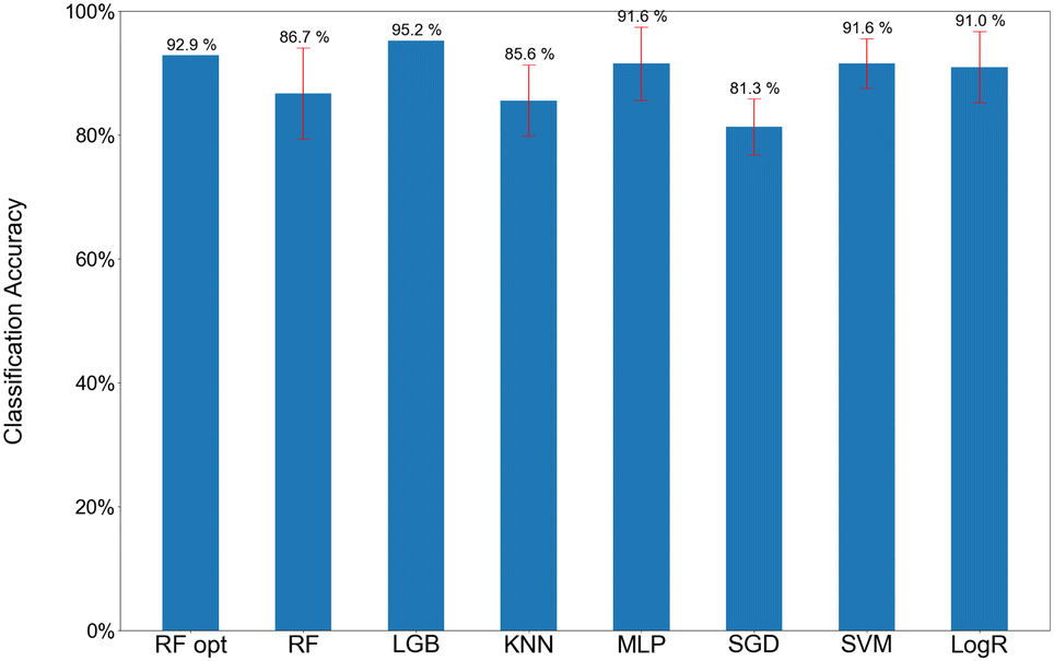
Fig. 3 illustrates the accuracy scores for the 54 TS features in the binary classification of the CO + H3O+ and HCO+ + H2O dissociation trajectories at 298 K for the classical MD simulations using various classification models. Note that an equal number of CO + H3O+ and HCO+ + H2O dissociation trajectories were included in the data set for the ML analysis. As mentioned above, the data sets were normalized into [0, 1] to adjust the magnitude and to eliminate the dimension effects of each feature. The scores and error bars represent the means and standard deviations for a 5-fold cross validation, respectively. The RF model provided an accuracy of 86.7%, which was improved to 92.9%, using the RF Opt model. The accuracy score of the LGB algorithm was 95.2% which was a best score in the algorithms. Other models such as KNN, MLP, SGD, SVM, and LogR also had excellent performance, with accuracy ranging from 81.3–91.6%.
 |
| | Fig. 3 Accuracy scores in the binary classification for the 298 K classical simulation. | |
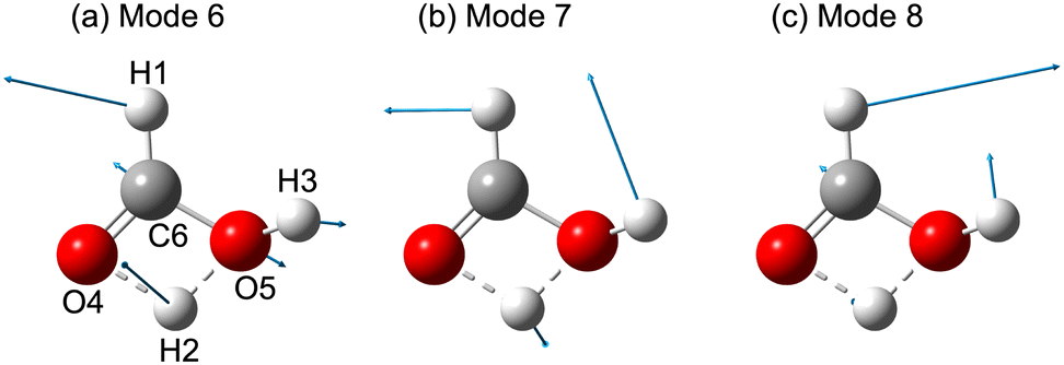
The relative importance of various 54 TS features to the RF Opt and LGB models, such as the total energy for the initial coordinates and momenta, the velocity between the center of mass of HCO+ and H2O, bond lengths, bond angles, dihedral angles, mass-weighted displacement (MWD), and velocity (MWV) for each normal mode, are shown in Fig. 4a and b. The numbers in parentheses for each feature represent the numbered atoms: H1, H2, H3, O4, O5, and C6 (see Fig. 5a). Fig. 4 was constructed based on the data set having 83 dissociation trajectories of each CO + H3O+ and HCO+ + H2O dissociation. Note that Fig. S5 and S6 (ESI†) present comparable accuracy scores and feature importance distributions composed from three different subsets of the data which are 60, and 40 of each dissociation channel. This indicates that the number of trajectories was sufficient to generate a reliable result. Both of Fig. 4a and b derived from the RF and LGB models, which have 92.9% and 95.2% accuracy scores, show the similar representative significant features. Notice that these scores are the test scores not training scores, which indicates that the models have avoided overfitting. The angle ∠(H1–O5–O4) is presented as the most important feature. The motion of H1, which possesses the lightest weight among H1, O5, and O4, is important for the bifurcation reaction. In Fig. 4, the importance to the MWDs of modes 6 and 7, and to the MWV of mode 8, also demonstrate the significant features in the classification. The normal mode vectors for modes 6, 7, and 8 (shown in Fig. 5) consist of a considerable H1 motion contribution. The bond distance between O5 and C6, and the velocity between the center of mass of HCO+ and H2O, ![[v with combining right harpoon above (vector)]](https://www.rsc.org/images/entities/i_char_0076_20d1.gif) HCO+–H2O, are also important features in the classification, as shown in Fig. 4. Fig. S7 (ESI†) displays the accuracy scores for the most relevant six features for each algorithm. The high accuracy scores suggest that these six features are important in the binary classification. In this case, most representative features were also the ∠(H1–O5–O4) for both of RF and LGB models. At 4000 K, significant features (as seen in Fig. S8 in the ESI†) are not present in the dynamics, indicating that it is difficult to classify the trajectories at this temperature. This suggests that interactions between vibrational modes occur efficiently during the branching process at higher temperatures.
HCO+–H2O, are also important features in the classification, as shown in Fig. 4. Fig. S7 (ESI†) displays the accuracy scores for the most relevant six features for each algorithm. The high accuracy scores suggest that these six features are important in the binary classification. In this case, most representative features were also the ∠(H1–O5–O4) for both of RF and LGB models. At 4000 K, significant features (as seen in Fig. S8 in the ESI†) are not present in the dynamics, indicating that it is difficult to classify the trajectories at this temperature. This suggests that interactions between vibrational modes occur efficiently during the branching process at higher temperatures.
 |
| | Fig. 4 Importance of 54 TS features with respect to the 298 K classical simulation derived from the (a) RF Opt and (b) LGB models. | |
 |
| | Fig. 5 Normal mode vectors at the TS1–2 for (a) mode 6, Q6 with the atom numbering, (b) mode 7, Q7, and (c) mode 8, Q8. | |
3.5 Significant features for the bifurcation reaction
Fig. 6 shows the normalized distribution of the most relevant six features of the CO + H3O+ and HCO+ + H2O dissociation trajectories for the 298 K classical MD simulation. As shown in Fig. 6a, the initial configurations with wider and narrower angles of ∠(H1–O5–O4) contribute to dissociation into HCO+ + H2O and CO + H3O+, respectively. The large velocity of mode 8, which is correlated with the opening motion of ∠(H1–O5–O4), also represents dissociation into HCO+ + H2O, as shown in Fig. 6b. Fig. 6c and d show that negative displacement of modes 6 and 7 (see Fig. 5) contributes to HCO+ + H2O dissociation. The negative vector directions of modes 6 and 7 are consistent with the positive direction of mode 8. The results suggest that structures of HCO+ that are almost linear play a role in the HCO+ + H2O dissociation process, despite the H1 atom getting close to H2O. This is a counter-intuitive bifurcation process that can be revealed through ML analysis without human intuition. Fig. 6 shows the normalized distribution as a function of the data set for the most relevant six features of the CO + H3O+ and HCO+ + H2O dissociation trajectories for the 298 K classical MD simulation. In Fig. 6e, the data shows that the initial configuration with a shrinking O5–C6 bond distance is important for the dissociation into the HCO+ + H2O fragment. This suggests that the repulsive potential energy of the O5–C6 bond plays a role in guiding the trajectories toward a higher potential energy than the HCO+ + H2O dissociation channel. Fig. 6f shows the velocity distribution of HCO+–H2O. Both the HCO+ + H2O and CO + H3O+ dissociation have stretching velocities, but the lower stretching velocities dissociate to the HCO+ + H2O instead of the higher velocities. This is also a counter-intuitive branching. The results indicate the large HCO+–H2O velocity at t = 0 fs is insignificant to the HCO+ + H2O dissociation process. All Fig. 6a–f demonstrate feature overlap, implying that the dissociation dynamics are not dependent only on a single mode.
 |
| | Fig. 6 Normalized distribution for the (a) H1–O5–O4 bond angle, (b) mass-weighted velocity for mode 8, (c) MWD for mode 6, (d) MWD for mode 7, (e) O5–C6 bond distance, and (f) velocity between the center of mass of HCO+ and H2O at the TS1–2. Red and blue bars represent the feature distribution with respect to the HCO+ + H2O and CO + H3O+ dissociation trajectories of the classical MD simulations at 298 K. | |
4 Conclusion
We investigated the dissociation processes of the (HCOOH)H+ molecule from the TS using three types of molecular dynamics simulations: QCT, classical MD, and RPMD at temperatures of 298, 1000, 2000, and 4000 K. The effects of temperature were considered in relation to the large excess energies from the proton affinity of (HCOOH)H+. The dissociation into HCO+ + H2O, which has a higher potential energy (40.8 kcal mol−1) than the CO + H3O+ dissociation channel (19.2 kcal mol−1), increases as the temperature increases. We found that the branching fractions of the QCT are significantly different from the fractions obtained in other classical MD and RPMD simulations. The initial coordinates and momenta used in the QCT include the excess energy necessary to describe the vibrational quantization in classical particles, but this ZPE leakage phenomenon leads to inaccurate branching. The HCO+ + H2O branching fractions obtained from the three types of simulations at 298 K were underestimated the experimental results. It could be provisionally evaluated that the direct dissociation process after the protonation contributes the product ratio. We will perform the development of more accurate PES to obtain a more quantitative branching fraction then report elsewhere the discussion.
We used ML analysis to determine which features at the TS strongly contribute to the HCO+ + H2O dissociation. Good results were obtained for the binary classification of the HCO+ + H2O and CO + H3O+ dissociation trajectories using the RF Opt, RF, LGB, KNN, MLP, SGD, SVM, and LogR algorithms in relation to 298 K classical simulations. The feature importance for the classical MD simulations at 298 K was determined by the RF Opt model. We found that the initial configuration of the linear HCO+ and O5–C6 shrinking, and the initial velocity of the stretching direction between the center of mass of HCO+ and H2O are significantly important for the HCO+ + H2O dissociation process. In this study, ML analysis proved vital for identifying bifurcation reaction selectivity from TS features.
Author contributions
TM and TT devised and supervised the project. TT acquired the funding. TM, SI, YH, and TT designed the methodology. TM, SI, YH, and YK performed the calculations. TM, SI, YH, and YK analyzed and visualized the data. TM, SI, YH, and TT verified the methods and the results. TM and TT wrote the original draft and edited and reviewed it.
Conflicts of interest
There are no conflicts to declare.
Appendix A. Canonical ensemble for one-dimensional harmonic oscillator
The one-dimensional classical Hamiltonian for harmonic oscillator of α th mode is expressed as eqn (22):| | 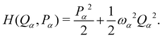 | (A1) |
The partition function Zc of a classical representation is defined as
| |  | (A2) |
where
h is Planck constant with the relation

. The internal energy 〈
Uc〉 therefore becomes
| |  | (A3) |
In contrast, the quantum expression of the Hamiltonian is written as
| |  | (A4) |
The well-known energy representation solved by the time-independent Schrödinger equation is
| |  | (A5) |
where
nvib is the vibrational quantum number. The partition function
Zq for the quantum harmonic oscillator is represented by
| |  | (A6) |
with some linear algebra. The temperature-dependent internal energy 〈
Uq〉 for the quantum representation is described as
| |  | (A7) |
The internal energy 〈
Uq〉 depends on temperature and the vibrational frequency while the energy 〈
Uc〉 is the only temperature-dependent parameter. The probability

of populating the state
nvib with energy

can be represented as
| |  | (A8) |
Acknowledgements
This work is supported by a grant from the Japan Society for the Promotion of Science (Grants-in-Aid for Scientific Research KAKENHI No. 20H05847).
Notes and references
- J. L. Neill, A. L. Steber, M. T. Muckle, D. P. Zaleski, V. Lattanzi, S. Spezzano, M. C. McCarthy, A. J. Remijan, D. N. Friedel, S. L. Widicus Weaver and B. H. Pate, J. Phys. Chem. A, 2011, 115, 6472–6480 CrossRef CAS PubMed.
- P. Ehrenfreund, L. d'Hendecourt, S. Charnley and R. Ruiterkamp, J. Geophys. Res.: Planets, 2001, 106, 33291–33301 CrossRef CAS.
- D. Smith, P. Spanel and T. J. Millar, Mon. Not. R. Astron. Soc., 1994, 266, 31–34 CrossRef CAS.
- D. A. Fairley, G. B. I. Scott, C. G. Freeman, R. G. A. R. Maclagan and M. J. McEwan, J. Chem. Soc., Faraday Trans., 1996, 92, 1305–1309 RSC.
- M. Ohishi, S.-i Ishikawa, T. Amano, H. Oka, W. M. Irvine, J. E. Dickens, L. M. Ziurys and A. J. Apponi, Astrophys. J., 1996, 471, L61–L64 CrossRef CAS PubMed.
- G. I. Mackay, A. C. Hopkinson and D. K. Bohme, J. Am. Chem. Soc., 1978, 100, 7460–7464 CrossRef CAS.
- G. I. Mackay, S. D. Tanner, A. C. Hopkinson and D. K. Bohme, Can. J. Chem., 1979, 57, 1518–1523 CrossRef CAS.
- O. Sekiguchi, V. Bakken and E. Uggerud, J. Am. Soc. Mass Spectrom., 2004, 15, 982–988 CrossRef CAS PubMed.
- S. G. Lias, J. F. Liebman and R. D. Levin, J. Phys. Chem. Ref. Data, 1984, 13, 695–808 CrossRef CAS.
- E. P. L. Hunter and S. G. Lias, J. Phys. Chem. Ref. Data, 1998, 27, 413–656 CrossRef CAS.
- S. E. Sanni, P. A. Alaba, E. Okoro, M. Emetere, B. Oni, O. Agboola and A. O. Ndubuisi, Sustainable Energy Technol. Assess., 2021, 45, 101078 CrossRef.
- E. Herbst, Annu. Rev. Phys. Chem., 1995, 46, 27–53 CrossRef CAS.
-
NIST Chemistry Webbook, https://www.nist.gov Search PubMed.
- T. Oka, Chem. Rev., 2013, 113, 8738–8761 CrossRef CAS PubMed.
- H. Eyring, J. Chem. Phys., 1935, 3, 107 CrossRef CAS.
- J. L. Bao and D. G. Truhlar, Chem. Soc. Rev., 2017, 46, 7548–7596 RSC.
- S. Maeda, Y. Harabuchi, Y. Ono, T. Taketsugu and K. Morokuma, Int. J. Quantum Chem., 2015, 115, 258–269 CrossRef CAS.
- J. Rehbein and B. K. Carpenter, Phys. Chem. Chem. Phys., 2011, 13, 20906–20922 RSC.
- D. H. Ess, S. E. Wheeler, R. G. Iafe, L. Xu, N. Çelebi-Ölçüm and K. N. Houk, Angew. Chem., Int. Ed., 2008, 47, 7592–7601 CrossRef CAS PubMed.
- S. R. Hare and D. J. Tantillo, Pure Appl. Chem., 2017, 89, 679–698 CrossRef CAS.
- S. Pratihar, X. Ma, Z. Homayoon, G. L. Barnes and W. L. Hase, J. Am. Chem. Soc., 2017, 139, 3570–3590 CrossRef CAS PubMed.
- Z. Yang and K. N. Houk, Chem. – Eur. J., 2018, 24, 3916–3924 CrossRef CAS.
- Z. Yang, X. Dong, Y. Yu, P. Yu, Y. Li, C. Jamieson and K. N. Houk, J. Am. Chem. Soc., 2018, 140, 3061–3067 CrossRef CAS PubMed.
- B. K. Carpenter, Annu. Rev. Phys. Chem., 2005, 56, 57–89 CrossRef CAS.
- T. H. Peterson and B. K. Carpenter, J. Am. Chem. Soc., 1992, 114, 766–767 CrossRef CAS.
- J. Zheng, E. Papajak and D. G. Truhlar, J. Am. Chem. Soc., 2009, 131, 15754–15760 CrossRef CAS PubMed.
- S. Lee and J. M. Goodman, J. Am. Chem. Soc., 2020, 142, 9210–9219 CrossRef CAS PubMed.
- S. Lee and J. M. Goodman, Org. Biomol. Chem., 2021, 19, 3940–3947 RSC.
- N. Bulut, A. Aguado, C. Sanz-Sanz and O. Roncero, J. Phys. Chem. A, 2019, 123, 8766–8775 CrossRef CAS PubMed.
- S. Habershon and D. E. Manolopoulos, J. Chem. Phys., 2009, 131, 244518 CrossRef PubMed.
- G. Czakó, A. L. Kaledin and J. M. Bowman, J. Chem. Phys., 2010, 132, 164103 CrossRef PubMed.
- I. R. Craig and D. E. Manolopoulos, J. Chem. Phys., 2004, 121, 3368–3373 CrossRef CAS PubMed.
- I. R. Craig and D. E. Manolopoulos, J. Chem. Phys., 2005, 122, 084106 CrossRef PubMed.
- I. R. Craig and D. E. Manolopoulos, J. Chem. Phys., 2005, 123, 034102 CrossRef PubMed.
- T. F. Miller III and D. E. Manolopoulos, J. Chem. Phys., 2005, 123, 154504 CrossRef PubMed.
- S. Habershon, D. E. Manolopoulos, T. E. Markland and T. F. Miller III, Annu. Rev. Phys. Chem., 2013, 64, 387–413 CrossRef CAS PubMed.
- R. Pérez De Tudela, F. J. Aoiz, Y. V. Suleimanov and D. E. Manolopoulos, J. Phys. Chem. Lett., 2012, 3, 493–497 CrossRef PubMed.
- R. Pérez De Tudela, Y. V. Suleimanov, J. O. Richardson, V. Sáez Rábanos, W. H. Green and F. J. Aoiz, J. Phys. Chem. Lett., 2014, 5, 4219–4224 CrossRef PubMed.
- Y. V. Suleimanov, R. Collepardo-Guevara and D. E. Manolopoulos, J. Chem. Phys., 2011, 134, 044131 CrossRef PubMed.
- Y. V. Suleimanov, J. Phys. Chem. C, 2012, 116, 11141–11153 CrossRef CAS.
- Y. V. Suleimanov, R. Pérez De Tudela, P. G. Jambrina, J. F. Castillo, V. Sáez-Rábanos, D. E. Manolopoulos and F. J. Aoiz, Phys. Chem. Chem. Phys., 2013, 15, 3655–3665 RSC.
- Y. V. Suleimanov, W. J. Kong, H. Guo and W. H. Green, J. Chem. Phys., 2014, 141, 244103 CrossRef PubMed.
- Y. V. Suleimanov, F. J. Aoiz and H. Guo, J. Phys. Chem. A, 2016, 120, 8488–8502 CrossRef CAS PubMed.
- J. W. Allen, W. H. Green, Y. Li, H. Guo and Y. V. Suleimanov, J. Chem. Phys., 2013, 138, 221103 CrossRef PubMed.
- J. Espinosa-Garcia, A. Fernandez-Ramos, Y. V. Suleimanov and J. C. Corchado, J. Phys. Chem. A, 2014, 118, 554–560 CrossRef CAS PubMed.
- K. M. Hickson, J. C. Loison, H. Guo and Y. V. Suleimanov, J. Phys. Chem. Lett., 2015, 6, 4194–4199 CrossRef CAS PubMed.
- Y. Li, Y. V. Suleimanov and H. Guo, J. Phys. Chem. Lett., 2014, 5, 700–705 CrossRef CAS PubMed.
- E. Gonzalez-Lavado, J. C. Corchado, Y. V. Suleimanov, W. H. Green and J. Espinosa-Garcia, J. Phys. Chem. A, 2014, 118, 3243–3252 CrossRef CAS PubMed.
- P. del Mazo-Sevillano, A. Aguado, E. Jiménez, Y. V. Suleimanov and O. Roncero, J. Phys. Chem. Lett., 2019, 10, 1900–1907 CrossRef CAS PubMed.
- P. del Mazo-Sevillano, A. Aguado and O. Roncero, J. Chem. Phys., 2021, 154, 094305 CrossRef PubMed.
- K. Saito, Y. Hashimoto and T. Takayanagi, J. Phys. Chem. A, 2021, 125, 10750–10756 CrossRef CAS PubMed.
- H. Suzuki, T. Otomo, K. Ogino, Y. Hashimoto and T. Takayanagi, ACS Earth Space Chem., 2022, 6, 1390–1396 CrossRef CAS.
- T. Murakami, R. Iida, Y. Hashimoto, Y. Takahashi, S. Takahashi and T. Takayanagi, J. Phys. Chem. A, 2022, 126, 9244–9258 CrossRef CAS PubMed.
- R. Ramakrishnan, P. O. Dral and M. Rupp, J. Chem. Theory Comput., 2015, 11, 2087–2096 CrossRef CAS PubMed.
- P. O. Dral, A. Owens, A. Dral and G. Csányi, J. Chem. Phys., 2020, 152, 204110 CrossRef CAS PubMed.
- A. Nandi, C. Qu, P. L. Houston, R. Conte and J. M. Bowman, J. Chem. Phys., 2021, 154, 051102 CrossRef CAS PubMed.
- S. Du, X. Wang, R. Wang, L. Lu, Y. Luo, G. You and S. Wu, Phys. Chem. Chem. Phys., 2022, 24, 13399–13410 RSC.
- N. Rollins, S. L. Pugh, S. M. Maley, B. O. Grant, R. S. Hamilton, M. S. Teynor, R. Carlsen, J. R. Jenkins and D. H. Ess, J. Phys. Chem. A, 2020, 124, 4813–4826 CrossRef CAS PubMed.
- S. M. Maley, J. Melville, S. Yu, M. S. Teynor, R. Carlsen, C. Hargis, R. S. Hamilton, B. O. Grant and D. H. Ess, Phys. Chem. Chem. Phys., 2021, 23, 12309–12320 RSC.
- J. Melville, C. Hargis, M. T. Davenport, R. S. Hamilton and D. H. Ess, J. Phys. Org. Chem., 2022, 35, e4405 CrossRef CAS.
- Z. Xie and J. M. Bowman, J. Chem. Theory Comput., 2010, 6, 26–34 CrossRef CAS PubMed.
- A. Nandi, C. Qu and J. M. Bowman, J. Chem. Theory Comput., 2019, 15, 2826–2835 CrossRef CAS PubMed.
- S. Grimme, C. Bannwarth and P. Shushkov, J. Chem. Theory Comput., 2017, 13, 1989–2009 CrossRef CAS PubMed.
- C. Bannwarth, S. Ehlert and S. Grimme, J. Chem. Theory Comput., 2019, 15, 1652–1671 CrossRef CAS PubMed.
- C. Bannwarth, E. Caldeweyher, S. Ehlert, A. Hansen, P. Pracht, J. Seibert, S. Spicher and S. Grimme, Wiley Interdiscip. Rev.: Comput. Mol. Sci., 2021, 11, e1493 CAS.
-
M. J. Frisch, G. W. Trucks, H. B. Schlegel, G. E. Scuseria, M. A. Robb, J. R. Cheeseman, J. A. Montgomery, Jr, T. Vreven, K. N. Kudin, J. C. Burant, J. M. Millam, S. S. Iyengar, J. Tomasi, V. Barone, B. Mennucci, M. Cossi, G. Scalmani, N. Rega, G. A. Petersson, H. Nakatsuji, M. Hada, M. Ehara, K. Toyota, R. Fukuda, J. Hasegawa, M. Ishida, T. Nakajima, Y. Honda, O. Kitao, H. Nakai, M. Klene, X. Li, J. E. Knox, H. P. Hratchian, J. B. Cross, V. Bakken, C. Adamo, J. Jaramillo, R. Gomperts, R. E. Stratmann, O. Yazyev, A. J. Austin, R. Cammi, C. Pomelli, J. W. Ochterski, P. Y. Ayala, K. Morokuma, G. A. Voth, P. Salvador, J. J. Dannenberg, V. G. Zakrzewski, S. Dapprich, A. D. Daniels, M. C. Strain, O. Farkas, D. K. Malick, A. D. Rabuck, K. Raghavachari, J. B. Foresman, J. V. Ortiz, Q. Cui, A. G. Baboul, S. Clifford, J. Cioslowski, B. B. Stefanov, G. Liu, A. Liashenko, P. Piskorz, I. Komaromi, R. L. Martin, D. J. Fox, T. Keith, M. A. Al-Laham, C. Y. Peng, A. Nanayakkara, M. Challacombe, P. M. W. Gill, B. Johnson, W. Chen, M. W. Wong, C. Gonzalez and J. A. Pople, Gaussian 09, Gaussian, Inc., Wallingford, CT, 2009 Search PubMed.
-
Semiempirical Extended Tight-Binding Program Package xtb Ver. 6.5.1, https://github.com/grimme-lab/xtb.
- J. M. Millam, V. Bakken, W. Chen, W. L. Hase and H. B. Schlegel, J. Chem. Phys., 1999, 111, 3800–3805 CrossRef CAS.
- A. Witt, S. D. Ivanov, M. Shiga, H. Forbert and D. Marx, J. Chem. Phys., 2009, 130, 194510 CrossRef PubMed.
- M. Shiga, J. Comput. Chem., 2022, 43, 1864–1879 CrossRef CAS PubMed.
- W. C. Swope, H. C. Andersen, P. H. Berens and K. R. Willson, J. Chem. Phys., 1982, 76, 637–649 CrossRef CAS.
- S. Nosé, Mol. Phys., 1984, 52, 255–268 CrossRef.
- W. G. Hoover, Phys. Rev. A: At., Mol., Opt. Phys., 1985, 31, 1695–1697 CrossRef PubMed.
- G. J. Martyna, M. L. Klein and M. Tuckerman, J. Chem. Phys., 1992, 97, 2635–2643 CrossRef.
-
M. Shiga, PIMD Ver. 2.4.0, https://ccse.jaea.go.jp/software/PIMD/index.en.html, 2020 Search PubMed.
- L. Bonnet, Int. Rev. Phys. Chem., 2013, 32, 171–228 Search PubMed.
- C. Doubleday, M. Boguslav, C. Howell, S. D. Korotkin and D. Shaked, J. Am. Chem. Soc., 2016, 138, 7476–7479 CrossRef CAS PubMed.
- M. T. Tremblay and Z. J. Yang, J. Phys. Org. Chem., 2022, 35, e4322 CrossRef CAS.
|
| This journal is © the Owner Societies 2023 |
Click here to see how this site uses Cookies. View our privacy policy here. 
 Open Access Article
 This Open Access Article is licensed under a
  *ab,
Shunichi
Ibuki
a,
Yu
Hashimoto
a,
Yuya
Kikuma
a and
Toshiyuki
Takayanagi
*ab,
Shunichi
Ibuki
a,
Yu
Hashimoto
a,
Yuya
Kikuma
a and
Toshiyuki
Takayanagi

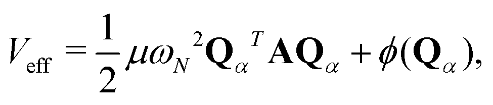
 being a harmonic chain frequency and A being a matrix whose the elements are described as Aij = 2δij − δi,j+1 − δi,j−1 with the cycle boundary conditions 0 → N and N + 1 → 1. The first term of the right-hand side of eqn (2) represents the harmonic interaction between the adjacent beads. The second term is the bead-averaged physical potential


 were transformed to (Qα,
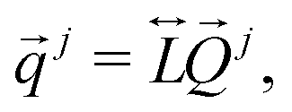
 is the 3n × 3n unitary matrix used to obtain the vibrational frequency diagonal matrix, Ω, diag(Ω) = (ω12, ⋯,ωα+62, ⋯,ω3n2). The Cartesian coordinates
  and their velocities for j-th bead can eventually be obtained by
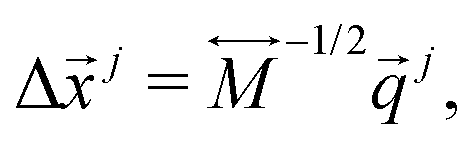
 being the 3n-dimensional Cartesian coordinate vector at the stationary point where is the TS in this study.
  is the diagonal matrix whose elements ml correspond to the atomic mass for the l-th Cartesian coordinate. Note that the centroid of beads is written by


 . The internal energy 〈Uc〉 therefore becomes


 of populating the state nvib with energy
  can be represented as