Improved modeling of anharmonicity for furan microsolvation†
Wassja A.
Kopp
 *,
Matthias L.
Mödden
*,
Narasimhan
Viswanathan
,
Gabriel
Rath
* and
Kai
Leonhard
*,
Matthias L.
Mödden
*,
Narasimhan
Viswanathan
,
Gabriel
Rath
* and
Kai
Leonhard

Institute of Technical Thermodynamics, RWTH Aachen University, 52062 Aachen, Germany. E-mail: kai.leonhard@ltt.rwth-aachen.de; Fax: +49 (0)241 80 92255; Tel: +49 (0)241 80 98174
First published on 30th March 2023
Abstract
Computational benchmark data for complexes requires accurate models of anharmonic torsional motion. State-of-the-art hindered rotor treatments come with a number of difficulties, regarding discontinuities from badly converged points or coupling, oscillations, or the consideration and correction of stationary points. Their manual handling introduces a level of arbitrariness not suitable for benchmark procedures. This study presents the TAMkinTools extension for improved modeling of one-dimensional hindered rotation which enables a more standardized workflow. We choose the structures from the Goebench challenge as test case, which comprises OH- and π-bonded complexes of methanol and furan, 2-methylfuran, and 2,5-dimethylfuran. Ahlrichs and Dunning basis sets of various sizes and their extrapolations show large differences in efficiency and accuracy for coupled-cluster energies of stationary points of these complexes. The probability density analysis of TAMkinTools provides zero-point energies for all conformations even within the same rotor profile. Zero-point energies show a large effect on the conformational order, especially for the methanol–furan complex with energy differences far below 1 kJ mol−1.
1 Introduction
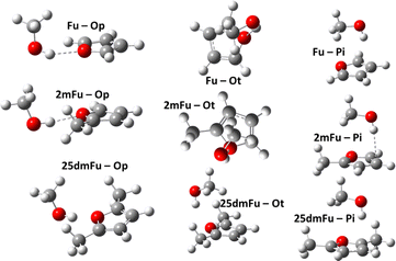
Theoretical modeling has become a crucial part of how new processes and compounds are developed today.1–3 Running model simulations for systems of interest can be orders of magnitude cheaper and faster than equipping laboratories to run real tests, so they serve a vital pre-screening role in technological discovery.4–6 Chemical modeling may contain numerous methods and models, depending on the involved molecules, temperatures, states of matter, and available human and computational resources. Developing new models or choosing an appropriate model often requires high-accuracy reference data in order to measure and compare model uncertainties. In turn, generating such high-accuracy reference data can itself be a major challenge, especially where real-world measurements are prohibitively expensive or unfeasible. This is one impetus behind so-called “benchmark challenges”, where a series of chemical modeling workflows are performed blindly on some specific systems for which high-accuracy experimental data is (made) available.7–11 These data are compared with the computational results and showcases how well each workflow is expected to perform for further, unknown, systems. An interesting target for benchmarking are the subtle energy differences appearing in intermolecular interactions with microsolvation. Such subtle energy differences show up e.g. in microsolvation of ions12 like Li+ with water,13 water–ammonia mixtures,14 methanol,15,16 and noble gases.17–19 Poblotzki et al.20 point out the particular relevance of furan derivate microsolvation in alcohols due to the interesting interplay of polar and non-polar docking sites. Dimers of furan derivates and alcohols or water have been investigated in a number of studies as pointed out by Gottschalk et al.,10 preferring OH-bonding with smaller, more polar partners,21–23 and π-bonding with larger alcohols,20,24,25 or being equally stable for both bonding patterns.26 These systems were used in the Goebench challenge9,10 to compare 12 different modeling workflows, looking at how well each could model the microsolvation of furan and furan-derivatives with methanol, cf.Fig. 1. This helps to determine which less-expensive model chemistries are still sufficient for producing accurate microsolvated geometries, vibrational frequencies, and especially (zero-point corrected) energies.When it comes to high-accuracy modeling of thermochemical data, including zero-point energies, one of the primary sources of uncertainties can be the treatment of contributions from the motions of nuclei. While uncertainties from electronic contributions can nowadays be rather easily reduced27–29 below 1 kJ mol−1, those arising from deficiencies in the commonly-used RRHO model for nuclear motions can be far greater, even when a highly-accurate electronic model is used.30–33 This was seen in the Goebench challenge9,10 as well, with the magnitude of the anharmonic corrections of the three tested workflows that used them regularly being near to or overshooting the ca. 1 kJ mol−1 uncertainty in CC-based electronic energies.
Nuclear motion can contribute differently to uncertainties in modeling workflows, but this paper focuses on one type of motion that is very common for systems larger than about five atoms: hindered rotation. This type of motion occurs as the concerted rotation of a set of atoms within a larger chemical system, usually either along σ bonds within a species. It plays an especially large role for the mutual rotation of two weakly bounded species within a transition state or a complex. RRHO's shortcomings in modeling these behaviors have been known for many decades,34–36 and these types of motions are usually responsible for many of the “low-frequencies” in RRHO calculations that are known to lead to gross uncertainties in partition functions and thus also errors in all thermochemical data.37 One very promising model that can handle these hindered rotations is the N × 1DHR model,31,38 which treats a species' various possible rotations as a combination of uncoupled 1DHR. In its implementation in the TAMkin python library,39 each of these rotors is obtained through Fourier curve fitting to a relaxed PES scan performed over the respective torsional coordinate. This software and the underlying N × 1DHR model has demonstrated good performance for a range of thermochemical28,40–42 and kinetic43,44 applications. However, several shortcomings prevent N × 1DHR approaches as implemented in TAMkin from being used more generally for generating reference data. For one, it is generally known that overfitting may occur in producing the potential energy curve, and the threshold in the number of Fourier functions past which overfitting can occur has to be determined on a case-by-case basis. This introduces some arbitrariness and handicaps application in benchmarking where it is crucial to maintain the same level of quality across different systems. Another issue is with dealing with discontinuities. These arise from cases where the relaxed scans used to construct the 1DHR move at some point along another dimension due to coupling introducing a sudden change in energy, and maybe upon further rotation even do not move out of these coupled region(s).28,43 Normally, these are dealt with by ignoring the data points through which a discontinuity manifests, but their manual determination and removal is error-prone and adds to the level of arbitrariness. A final drawback is the implicit lumping of all conformations linked by a scan into a single rotor. This prohibits to study the subtle energy differences of such conformations using N × 1DHR e.g. within a benchmark study.
For this study, we present our extension to the TAMkin library, TAMkinTools. It aims to address the above-mentioned limitations of TAMkin's implementation of the N × 1DHR model that have hampered its application to reference data suitable for benchmarking. The code contains an improved Fourier curve fitting procedure that eliminates the danger of overfitting from using too many functions. TAMkinTools also provides better support for dealing with discontinuities and (re)weighting data points in a more easily reproducible way. Furthermore, it adds support for performing Fourier curve fitting to data points taken at multiple fidelities, allowing to, e.g., introduce CC-level accuracy for all minima but still use faster model chemistries like DFT for modeling all other parts of configuration space. We then describe one possible, completely reproducible workflow enabled by these improvements within TAMkinTools. Finally, we apply this workflow to the original systems of interest in the Goebench challenge, i.e. that of dimers of methanol and furan, 2-methylfuran, and 2,5-dimethylfuran, cf.Fig. 1, and show how it can produce high-accuracy data without any need for case-by-case manipulations as long as the workflow is planned appropriately.
2. Theory
2.1 Thermochemistry from one-dimensional hindered rotor treatments
Chemical models contain reaction rate and equilibrium constants, which are related to (reactant, barrier, and product) free energy differences. The free energy A can be computed from the partition function Q according to A = −RT![[thin space (1/6-em)]](https://www.rsc.org/images/entities/i_char_2009.gif) ln(Q). Accurate computation of thermochemistry therefore requires accurate partition functions. For an ideal gas, within the standard Born–Oppenheimer and the RRHO approximations, the partition function factorizes into contributions from electronic energies, translation, rotation, and vibrational modes. Each of these contributions involves either a classical treatment, if applicable, or solving a reduced-dimensional SE, often analytically. To describe torsional motion, a HO model is usually inferior to an 1DHR approach. The 1DHR SE requires an accurate potential energy curve and the reduced moment of inertia and can then be solved numerically. While the reduced moment of inertia is usually statically determined from the optimized geometry at the global minimum, the potential energy along the torsional degree of freedom is recomputed at each of nscan dihedral angle values, often within constrained geometry optimizations.
ln(Q). Accurate computation of thermochemistry therefore requires accurate partition functions. For an ideal gas, within the standard Born–Oppenheimer and the RRHO approximations, the partition function factorizes into contributions from electronic energies, translation, rotation, and vibrational modes. Each of these contributions involves either a classical treatment, if applicable, or solving a reduced-dimensional SE, often analytically. To describe torsional motion, a HO model is usually inferior to an 1DHR approach. The 1DHR SE requires an accurate potential energy curve and the reduced moment of inertia and can then be solved numerically. While the reduced moment of inertia is usually statically determined from the optimized geometry at the global minimum, the potential energy along the torsional degree of freedom is recomputed at each of nscan dihedral angle values, often within constrained geometry optimizations.
Both the potential energy curve V and the basis functions for the 1DHR SE solutions ψ can be expressed as Fourier series of order N in rotation angle θ.
 | (1) |
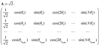 | (2) |
To add higher-fidelity points, e.g. from CC calculations performed at stationary points, we introduce an array of weighting factors. These weights can be increased for higher-fidelity points. Stationary point optimizations provide additional information beyond SPE, i.e. the gradient being zero. Inclusion of derivatives (as the gradient) of Fourier series into the fit is possible by extending the matrix A (eqn (2)) by rows containing the respective derivatives and extending the potential energy vector v by the respective value of the derivative, e.g. by zero. We also found that minimizing the second derivatives (curvature) along a grid of points avoids oscillations even when using a high number of Fourier functions. A fit according to all these different targets will of course result in a compromise, i.e. neither exactly reproduce all points nor restricting all gradients to exactly zero. Altogether, this leads to the optimized fitting prescription:
 | (3) |
As a by-product, because of the additional conditions, this allows for a higher number of Fourier basis functions, even higher than the number of computed points nscan. The lowest part of A and v, which corresponds to the second derivatives, can be evaluated for an arbitrary number of points so that the minimization problem can be solved for an arbitrary number of Fourier series elements.
TAMkinTools provides a means to analyze minima within the same potential energy curve by analysis of wavefunctions. In order to obtain populations (and from them further thermochemical data) of multiple minima, we divide a scan into ranges θi. Suitable limits for these ranges can be the dihedral angle values from transition state optimizations between the minima of interest. Then, we compute probabilities, i.e. populations, for all ranges for a given energy level E from the corresponding wavefunction:
 | (4) |
![[thin space (1/6-em)]](https://www.rsc.org/images/entities/char_2009.gif) θ + i
θ + i![[thin space (1/6-em)]](https://www.rsc.org/images/entities/i_char_2009.gif) sin
sin![[thin space (1/6-em)]](https://www.rsc.org/images/entities/char_2009.gif) θ. This allows to cast Fourier series elements of order n into complex exponentials according to:
θ. This allows to cast Fourier series elements of order n into complex exponentials according to:We call the resulting function type GFF and it represents a commutative ring.46 It can be converted back to a Fourier series:
c![[thin space (1/6-em)]](https://www.rsc.org/images/entities/i_char_2009.gif) exp(inθ) + d exp(inθ) + d![[thin space (1/6-em)]](https://www.rsc.org/images/entities/i_char_2009.gif) exp(−inθ) = (c + d)cos exp(−inθ) = (c + d)cos![[thin space (1/6-em)]](https://www.rsc.org/images/entities/char_2009.gif) nθ + (c − d) sin nθ + (c − d) sin![[thin space (1/6-em)]](https://www.rsc.org/images/entities/char_2009.gif) nθ nθ |
 | (5) |
This data allows to compute further thermochemical data or to weight other quantities of interest to benchmarking as spectroscopic features (e.g. frequency shifts), dipole moments, or rotational constants10 for each conformer on the 1DHR potential energy curve.
3. Methods
Geometries, 1D-scans and frequencies were obtained at B2PLYP-D3/6-311++g(d,p) level throughout. Stationary points, i.e. minima and TS, were optimized with the standard schemes but very tight convergence within the Gaussian09.d01 software.47 CCSD(T) SPE were calculated using ORCA 4.0.148 using the DLPNO approximation. We employed two different families of basis sets: Ahlrichs basis sets def2-TZVPP and def2-QZVPP and from that a def2-(T,Q)ZVPP extrapolation, and augmented Dunning basis sets aug-cc-pvdz, -pvtz, and pvqz, with extrapolations aug-cc-pv(d,t)z, and -pv(t,q)z.49,50 Detailed software settings and extrapolation formula are given in the ESI.†N × 1DHR motion is treated in this study using the TAMkin Python library version 1.2.639 and the TAMkinTools code developed in this study.The standard application procedure using TAMkinTools is as follows: the first step in our investigations is always the optimization of a molecular complex. Intermolecular interactions, e.g. leading to formation of dimers, usually provide six degrees of freedom (transitional modes) especially prone to anharmonicity.51 Within this study, we pick the hindered rotation of the two partners against each other, defined by a dihedral angle involving two adjacent atoms of each partner. Along this angle, a relaxed potential energy scan is performed. If a lower-energy minimum shows up during the scan, the procedure is repeated with its first step. For all minima in the scan, full optimizations, frequency and high-fidelity SPE calculations are performed. The energies of the stationary points are added with a weight of 100.0 while the standard weight is chosen to be 0.02 or 0.1 (discussed in Results section). At all stationary points the first derivatives in eqn (3) are required to be zero. For an evenly spaced grid of 1000 points, second derivatives are added in eqn (3) with target values of zero and a standard weight of 0.001. Then, the optimized rotor is set up with in this study always 14 Fourier functions; rotational symmetries are entered by the user. Finally, the SE is solved for a set of trial Fourier-type functions of sufficient size, from 100 to some thousand if one needs converged partition functions at high temperatures (in this study always 200). This also yields ZPE and all wavefunctions.
4. Results and discussion
4.1 Electronic energies
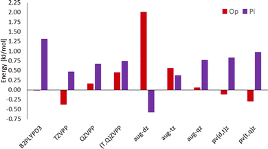
Hydrogen-bonded (OH) complexes (Ot and Op in Fig. 1) are energetically preferred over π-bonded complexes (PI in Fig. 1) for all structures in this study (this also holds for structures involving larger furan derivates which can be found in the ESI†). Fig. 2 shows that this holds for all methods compared in this study except for CC with aug-cc-pvdz basis set. That method also yields the largest deviations (1 kJ mol−1 to 3 kJ mol−1) from results with larger basis sets compared to all other methods in this study. On the other hand, extrapolation with aug-cc-pv(d,t)z bases is in most cases closer to the aug-cc-pv(t,q)z extrapolation than the aug-cc-pvqz energy itself. We choose the aug-(t,q)z extrapolation as a reference since it combines the largest basis sets used throughout this study.Different conformations of the OH-bonded complexes for larger furane derivates always energetically prefer the OH-bonded top configuration over the OH-bonded planar one. Only for the methanol–furane complex both hydrogen-bonded conformations are of comparable energy (cf.Fig. 2). The aug-cc-pv(t,q)z extrapolation even predicts the planar conformation to be favored. To clarify this, we performed additional CC calculations with an aug-cc-pv5z basis set which still predict the top configuration to be preferred by 0.01 kJ mol−1. Of course, a reliable calculation of such tiny energy differences must consider effects beyond a standard CCSD(T) treatment, e.g. core correlation and quadruple excitations27 which is beyond the scope of this study.
Energy differences obtained from the double-hybrid DFT functional B2PLYP and Grimmes D3BJ correction perform comparably well and deviate less than 1 kJ mol−1 from quadruple-ζ CC energies, except for some TS (all TS information is given in the ESI† since kinetics is beyond the scope of this study).
CC energies from Ahlrichs triple- and quadruple-ζ basis sets and their extrapolation is, while enabling relatively fast calculations, usually further from the aug-cc-pv(t,q)z extrapolation than the aug-cc-pv(d,t)z extrapolation. Although schemes for CC energy extrapolation using Ahlrichs basis sets have been proposed in the literature,49,50 correlation-consistent basis sets as Dunning's have been designed for extrapolation and consistently converge to results for even larger bases throughout this study.
4.2 Nuclear motion
Comparison of computed to experimental data even at 0 K must include nuclear (zero-point) motion models. While many modes of motion may be described sufficiently accurate by the RRHO model, this is usually not the case for torsion within the complex. HR modeling of this torsion can be improved and standardized using our TAMkinTools development.One frequent issue with modeling torsional motion comes from the afore-mentioned inconsistencies or jumps arising from coupling to other modes so that torsional scans may even not be periodic anymore. Furthermore, the scan or optimization of points therein may abort for various reasons. Such points appear for instance in the torsion of the OH-bonded methanol–furan complex, cf.Fig. 3.
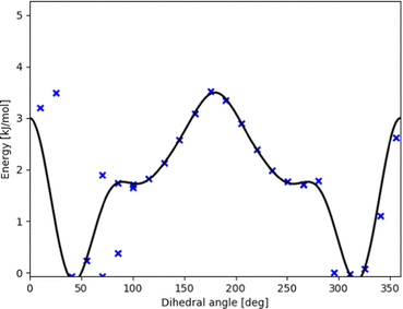 | ||
| Fig. 3 Potential energy curve (black line) fitted to represent DFT scan points (blue xs) along the intermolecular torsional angle in OH-bonded methanol–2,5-dimethylfuran. This profile was used in our contribution to the Goebench challenge.9,10 | ||
To remedy such inconsistencies, we removed points that do not match the symmetry of the profile or stem from coupling to other modes. Within our Goebench submission, we removed such points manually,9,10 while in this study we used the manipulation methods provided by TAMkinTools.
Further shortcomings of the standard HR treatment can be seen from Fig. 3: the minimum (near 310°) is shifted to the right and underpredicted. This has direct effect on energies, and in addition severely effects HR corrections because the curvature at the minimum is used to correct the HO part.
Fig. 4 contains scan points for the similar system of OH-bonded methanol–2-methylfurane. Here, we demonstrate the standardized workflow using eqn (3) within TAMkinTools, which yields an improved torsional profile: the fit represents all minima and stationary points at their optimized positions, yields a closed profile without oscillations, and includes high-fidelity points from CC (t,q)-ζ extrapolations. Of course, the scheme compromises between the conditions entering eqn (3), i.e. weighted scan points, stationary points and to-be-minimized curvature, so no single condition can be fulfilled to 100%.
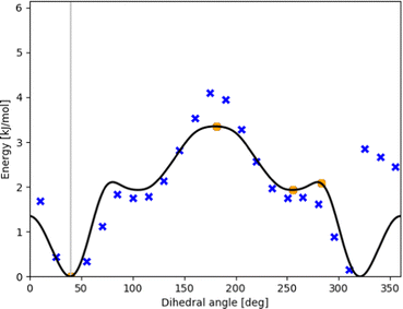 | ||
| Fig. 4 Potential energy curve (black line) fitted to represent DFT scan points (blue xs) as well as stationary points from CC calculations (orange circles) along the intermolecular torsional angle in OH-bonded methanol–2-methylfuran. This profile results from the fitting prescription in eqn (3). | ||
Fig. 5 shows further how the fit meets stationary points from a high-fidelity method while still maintaining the general shape of the potential energy curve even when a large number of low-fidelity points is used. The curve monotonously in- or decreases between maxima and minima (as it should when all stationary points are known). This is not yet forced explicitly by the optimized fit, so in principle beyond the vicinity of a stationary point the curve could be attracted by low-fidelity points and e.g. go further up from a maximum. Nevertheless, we had to adjust the standard point weight to be 0.02 or 0.1 in order to prevent this. Future development should include a corresponding restriction, together with optimized machine-learning multi-fidelity modeling.
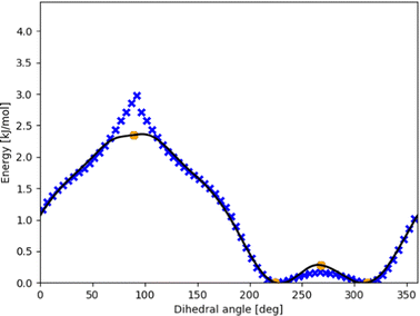 | ||
| Fig. 5 Dense DFT scan (blue xs) for the intermolecular torsion within the π-bonded methanol–furan complex with CC energies for the optimized stationary points (orange circles). The optimized fit (black line) using eqn (3) maintains the shape from the DFT points while monotonously and differentiably touching the stationary points. | ||
Because this study focuses on energies of minima and ZPE, the effect of including high-fidelity energies is not pronounced. We expect higher influence for results at finite temperature for thermochemistry and kinetics.
ZPE and finite-temperature thermochemistry and kinetics follow from the allowed energy levels of nuclear motion. For HR, these energy levels and the corresponding wavefunctions (in terms of Fourier series) result from solutions of torsional SE with TAMkin,39 requiring the potential energy curves discussed before and fixed moments of inertia derived from the reference geometry. These energy levels are properties of the whole rotor, comprising all conformations that appear in the scan. Probability density functions  reveal the fraction of systems hovering around a given dihedral angle θ for energy level E. TAMkinTools can plot these probability density functions for selected energy levels as depicted in Fig. 6. This allows to determine conformer-resolved quantities, including ZPE.
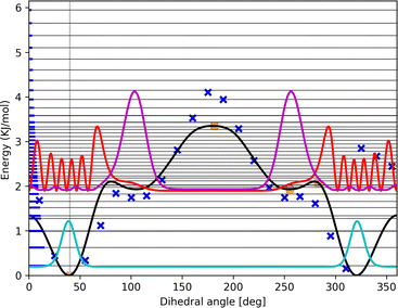 | ||
| Fig. 6 Three probability density functions shifted to their corresponding energy level for energy levels 0 (cyan line), 11 (red line), and 12 (magenta line) of the OH-bonded methanol–2-methylfuran torsion from Fig. 4. The horizontal thin black lines depict the energy levels while the bold blue parts on the left represent the population of the respective energy level according to the Boltzmann distribution at 298.15 K. The wells from −77.2° to 0° and from 0° to 77.2° correspond to the top Ot conformation at ±40° while the wells from 77.2° to 180° and from 180° to −77.2° correspond to the planar Op conformation at ±104.9°. | ||
ZPE and potential energies determine preferred structures at 0 K. All ZPE and selected population density profiles are given in the ESI.† For all complexes in this study, OH-bonded conformations are preferred over π-bonded conformations, both regarding potential energies and ZPE, cf.Table 1. ZPE at RRHO level also resolve the two different OH-bonded conformations. While for larger furans the Ot structure is preferred, for methanol–furan the Op structure shows lowest energy at 0 K, in contradiction to experimental findings. The experimental rotational spectroscopy results discussed by Gottschalk et al.10 clearly point to preference of the top Ot conformation. The two OH-bonded conformations (top and planar) may be compared within the HR model using the first energy level for which a significant population peak is visible within the respective well (for methanol–2-methylfuran for example, this would be level 12, not 11, cf.Fig. 6). Here, using the HR model, only inclusion of wave function analysis can tell which lowest energy level is populated by which conformer. Also these conformer-resolved ZPE always favor the top structure Ot (as do the high-fidelity potential energies) except for the methanol–furan case. The two OH-bonded methanol-furane conformations have almost identical potential energies, and inclusion of ZPE even points in favor of the planar Op conformation. The energy at 0 K is computed to be lower by 0.5 kJ mol−1 for aug-cc-pv(t,q)z extrapolation and by 0.24 kJ mol−1 for the aug-cc-pv5z potential energy surface. The dominating contribution to this energy difference, about 0.2 kJ mol−1, though comes from the vibrational ZPE for the remaining modes from the RRHO model. Anharmonicity from HR model already slightly changes the energy at 0 K in the correct direction.
| Structure | RRHO | Direct fit | Opt. fit | Exp.10 |
|---|---|---|---|---|
| Me–Fu Ot | 0.55 | 0 | 0.49 | 0 |
| Me–Fu Op | 0 | — | 0 | Unpref. |
| Me–Fu PI | 0.69 | 0.19 | 0.44 | 0.42 ± 0.58 |
| Me-2mFu Ot | 0 | 0 | 0 | n.a. |
| Me-2mFu Op | 1.56 | — | 1.52 | n.a. |
| Me-2mFu PIa | 0.98 | 0.78 | 0.99 | n.a. |
| Me-2mFu PIb | 1.28 | — | 1.29 | n.a. |
| Me-25dmFu Ot | 0 | 0 | 0 | 0 |
| Me-25dmFu Op | 2.07 | — | 1.92 | Unpref. |
| Me-25dmFu PI | 0.91 | 0.92 | 0.86 | 0.34 ± 0.50 |
The experimentally favored Ot configuration shows a wider, more unsymmetric well in the HR scans and an anharmonicity treatment that includes further vibrational modes could affect the lion's share of ZPE contribution, i.e. the RRHO part, in favor of the experimentally correct Ot conformation.
A population analysis according to eqn (4) on the aug-cc-pv(t,q)z PES shows that also at finite temperature the planar Op conformation is preferred, at 10 K by 95.6% and at 298.15 K by 67%. The present analysis of eqn (4) only refers to the 1DHR profile and does not account for coupling and frequency changes of the other modes. In the 1DHR profile, the planar Op conformation occupies a broader well which explains its preference also at finite temperature. Within a more-dimensional picture that would include the top vs. planar interconversion in addition to the mutual rotation and changes in vibrational frequencies, the accessible configuration space volume of each conformation may again be different.
Shallow energy differences as between the two OH-bonded conformations in methanol–furan below 0.5 kJ mol−1 provide a particularly interesting target for even higher-level benchmark tests far below an uncertainty of 1 kJ mol−1. On the computational side, this would require both highly accurate electronic energies including core correlation and higher excitations as well as more sophisticated anharmonicity treatments that include (coupling to) further vibrational modes. A collection of similarly narrow-spaced conformers or isomers as next-generation benchmark set could foster the development of computational chemistry methods beyond what is currently termed chemical accuracy.
5. Conclusions
Nuclear motion models, especially for intermolecular torsions, are crucial for benchmark calculations. One-dimensional hindered rotor treatments often require manual intervention and suffer from numerical fitting problems, convergence problems in scans, and analysis limitations for results of multiple fidelities and multiple conformations. The TAMkinTools extension presented in this study remedies these drawbacks and enables a standardized workflow to be used for benchmark calculations. The workflow is applied to the methanol–furan derivate complexes known from the Goebench study.9,10 Coupled-cluster energies with the DLPNO approximation provide accurate energy corrections when used with Dunning basis sets; the augmented double- and triple-ζ basis set extrapolation proves to be particularly efficient. TAMkinTools provides smooth potential energy curves that can account for coupled-cluster correction data and provides a wavefunction analysis which can be used to attribute ZPE to individual conformations within the same rotor. For OH-bonded methanol–furan, the energy difference at 0 K between conformations is far below 1 kJ mol−1 even at the highest levels of theory and makes the correct reproduction of experimental orders (top lower than planar) challenging. Such conformations may be subject to next-level benchmarks for energy differences below 1 kJ mol−1, where computational chemistry methods require coupled anharmonic treatments of further librational modes.Author contributions
Wassja A. Kopp: methodology, software, validation, formal analysis, investigation, writing – original draft, Matthias L. Mödden: software, validation, investigation, Narasimhan Viswanathan: software, visualization, data curation, Gabriel Rath: writing – review & editing, Kai Leonhard: resources, conceptualization, writing – original draft, supervision, project administration, funding acquisition.Conflicts of interest
There are no conflicts to declare.Acknowledgements
We gratefully acknowledge support by student coworkers Tim Pilz, Ekaterina Mazur, and Dmitrii Tolmachev. Simulations were performed with computing resources granted by RWTH Aachen University under project rwth0070. Wassja Kopp acknowledges funding by the Deutsche Forschungsgemeinschaft (DFG, German Research Foundation) under Germany's Excellence Strategy – Cluster of Excellence 2186 “The Fuel Science Center” – ID: 390919832. Narasimhan Viswanathan acknowledges funding by the German Research Foundation for the project “Ab initio Thermochemistry and Kinetics of Molecules with Coupled Large-Amplitude Motions” – ID: 403683184. Gabriel Rath acknowledges funding from the European Unions Horizon 2020 research and innovation programme under grant agreement “Automatic Generation of Chemical Models” no. 814143.Notes and references
- E. I. Izgorodina and M. L. Coote, Chem. Phys., 2006, 324, 96–110 CrossRef CAS.
- J. Zador, C. A. Taatjes and R. X. Fernandes, Prog. Energ. Combust., 2011, 37, 371–421 CrossRef CAS.
- M. Stamatakis, J. Phys.-condens. Mat., 2015, 27, 1–28 Search PubMed.
- J. A. H. Schwöbel, M. Preißinger, D. Brüggemann and A. Klamt, Ind. Eng. Chem. Res., 2017, 56, 788–798 CrossRef.
- J. Schilling, D. Tillmanns, M. Lampe, M. Hopp, J. Gross and A. Bardow, Mol. Syst. Des. Eng., 2017, 2, 301–320 RSC.
- C. Gertig, E. Erdkamp, A. Ernst, C. Hemprich, L. Kroger, J. Langanke, A. Bardow and K. Leonhard, ChemistryOpen, 2021, 10, 534–544 CrossRef CAS PubMed.
- R. A. Mata and M. A. Suhm, Angew. Chem., Int. Ed., 2017, 56, 11011–11018 CrossRef CAS PubMed.
- M. Schappals, A. Mecklenfeld, L. Kröger, V. Botan, A. Koester, S. Stephan, E. J. Garcia, G. Rutkai, G. Raabe, P. Klein, K. Leonhard, C. W. Glass, J. Lenhard, J. Vrabec and H. Hasse, J. Chem. Theor. Comput., 2017, 13, 4270–4280 CrossRef CAS PubMed.
- H. C. Gottschalk, A. Poblotzki, M. A. Suhm, M. M. Al-Mogren, J. Antony, A. A. Auer, L. Baptista, D. M. Benoit, G. Bistoni, F. Bohle, R. Dahmani, D. Firaha, S. Grimme, A. Hansen, M. E. Harding, M. Hochlaf, C. Holzer, G. Jansen, W. Klopper, W. A. Kopp, L. C. Kröger, K. Leonhard, H. Mouhib, F. Neese, M. N. Pereira, I. S. Ulusoy, A. Wuttke and R. A. Mata, J. Chem. Phys., 2018, 148, 014301 CrossRef PubMed.
- H. C. Gottschalk, A. Poblotzki, M. Fatima, D. A. Obenchain, C. Pérez, J. Antony, A. A. Auer, L. Baptista, D. M. Benoit, G. Bistoni, F. Bohle, R. Dahmani, D. Firaha, S. Grimme, A. Hansen, M. E. Harding, M. Hochlaf, C. Holzer, G. Jansen, W. Klopper, W. A. Kopp, M. Krasowska, L. C. Kröger, K. Leonhard, M. Mogren Al-Mogren, H. Mouhib, F. Neese, M. N. Pereira, M. Prakash, I. S. Ulusoy, R. A. Mata, M. A. Suhm and M. Schnell, J. Chem. Phys., 2020, 152, 164303 CrossRef CAS PubMed.
- T. L. Fischer, M. Bödecker, A. Zehnacker-Rentien, R. A. Mata and M. A. Suhm, Phys. Chem. Chem. Phys., 2022, 24, 11442–11454 RSC.
- C. Hadad, E. Florez, N. Acelas, G. Merino and A. Restrepo, Int. J. Quantum Chem., 2019, 119, e25766 CrossRef.
- J. Romero, A. Reyes, J. David and A. Restrepo, Phys. Chem. Chem. Phys., 2011, 13, 15264–15271 RSC.
- S. Pratihar and A. Chandra, J. Chem. Phys., 2008, 129, 024511 CrossRef PubMed.
- C.-C. Wu, Y.-S. Wang, C. Chaudhuri, J. Jiang and H.-C. Chang, Chem. Phys. Lett., 2004, 388, 457–462 CrossRef CAS.
- J. Llanio-Trujillo, J. Marques and F. Pereira, Comput. Theor. Chem., 2013, 1021, 124–134 CrossRef CAS.
- M. Rastogi, C. Leidlmair, L. An der Lan, J. Ortiz de Zárate, R. Pérez de Tudela, M. Bartolomei, M. I. Hernández, J. Campos-Martínez, T. González-Lezana, J. Hernández-Rojas, J. Bretón, P. Scheier and M. Gatchell, Phys. Chem. Chem. Phys., 2018, 20, 25569–25576 RSC.
- W. S. Jesus, F. V. Prudente and J. M. C. Marques, J. Phys. Chem. A, 2019, 123, 2867–2873 CrossRef CAS PubMed.
- M. Slama, H. Habli, M. Laajimi, H. Ghalla and M. Ben El Hadj Rhouma, J. Mol. Graphics Modell., 2022, 116, 108229 CrossRef CAS PubMed.
- A. Poblotzki, J. Altnoder and M. A. Suhm, Phys. Chem. Chem. Phys., 2016, 18, 27265–27271 RSC.
- E. Sánchez-García, A. Mardyukov, M. Studentkowski, L. A. Montero and W. Sander, J. Phys. Chem. A, 2006, 110, 13775–13785 CrossRef PubMed.
- S. P. Lockwood, T. G. Fuller and J. J. Newby, J. Phys. Chem. A, 2018, 122, 7160–7170 CrossRef CAS PubMed.
- X. Jiang, N. T. Tsona, S. Tang and L. Du, Spectrochim. Acta, Part A, 2018, 191, 155–164 CrossRef CAS PubMed.
- A. Poblotzki, H. C. Gottschalk and M. A. Suhm, J. Phys. Chem. Lett., 2017, 8, 5656–5665 CrossRef CAS PubMed.
- D. Bernhard, M. Fatima, A. Poblotzki, A. L. Steber, C. Pérez, M. A. Suhm, M. Schnell and M. Gerhards, Phys. Chem. Chem. Phys., 2019, 21, 16032–16046 RSC.
- H. Sasaki, S. Daicho, Y. Yamada and Y. Nibu, J. Phys. Chem. A, 2013, 117, 3183–3189 CrossRef CAS PubMed.
- A. Tajti, P. G. Szalay, A. G. Császár, M. Kallay, J. Gauss, E. F. Valeev, B. A. Flowers, J. Vázquez and J. F. Stanton, J. Chem. Phys., 2004, 121, 11599–11613 CrossRef CAS PubMed.
- M. Umer and K. Leonhard, J. Phys. Chem. A, 2013, 117, 1569–1582 CrossRef CAS PubMed.
- N. Sylvetsky, K. A. Peterson, A. Karton and J. M. L. Martin, J. Chem. Phys., 2016, 144, 214101 CrossRef PubMed.
- A. L. L. East, B. J. Smith and L. Radom, J. Am. Chem. Soc., 1997, 119, 9014–9020 CrossRef CAS.
- V. Van Speybroeck, P. Vansteenkiste, D. Van Neck and M. Waroquier, Chem. Phys. Lett., 2005, 402, 479–484 CrossRef CAS.
- S. Sharma, S. Raman and W. H. Green, J. Phys. Chem. A, 2010, 114, 5689–5701 CrossRef CAS PubMed.
- A. Fernández-Ramos, J. Chem. Phys., 2013, 138, 134112 CrossRef PubMed.
- K. S. Pitzer, J. Chem. Phys., 1937, 5, 469–472 CrossRef CAS.
- K. S. Pitzer and W. D. Gwinn, J. Chem. Phys., 1942, 10, 428–440 CrossRef CAS.
- D. G. Truhlar, J. Comput. Chem., 1991, 12, 266–270 CrossRef CAS.
- E. Dzib and G. Merino, Wiley Interdiscip. Rev.: Comput. Mol. Sci., 2021, e1583 Search PubMed.
- P. Vansteenkiste, V. Van Speybroeck, G. B. Marin and M. Waroquier, J. Phys. Chem. A, 2003, 107, 3139–3145 CrossRef CAS.
- A. Ghysels, T. Verstraelen, K. Hemelsoet, M. Waroquier and V. van Speybroeck, J. Chem. Inf. Model., 2010, 50, 1736–1750 CrossRef CAS PubMed.
- M. Umer, W. A. Kopp and K. Leonhard, J. Chem. Phys., 2015, 143, 214306 CrossRef PubMed.
- L. C. Kröger, S. Müller, I. Smirnova and K. Leonhard, J. Phys. Chem. A, 2020, 124, 4171–4181 CrossRef PubMed.
- G. Rath, W. A. Kopp and K. Leonhard, J. Chem. Inf. Model., 2021, 61, 5853–5870 CrossRef CAS PubMed.
- W. A. Kopp, R. T. Langer, M. Döntgen and K. Leonhard, J. Phys. Chem. A, 2013, 117, 6757–6770 CrossRef CAS PubMed.
- L. C. Kröger, W. A. Kopp and K. Leonhard, J. Phys. Chem. B, 2017, 121, 2887–2895 CrossRef PubMed.
- W. A. Kopp and K. Leonhard, J. Chem. Phys., 2016, 145, 234102 CrossRef PubMed.
- W. A. Kopp, PhD thesis, RWTH Aachen University, Aachen, 2018.
- M. J. Frisch, G. W. Trucks, H. B. Schlegel, G. E. Scuseria, M. A. Robb, J. R. Cheeseman, G. Scalmani, V. Barone, B. Mennucci, G. A. Petersson, H. Nakatsuji, M. Caricato, X. Li, H. P. Hratchian, A. F. Izmaylov, J. Bloino, G. Zheng, J. L. Sonnenberg, M. Hada, M. Ehara, K. Toyota, R. Fukuda, J. Hasegawa, M. Ishida, T. Nakajima, Y. Honda, O. Kitao, H. Nakai, T. Vreven, J. A. Montgomery, Jr., J. E. Peralta, F. Ogliaro, M. Bearpark, J. J. Heyd, E. Brothers, K. N. Kudin, V. N. Staroverov, R. Kobayashi, J. Normand, K. Raghavachari, A. Rendell, J. C. Burant, S. S. Iyengar, J. Tomasi, M. Cossi, N. Rega, J. M. Millam, M. Klene, J. E. Knox, J. B. Cross, V. Bakken, C. Adamo, J. Jaramillo, R. Gomperts, R. E. Stratmann, O. Yazyev, A. J. Austin, R. Cammi, C. Pomelli, J. W. Ochterski, R. L. Martin, K. Morokuma, V. G. Zakrzewski, G. A. Voth, P. Salvador, J. J. Dannenberg, S. Dapprich, A. D. Daniels, O. Farkas, J. B. Foresman, J. V. Ortiz, J. Cioslowski and D. J. Fox, Gaussian 09 Revision D.01, 2009, Gaussian Inc., Wallingford CT, 2009 Search PubMed.
- F. Neese, Wiley Interdiscip. Rev.: Comput. Mol. Sci., 2012, 2, 73–78 CAS.
- F. Neese and E. F. Valeev, J. Chem. Theory Comput., 2011, 7, 33–43 CrossRef CAS PubMed.
- D. G. Liakos, M. Sparta, M. K. Kesharwani, J. M. L. Martin and F. Neese, J. Chem. Theory Comput., 2015, 11, 1525–1539 CrossRef CAS PubMed.
- D. M. Wardlaw and R. A. Marcus, Chem. Phys. Lett., 1984, 110, 230–234 CrossRef CAS.
Footnote |
| † Electronic supplementary information (ESI) available: SITT.pdf lists all structures, energies, and hindered rotor results from this work, TAMkinTools.zip contains the software python code (also available from https://git.rwth-aachen.de/Wassja.Kopp/tamkintools/-/releases/1_0PCCP, and SI.zip contains all hindered rotor sample calculations from this work. See DOI: https://doi.org/10.1039/d2cp03907a |
| This journal is © the Owner Societies 2023 |

