Molecular cluster analysis using local order parameters selected by machine learning
Received
11th August 2022
, Accepted 9th November 2022
First published on 9th December 2022
Abstract
Accurately extracting local molecular structures is essential for understanding the mechanisms of phase and structural transitions. A promising method to characterize the local molecular structure is defining the value of the local order parameter (LOP) for each particle. This work develops the Molecular Assembly structure Learning package for Identifying Order parameters (MALIO), a machine learning package that can propose an optimal (set of) LOP(s) quickly and automatically for a huge number of LOP species and various methods of selecting neighboring particles for the calculation. We applied this package to distinguish between the nematic and smectic phases of uniaxial liquid crystal molecules, and selected candidate LOPs that could be used to precisely observe the nematic–smectic phase transition. The LOP candidates were used to observe the nucleation and subsequent percolation transition, and the effect of the choice of LOP species and neighboring particles on the statistics of local molecular structures (clusters) was examined. The procedure revealed the time evolution of the number of clusters and the dependence of the percolation curve on the number of neighboring particles for each LOP species. The LOP species with the lowest dependence on the number of neighboring particles was the best-performing LOP species in the MALIO screening strategy. These results not only show that machine learning can powerfully screen a huge number of LOP species and suggest only a few promising candidates, but also indicate that MALIO can select the best LOP species.
1 Introduction
Phase transitions have been studied not only in condensed matter physics,1 but also in a wide range of fields including biology and engineering.2–6 In particular, controlling the rate at which the transition occurs has been a subject of interest for many years, not only because it directly affects the applicability of materials to devices in which the transition is an important part of the mechanism,7,8 but also because it affects the speed of material generation and processing for higher yields of desirable material structures and prevention of undesirable structuring.9–12 Regardless of whether the process is a first-order phase transition or phase separation, it is important to focus on local molecular structures to understand the transition phenomena. In phase transitions, the local structures occur in the bulk or at the interface before the transition, and often have post-transitional structural motifs.1,11,13–21 Attempts to understand transition kinetics from the time evolution of the size and shape statistics of local molecular structures (clusters) have been made for many years and yielded many valuable results.16,17,22–32 Such cluster analysis is supported by precisely extracting local molecular structures. For simple materials such as noble gases and metals, it is relatively easy to extract the local molecular structure by selecting local density differences.33,34 However, ordering of materials with high electrostatic and molecular shape anisotropy, such as water, silica, liquid crystals, and polymers, is much more complex, and it is difficult to characterize differences in various ordered structures in terms of local density differences. For such problems, global order parameters have been sometimes used to justify cluster analysis based on slight differences in local density, but the limitations of this strategy have already been reported.26,35 Recall that the global order parameter, by its definition, gives a simple value that indicates the degree of order in the entire molecular system, and thus the global order parameter alone cannot detect the local structure inside a molecular system. More recently, attempts have been made to define order parameter values for individual atoms and molecules (i.e., local order parameters (LOPs)) and to characterize local molecular structures in more detail. LOPs were first developed to distinguish basic crystal structures such as body-centered cubic, face-centered cubic, hexagonal close-packed, and glass,36–42 and is now a promising method to distinguish various molecular structures.26,30,32,35,39,43–48 The advantage of an LOP is that it is possible to quantitatively determine which structure a material belongs to for each of its constituents (such as atoms, molecules, and coarse-grained particles). This allows us to reveal local molecular structures and their distributions with very high resolution. In fact, several studies have already demonstrated that LOP can track self-organization dynamics during phase transitions.26,30,32,35,49 Furthermore, it has been reported that 3D molecular coordinate data can be obtained from experiments and LOP values can be calculated to analyze experimental results.50 However, information on neighboring particles is essential for calculating an LOP value. Therefore, the amount of information on neighboring particles affects the accuracy of the LOP value and thus the extraction of local molecular structures. As the number of neighboring particles increases, the LOP value may become more robust and the accuracy of structure determination may increase, while the resolution of local molecular structures may decrease. This trade-off between the number of neighboring particles and resolution has often been discussed in calculating LOP values,35,51 but a unified view has not yet been obtained. Another problem is that the effective LOP species for a particular substance or phase structure is not self-evident, so it is necessary to select the best one from a huge number of LOP candidates.32,42,45–48
This work develops the molecular assembly structure learning package for identifying order parameters (MALIO), a machine learning package that can quickly and automatically suggest the optimal LOPs and LOP combinations for various protocols for selecting neighboring particles. MALIO is based on the machine learning-aided local structure analyzer (ML-LSA),32,45 but attempts to speed up LOP calculations by completely re-coding in Cython52 and improving related libraries. To evaluate the performance of LOP selection by MALIO, we focus on the nematic–smectic transition of uniaxial liquid crystal molecules. The nematic–smectic transition is a first-order phase transition. It has long been known that nucleation occurs in the early stage of the first-order phase transition, regardless of the substance.1 Nucleation is a phenomenon in which the phase transition proceeds only when molecular clusters of a certain size are generated.1 Therefore, the existence of molecular clusters with short-range order (CCs: cybotactic clusters) in the early stages of the liquid crystal phase transition has long been proposed and has been measured using X-rays in uniaxial and bent-core liquid crystal systems.53,54 However, the shape and role of CCs during phase transitions have long remained unclear. Molecular cluster analysis applying LOP to trajectories of phase transition dynamics obtained from molecular dynamics simulations has revealed for the first time the shape and role of CCs during the phase transition.32 A similar analysis has also been attempted for the isotropic-nematic transition.55 MALIO is applied to distinguish between nematic and smectic phases of uniaxial liquid crystal molecules, and candidate LOPs are selected for each protocol for selecting neighboring particles. The selected LOP candidates are used to observe the nucleation and subsequent percolation transition, and the impact of both the LOP species and the protocols on cluster statistics are investigated. Note that although defect formation and destruction occur during the liquid crystal phase transition,56,57 it is difficult to observe defects on the scale of an optical microscope in molecular simulations. Especially in the case of the smectic phase, nothing can be said about layer defects unless it is possible to identify which molecular assemblies constitute a single smectic layer. Also, from a molecular point of view, the formation and destruction of defects is likely to be a phenomenon that occurs at least further after the percolation transition that occurs after nucleation. Therefore, it is outside the scope of this work.
2 Methodology
2.1 Molecular dynamics simulations
Molecular dynamics (MD) simulations of the liquid crystal phase transition were performed using the Soft-Core Gay-Berne (SCGB) model in the large-scale atomic/molecular massively parallel simulator (LAMMPS).58 The pairwise interaction potential of the SCGB model, USCGB, is expressed by the equations| | | USCGB = (1 − f)UGB + fUSC, | (1) |
| | | f = 1/{1 + exp[b(σa − r)]}, | (2) |
| |  | (3) |
where f is a sigmoidal logistic function, UGB is the pairwise interaction potential of the ellipsoidal GB particles, εa denotes the anisotropic energy of an ellipsoidal pair, r is the distance between the centers of mass of a pair of particles, σa is the anisotropic length of the ellipsoidal pair, σs is the length of the side-by-side configuration of the ellipsoids, USC is the soft-core potential energy, a is the potential slope of the soft repulsive energy barrier, and b is the steepness of the sigmoidal logistic seaming function. By introducing the parameter κ = σe/σs, in which σe denotes the length of the end-to-end configuration of the ellipsoids, we can write the anisotropic energy εa as| |  | (5) |
where ε denotes the characteristic well depth of the interaction potential,  and
and  denote the contributions corresponding to the well depth and configuration anisotropies, and μ and ν are multipliers for determining these two contributions to the pair potential. The factor
  is characterized by introducing a parameter
  , where
  and
and  denote energy contributions from the end-to-end and side-by-side ellipsoid configurations, respectively. The factor
  is characterized by κ. Therefore, the detailed shape of UGB is determined from the values of the four parameters κ, κ′, μ, and ν. We set κ = 3, κ′ = 5, μ = 1, and ν = 3. Note that the above parameter set has been traditionally used because the physical properties of nematic and smectic B liquid crystal phases are well displayed.59,60 For the characteristic length, energy, and mass of the SCGB systems, σ = σs, ε = kBT, and m are each set to 1; here, m is the mass of one SCGB particle. The terms a and b were set to −70εσ−1 and −100σ−1, respectively, on the basis of previous reports.60,61 Using the above parameter settings, the nematic–smectic transition is guaranteed to be observed for SCGB systems by quenching from temperature T = 2.4 to 1.8 at a density of 0.3σ−3.60 Therefore, an ensemble was used having a constant number of particles at a density of 0.3σ−3 contained within a cubic box of constant volume and temperature with full periodic boundary conditions imposed. The initial configurations for the nematic–smectic phase transition trajectory were prepared carefully by being cooled gradually from the isotropic phase at T = 6.0 to the nematic phase at T = 2.4. The configurations were then quenched to T = 1.8 below the nematic–smectic transition temperature TN–Sm = 2.25. To observe the fast nucleation during the weak first-order phase transition, a velocity Verlet integrator with a fine timestep of 2.0 × 10⁻⁵τ was used for SCGB, where τ = (mσ/ε)1/2 is a time unit. The temperature was controlled using a Nosé–Hoover chain thermostat.62 The SCGB potential was truncated at 8.0σ to precisely compute the intermolecular interactions during the phase transition.
2.2 Local order parameters
MALIO implements 17 typical definition functions of LOPs that have been developed individually and are introduced below. Note that most of the LOPs have internal parameters, and a huge number of LOPs can be considered by changing these parameters.
The neighborhood parameter A was developed by Honeycutt and Andersen63,64 and by Radhi and Behdinan41 to characterize the crystal structure of Lennard-Jones fluid based on the distance between the pair particles and its neighbor particles. A is expressed as
| |  | (6) |
| |  | (7) |
| |  | (8) |
where
Nb(
i) is an array that stores the identifiers of neighbor beads of bead
i in order of decreasing distance from bead
i,
Nb(
i,
j) is an array including the identifiers of mutually neighboring particles of particles
i and
j,
N and
M denote the numbers of elements in arrays
Nb(
i) and
Nb(
i,
j), and
rij is a vector from particle
j to particle
i. We consider
M = 1, 2, and 3. MALIO uses local averaging to improve the accuracy of molecular structure classification by LOPs. The “locally averaged” neighborhood parameter
Ā is defined as
| |  | (9) |
where the superscript “var” indicates the variation of
A from 1 to 3, and
Ñb(
i) is an array including the identifiers of neighboring particles and particle
i. The local averaging is based on
Ñb and does not lead to an increase in the effective number of neighboring particles. This process is the same as that used for spherical harmonic functions in the modified bond-orientational order parameters used by Lechner and Dellago,
39 described below. The neighbors of particle
i are not the same as those of particle
j. From this uniqueness of
Ñb, the LOP values for particles
i and
j are different regardless of the local averaging process. Importantly, differences in the LOP values determine the resolution at which we can distinguish local molecular structures. Thus, excessively repeating the averaging operation does cause any loss of local information by diminishing the differences.
The bond-angle order parameter B was used by Ackland and Jones38 to identify dislocation defects in colloidal suspensions based on the bond angle between the central particle and its neighbor particles. B is expressed as
| |  | (10) |
| | | f(θjik) = cosn1(n2θjik + ϕ), | (11) |
where
θjik is the angle between
rij and
rik,
n1 and
n2 are positive integers, and
ϕ is an offset angle. We consider
n1 = 1 and 2;
n2 = 1, 2, and 3; and
ϕ = 0, 2/3π, π/2, π/3, π/4, π/5, and π/6. The locally averaged neighborhood parameter
![[B with combining macron]](https://www.rsc.org/images/entities/i_char_0042_0304.gif)
is defined as
| |  | (12) |
The centrosymmetry parameter C was used by Kelchner and co-workers37 to analyze dislocations and defects on metal surfaces based on the distance between the central particle and its neighbor particles. C is expressed as
| |  | (13) |
where

is an array including the identifiers of neighbor beads of half of
Nb(
i) in order of nearest neighbor from particle
i,
N′ denotes the number of elements in array

and
k satisfies the relation
k =
j +
N −
N′. The locally averaged neighborhood parameter
![[C with combining macron]](https://www.rsc.org/images/entities/i_char_0043_0304.gif)
is defined as
| |  | (14) |
The neighbor distance parameter D was used by Stukowski40 to identify the crystal structure at grain boundaries by introducing a scale factor related to the distance of neighbor particles. D is expressed as
| |  | (15) |
where
r is the interparticle distance, and
fα,
fβ, and
fγ are the scale factor functions of
r. In MALIO,
fα,
fβ, and
fγ can be freely defined by users as scalar functions of
r.
Table 1 shows the functions represented by
fα,
fβ, and
fγ in this work. In the following sections, the specific form of
fα,
fβ, or
fγ corresponds to the function listed for each subscript of the parameters in
Table 1. Note that
α,
β, and
γ correspond to the subscript numbers of the function
f in
Table 1, respectively. The locally averaged neighborhood parameter
![[D with combining macron]](https://www.rsc.org/images/entities/i_char_0044_0304.gif)
is defined as
| |  | (16) |
Table 1 Functions represented by fα, fβ, and fγ
| Function |
Formula |
|
f
1
|
r
|
|
f
2
|
r
2
|
|
f
3
|

|
The angular Fourier series parameter F was developed by Bartok and co-workers43,44 to analyze potential energy surfaces in bulk crystals and silicon based on periodic properties of the structure. F is expressed as
| | 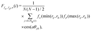 | (17) |
where
a is an angular factor. We consider
a = 1.0, 2.0, 3.0, 4.0, 6.0, 8.0, π/
ϕ0, 2π/
ϕ0, 3π/
ϕ0, 4π/
ϕ0, and 6π/
ϕ0, where
ϕ0 = 109.5π/180. The locally averaged neighborhood parameter
![[F with combining macron]](https://www.rsc.org/images/entities/i_char_0046_0304.gif)
is defined as
| |  | (18) |
The angle histogram parameter H developed in previous work45 is expressed as
| | | Hν(i) = FTampl.(h(θjik))δ(τ − ν), | (19) |
where
FTampl. is the amplitude function after a Fourier transform,
h is a function representing the histogram,
δ is the Dirac delta function, and
ν is the frequency of the Dirac delta function. We consider
ν = 1.0, 2.0, 3.0, 4.0, 5.0, 6.0, 7.0, 8.0, and 12.0. The locally averaged angle histogram parameter
![[H with combining macron]](https://www.rsc.org/images/entities/i_char_0048_0304.gif)
is defined as
| |  | (20) |
The tetrahedral order parameter I was developed by Chau and Hardwick65,66 to evaluate the tetrahedral configurations of molecules and was applied to water, methane and Lennard-Jones fluids. I is expressed as
| |  | (21) |
The locally averaged neighborhood parameter
Ī is defined as
| |  | (22) |
The bond-orientational order parameters QS and WS, based on spherical harmonic functions, were originally developed by Steinhardt and co-workers36 to quantitatively evaluate the orientational order of supercooled liquids and metallic glasses. QS and WS are expressed as
| |  | (23) |
| |  | (24) |
| |  | (25) |
where
l is an arbitrary positive integer denoting the degree of the harmonic function,
m is an integer that runs from −
l to +
l, and
Ylm is a spherical harmonic function. We consider
l = 2, 3, 4, 5, 6, 7, 8, 9, 10, 11, 12, 13, 14, 15, 16, 18, and 24. It is worth noting that due to the versatility of bond-orientational order parameters, several variations have been devised and applied to the evaluation and analysis of various molecular structures. The locally averaged bond-orientational order parameters
![[Q with combining macron]](https://www.rsc.org/images/entities/i_char_0051_0304.gif) S
S and
![[W with combining macron]](https://www.rsc.org/images/entities/i_char_0057_0304.gif) S
S are defined as
| |  | (26) |
| |  | (27) |
The modified bond-orientational order parameters QL and WL developed by Lechner and Dellago39 demonstrated the ability to distinguish between crystals and supercooled liquids of Lennard-Jones fluids by locally averaging the spherical harmonic function term qlm. Note that the local averaging process applied to all LOPs in this work was an operation inspired by the above fact. QL and WL are expressed as
| |  | (28) |
| |  | (29) |
| |  | (30) |
The locally averaged modified bond-orientational order parameters
![[Q with combining macron]](https://www.rsc.org/images/entities/i_char_0051_0304.gif) L
L and
![[W with combining macron]](https://www.rsc.org/images/entities/i_char_0057_0304.gif) L
L are defined as
| |  | (31) |
| |  | (32) |
The alternative bond-orientational order parameters LQ and LW,30,67 for which qlm was normalized, were useful in analyzing local molecular structures in ice nucleation, growth, or melting. LQ and LW are expressed as
| | 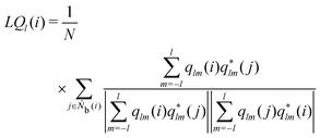 | (33) |
| |  | (34) |
| |  | (35) |
The locally averaged alternative bond-orientational order parameters
![[L with combining macron]](https://www.rsc.org/images/entities/i_char_004c_0304.gif) Q
Q and
![[L with combining macron]](https://www.rsc.org/images/entities/i_char_004c_0304.gif) W
W are defined as
| |  | (36) |
| |  | (37) |
The modified alternative bond-orientational order parameters LQM and LWM, locally averaged over the lqlm of LQ and LW, were implemented in MALIO. LQM and LWM are expressed as
| | 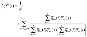 | (38) |
| |  | (39) |
| |  | (40) |
The locally averaged modified alternative bond-orientational order parameters
![[L with combining macron]](https://www.rsc.org/images/entities/i_char_004c_0304.gif) QM
QM and
![[L with combining macron]](https://www.rsc.org/images/entities/i_char_004c_0304.gif) WM
WM are defined as
| |  | (41) |
| |  | (42) |
The Legendre polynomial parameter S considered in this work is expressed as
| |  | (43) |
where
Pn is an
n-th order Legendre polynomial function, and
u is a unit direction vector.
S is inspired by Onsager's order parameter,
68 but the molecular system average of
S does not match Onsager's order parameter because the orientation direction of particle
i is used instead of the average orientation direction. Note that
S2 is used to observe the isotropic-nematic transition of uniaxial liquid crystals.
55 We consider
n = 2, 4, and 6. The locally averaged Legendre polynomial parameter
![[S with combining macron]](https://www.rsc.org/images/entities/i_char_0053_0304.gif)
is defined as
| |  | (44) |
The modified Legendre polynomial parameter T in this work is expressed as
| |  | (45) |
where
z is the distance from particle
j to the plane perpendicular to the orientation direction of particle
i containing the coordinates of particle
i, and the parameter
d is the distance between parallel layered structures.
T is inspired by MacMillan's smectic order parameter,
69 but the molecular system average of
T does not match MacMillan's order parameter because the orientation direction of particle
i is used instead of the average orientation direction. We consider
d = 2.0, 2.25, 2.5, 2.75, 3.0, 3.25, 3.5, and 3.75. The locally averaged Legendre polynomial parameter
![[T with combining macron]](https://www.rsc.org/images/entities/i_char_0054_0304.gif)
is defined as
| |  | (46) |
Because actual neighbors such as Nb(i) and Nb(i,j) directly influence the LOP values, their selection is an important factor in extracting local molecular structures. Several protocols are possible, such as using particles within the cutoff radius as neighbors,26,35,42,45–48 predetermining the number of neighboring particles,32,42,45–48 and using Delaunay triangulation based on Voronoi diagrams.48,51,70,71 All of the above protocols are implemented in MALIO, and can be selected according to the molecular structure characteristics and the correspondence with various additional analyses after the LOP values are determined. In this work, the number of neighboring particles was fixed on the basis of previous studies32,45 on liquid crystal molecules. Specifically, N was varied from 6 to 14, and the optimal LOP for each N was searched.
In addition to single LOPs, the classification performances of combinations of two LOPs were also evaluated. Therefore, a total of 2![[thin space (1/6-em)]](https://www.rsc.org/images/entities/char_2009.gif) 220
220![[thin space (1/6-em)]](https://www.rsc.org/images/entities/char_2009.gif) 777 (=(702C1 + 702C2) × 9 neighboring conditions) different combinations of LOPs were considered.
777 (=(702C1 + 702C2) × 9 neighboring conditions) different combinations of LOPs were considered.
2.3 Machine learning strategy for screening LOPs
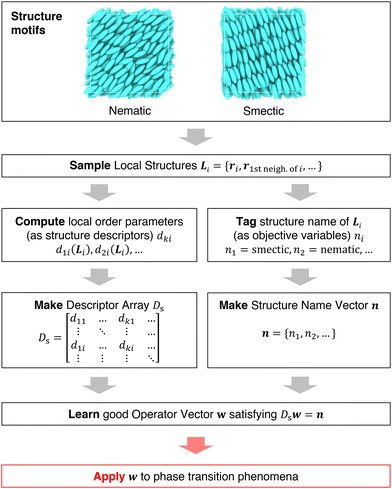
It is difficult to examine in detail the ability to extract the local molecular structure in transition for more than 2 million LOP combinations, even with the high efficiency of machine learning. Therefore, MALIO screens LOPs according to the most important and simple question: Can LOPs successfully distinguish between pre- and post-transition molecular structures? This is because, at minimum, good LOPs must be able to distinguish between pre- and post-transition molecular structures with high accuracy to enable comprehensive observation of events during transition. The procedure for performing the above screening is shown in Fig. 1: (i) first, small nematic and smectic molecular structures were entered into MALIO to serve as motifs for the molecular systems before and after the transition. The input structures were created in the same manner as described in the subsection “Molecular Dynamics Simulations”, but the number of molecules was set to 1701, which is small enough to create well-defined molecular structures. The number of input structures was set to 200 for each of the two structures. (ii) MALIO extracted each SCGB particle and its neighboring particles from each molecular structure using the neighboring protocol and determined the local particle coordinates Li. Here, we chose the protocol in which the number of neighboring particles is predetermined. That is, Li represents the information on particle i and the nearest to N-th nearest neighbor from particle i. (iii) Structural descriptors were determined by calculating 702 LOPs for all 680![[thin space (1/6-em)]](https://www.rsc.org/images/entities/char_2009.gif) 400 (= 1701 particles × 200 coordinate data × 2 phases) of Lis. The structure name (nematic or smectic) was tagged onto each Li and designated as the objective variable. (iv) The structure descriptors and objective variables were then stored in the descriptor array Ds and the structure name vector n, respectively. (v) Finally, the random forest method implemented in Scikit-learn (version 0.20.3)72 was used to estimate the operator vector w satisfying the relation Dsw = n. The number of trees in the forest was set to 100, and the maximum depth of each tree was set to 10. Default values in Scikit-learn were used for the other settings. The quality of w was also checked by 5-fold cross-validation implemented in Scikit-learn. The combination of two LOPs can be considered by arbitrarily selecting two of the elements of w and setting the others to null. This process was carried out using a sequential forward selection algorithm.73 The classification accuracy of each (set of) LOP(s) was calculated from the correct tagging rate (CTR) as implemented in MALIO. The CTR c is defined as
400 (= 1701 particles × 200 coordinate data × 2 phases) of Lis. The structure name (nematic or smectic) was tagged onto each Li and designated as the objective variable. (iv) The structure descriptors and objective variables were then stored in the descriptor array Ds and the structure name vector n, respectively. (v) Finally, the random forest method implemented in Scikit-learn (version 0.20.3)72 was used to estimate the operator vector w satisfying the relation Dsw = n. The number of trees in the forest was set to 100, and the maximum depth of each tree was set to 10. Default values in Scikit-learn were used for the other settings. The quality of w was also checked by 5-fold cross-validation implemented in Scikit-learn. The combination of two LOPs can be considered by arbitrarily selecting two of the elements of w and setting the others to null. This process was carried out using a sequential forward selection algorithm.73 The classification accuracy of each (set of) LOP(s) was calculated from the correct tagging rate (CTR) as implemented in MALIO. The CTR c is defined as| |  | (47) |
where Zcorrect is the number of correct tags obtained from Dsw, and Ztotal is the total number of tags. LOPs were screened using the CTR. The (set of) LOP(s) that performed best (i.e., the maximum value of c) for each N was finally selected.
 |
| | Fig. 1 Screening steps. | |
2.4 Application of selected LOPs to the nematic–smectic transition
Once the candidate LOPs were carefully selected using the screening strategy, the LOPs were applied to observe the nematic–smectic phase transition. The following procedure was implemented: (i) candidate LOPs were calculated for the time evolution of the three-dimensional coordinate data of a molecular system in which a monodomain nematic phase with 1 million SCGB particles was quenched to the temperature at which it becomes smectic (temperature T = 1.8; see the subsection “Molecular Dynamics Simulations”). (ii) The values of the specific (set of) LOP(s) were stored in the descriptor array Ds,q. The elements of Ds,q corresponding to other LOPs were set to null. Here, Ds,q is a function of time corresponding to the coordinates at each time. (iii) We estimated whether each particle belonged to the nematic- or smectic-like structure by applying w from the previous subsection to Ds,q (the elements other than the candidate LOPs were set to null). Note that w is an operator vector learned from small nematic and smectic molecular structures and is independent of time. (iv) A cluster analysis was performed for the smectic molecules on the basis of the structure name tagged onto each particle at each time point. In this case, the neighboring conditions used as criteria for particle grouping were identical to those of the LOP neighboring protocol. The above procedure was used to obtain the kinetics of the phase transition phenomena, including nucleation and subsequent percolation, in the form of cluster statistics. The obtained results were compared to examine the influence of the choice of LOP species and neighboring particles on the cluster statistics.
3 Results and discussion
3.1 Evaluation of MALIO's ability to compute local order parameters
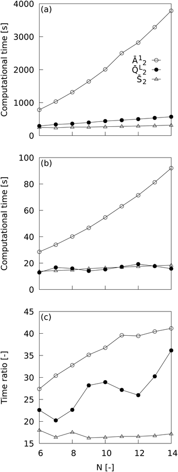
MALIO is a package that is an advanced version of ML-LSA with complete re-coding in Cython and improvements in related libraries, and is expected to speed up LOP computation, but it should be quantitatively demonstrated how much speedup is actually achieved. Fig. 2 shows the dependence of LOP computational time on the number of neighboring particles when using (a) ML-LSA and (b) MALIO; the ratio of LOP computational time for ML-LSA to that for MALIO is also plotted in (c). One core of Intel(R) Xeon(R) Gold 6252 CPU @ 2.10 GHz was used to measure the LOP computation time. The LOP computation time plotted in Fig. 2 was measured at the end of the LOP computation for 680,400 of Lis. Ā12 is the LOP with relatively high computational cost, ![[Q with combining macron]](https://www.rsc.org/images/entities/i_char_0051_0304.gif) L2 is the LOP calculated by MALIO's original spherical harmonic function library, and
L2 is the LOP calculated by MALIO's original spherical harmonic function library, and ![[S with combining macron]](https://www.rsc.org/images/entities/i_char_0053_0304.gif) 2 is the LOP with relatively low computational cost. In ML-LSA, the computational time for Ā12 and
2 is the LOP with relatively low computational cost. In ML-LSA, the computational time for Ā12 and ![[Q with combining macron]](https://www.rsc.org/images/entities/i_char_0051_0304.gif) L2 increased with increasing N, while the computational time for
L2 increased with increasing N, while the computational time for ![[S with combining macron]](https://www.rsc.org/images/entities/i_char_0053_0304.gif) 2 hardly increased with increasing N. In MALIO, the computational time was much shorter than in ML-LSA. The computational time for Ā12 increased with increasing N, while the computational time for
2 hardly increased with increasing N. In MALIO, the computational time was much shorter than in ML-LSA. The computational time for Ā12 increased with increasing N, while the computational time for ![[Q with combining macron]](https://www.rsc.org/images/entities/i_char_0051_0304.gif) L2 and
L2 and ![[S with combining macron]](https://www.rsc.org/images/entities/i_char_0053_0304.gif) 2 hardly increased with increasing N. Efficient computation of
2 hardly increased with increasing N. Efficient computation of ![[Q with combining macron]](https://www.rsc.org/images/entities/i_char_0051_0304.gif) L2 by MALIO's original spherical harmonic function calculation library resulted in saturation of
L2 by MALIO's original spherical harmonic function calculation library resulted in saturation of ![[Q with combining macron]](https://www.rsc.org/images/entities/i_char_0051_0304.gif) L2 computational time with respect to N. The ratio of LOP computational time for ML-LSA to that for MALIO reveals a dramatic speedup in LOP computational time with MALIO. A maximum speedup of over 40 times was achieved in Ā12, and a maximum speedup of over 35 times was achieved in
L2 computational time with respect to N. The ratio of LOP computational time for ML-LSA to that for MALIO reveals a dramatic speedup in LOP computational time with MALIO. A maximum speedup of over 40 times was achieved in Ā12, and a maximum speedup of over 35 times was achieved in ![[Q with combining macron]](https://www.rsc.org/images/entities/i_char_0051_0304.gif) L2. Even in
L2. Even in ![[S with combining macron]](https://www.rsc.org/images/entities/i_char_0053_0304.gif) 2, where the computational cost is relatively low, a speedup of over 17 times was achieved.
2, where the computational cost is relatively low, a speedup of over 17 times was achieved.
 |
| | Fig. 2 Dependence of LOP computational time on the number of neighboring particles when using (a) ML-LSA and (b) MALIO. The ratio of LOP computational time for ML-LSA to that for MALIO is also plotted in (c). | |
3.2 Screening of local order parameters
Table 2 shows the (set of) LOP(s) that best distinguished nematic and smectic phases. The second- and third-best (sets of) LOPs are also shown. The ![[Q with combining macron]](https://www.rsc.org/images/entities/i_char_0051_0304.gif) L series was found to be the best single LOP for all N conditions. In particular,
L series was found to be the best single LOP for all N conditions. In particular, ![[Q with combining macron]](https://www.rsc.org/images/entities/i_char_0051_0304.gif) L2 attained the best CTR for N ≥ 8 and was the most robust to N. The best set of two LOPs was also found to be the combination of the
L2 attained the best CTR for N ≥ 8 and was the most robust to N. The best set of two LOPs was also found to be the combination of the ![[Q with combining macron]](https://www.rsc.org/images/entities/i_char_0051_0304.gif) L series (chosen as the best single LOP) and the QL series for all N conditions. However, the improvement in c due to adding the QL series was small (less than 0.01 for almost all N), and the increase in the number of LOPs was not commensurate with the CTR increase. Recall that in additional analyses such as drawing free energy landscapes, increasing the number of LOPs leads directly to an exponential increase in computational cost due to the curse of dimensionality, and makes it less easy to interpret results. A single LOP should be used in the above cases. The second- and third-best LOPs also fall into this case.
L series (chosen as the best single LOP) and the QL series for all N conditions. However, the improvement in c due to adding the QL series was small (less than 0.01 for almost all N), and the increase in the number of LOPs was not commensurate with the CTR increase. Recall that in additional analyses such as drawing free energy landscapes, increasing the number of LOPs leads directly to an exponential increase in computational cost due to the curse of dimensionality, and makes it less easy to interpret results. A single LOP should be used in the above cases. The second- and third-best LOPs also fall into this case.
Table 2 Peak performance of each (set of) LOP(s) in distinguishing nematic and smectic structures. LOP is an abbreviation for local order parameter and CTR is an abbreviation for correct tagging rate
|
N [–] |
LOP (CTR [–]) |
| Best |
Second-best |
Third-best |
| 6 |
![[Q with combining macron]](https://www.rsc.org/images/entities/i_char_0051_0304.gif) L6 (0.978 ± 0.004)
L6 (0.978 ± 0.004) |
Ā
12 (0.955 ± 0.006) |
Q
L6 (0.954 ± 0.004) |
| 7 |
![[Q with combining macron]](https://www.rsc.org/images/entities/i_char_0051_0304.gif) L6 (0.977 ± 0.004)
L6 (0.977 ± 0.004) |
![[Q with combining macron]](https://www.rsc.org/images/entities/i_char_0051_0304.gif) L2 (0.959 ± 0.008)
L2 (0.959 ± 0.008) |
Ā
12 (0.958 ± 0.007) |
| 8 |
![[Q with combining macron]](https://www.rsc.org/images/entities/i_char_0051_0304.gif) L2 (0.976 ± 0.005)
L2 (0.976 ± 0.005) |
![[Q with combining macron]](https://www.rsc.org/images/entities/i_char_0051_0304.gif) L12 (0.974 ± 0.004)
L12 (0.974 ± 0.004) |
![[Q with combining macron]](https://www.rsc.org/images/entities/i_char_0051_0304.gif) L6 (0.969 ± 0.004)
L6 (0.969 ± 0.004) |
| 9 |
![[Q with combining macron]](https://www.rsc.org/images/entities/i_char_0051_0304.gif) L2 (0.985 ± 0.004)
L2 (0.985 ± 0.004) |
![[Q with combining macron]](https://www.rsc.org/images/entities/i_char_0051_0304.gif) L12 (0.982 ± 0.004)
L12 (0.982 ± 0.004) |
![[F with combining macron]](https://www.rsc.org/images/entities/i_char_0046_0304.gif) f
3,f3,6.0 (0.973 ± 0.004)
f
3,f3,6.0 (0.973 ± 0.004) |
| 10 |
![[Q with combining macron]](https://www.rsc.org/images/entities/i_char_0051_0304.gif) L2 (0.991 ± 0.003)
L2 (0.991 ± 0.003) |
![[Q with combining macron]](https://www.rsc.org/images/entities/i_char_0051_0304.gif) L12 (0.987 ± 0.003)
L12 (0.987 ± 0.003) |
Ā
12 (0.978 ± 0.006) |
| 11 |
![[Q with combining macron]](https://www.rsc.org/images/entities/i_char_0051_0304.gif) L2 (0.994 ± 0.002)
L2 (0.994 ± 0.002) |
![[Q with combining macron]](https://www.rsc.org/images/entities/i_char_0051_0304.gif) L12 (0.990 ± 0.003)
L12 (0.990 ± 0.003) |
Ā
12 (0.982 ± 0.005) |
| 12 |
![[Q with combining macron]](https://www.rsc.org/images/entities/i_char_0051_0304.gif) L2 (0.996 ± 0.001)
L2 (0.996 ± 0.001) |
![[Q with combining macron]](https://www.rsc.org/images/entities/i_char_0051_0304.gif) L12 (0.992 ± 0.002)
L12 (0.992 ± 0.002) |
Ā
12 (0.984 ± 0.005) |
| 13 |
![[Q with combining macron]](https://www.rsc.org/images/entities/i_char_0051_0304.gif) L2 (0.997 ± 0.001)
L2 (0.997 ± 0.001) |
![[Q with combining macron]](https://www.rsc.org/images/entities/i_char_0051_0304.gif) L12 (0.994 ± 0.002)
L12 (0.994 ± 0.002) |
![[B with combining macron]](https://www.rsc.org/images/entities/i_char_0042_0304.gif) 1,3,π/6 (0.988 ± 0.004)
1,3,π/6 (0.988 ± 0.004) |
| 14 |
![[Q with combining macron]](https://www.rsc.org/images/entities/i_char_0051_0304.gif) L2 (0.998 ± 0.001)
L2 (0.998 ± 0.001) |
![[Q with combining macron]](https://www.rsc.org/images/entities/i_char_0051_0304.gif) L12 (0.995 ± 0.002)
L12 (0.995 ± 0.002) |
![[B with combining macron]](https://www.rsc.org/images/entities/i_char_0042_0304.gif) 1,3,π/6 (0.991 ± 0.004)
1,3,π/6 (0.991 ± 0.004) |
| 6 |
{![[Q with combining macron]](https://www.rsc.org/images/entities/i_char_0051_0304.gif) L6,QL6} (0.988 ± 0.003) L6,QL6} (0.988 ± 0.003) |
{Ā12,![[Q with combining macron]](https://www.rsc.org/images/entities/i_char_0051_0304.gif) L5} (0.968 ± 0.006) L5} (0.968 ± 0.006) |
{QL6,![[Q with combining macron]](https://www.rsc.org/images/entities/i_char_0051_0304.gif) L5} (0.967 ± 0.005) L5} (0.967 ± 0.005) |
| 7 |
{![[Q with combining macron]](https://www.rsc.org/images/entities/i_char_0051_0304.gif) L6,QL6} (0.986 ± 0.003) L6,QL6} (0.986 ± 0.003) |
{![[Q with combining macron]](https://www.rsc.org/images/entities/i_char_0051_0304.gif) L2, L2,![[Q with combining macron]](https://www.rsc.org/images/entities/i_char_0051_0304.gif) L12} (0.981 ± 0.004) L12} (0.981 ± 0.004) |
{Ā12,![[Q with combining macron]](https://www.rsc.org/images/entities/i_char_0051_0304.gif) L12} (0.976 ± 0.005) L12} (0.976 ± 0.005) |
| 8 |
{![[Q with combining macron]](https://www.rsc.org/images/entities/i_char_0051_0304.gif) L2,QL2} (0.989 ± 0.003) L2,QL2} (0.989 ± 0.003) |
{![[Q with combining macron]](https://www.rsc.org/images/entities/i_char_0051_0304.gif) L12, L12,![[Q with combining macron]](https://www.rsc.org/images/entities/i_char_0051_0304.gif) L4} (0.984 ± 0.004) L4} (0.984 ± 0.004) |
{![[Q with combining macron]](https://www.rsc.org/images/entities/i_char_0051_0304.gif) L6, L6,![[B with combining macron]](https://www.rsc.org/images/entities/i_char_0042_0304.gif) 1,1,π/4} (0.981 ± 0.004) 1,1,π/4} (0.981 ± 0.004) |
| 9 |
{![[Q with combining macron]](https://www.rsc.org/images/entities/i_char_0051_0304.gif) L2,QL2} (0.994 ± 0.002) L2,QL2} (0.994 ± 0.002) |
{![[Q with combining macron]](https://www.rsc.org/images/entities/i_char_0051_0304.gif) L12, L12,![[Q with combining macron]](https://www.rsc.org/images/entities/i_char_0051_0304.gif) L4} (0.990 ± 0.003) L4} (0.990 ± 0.003) |
{![[F with combining macron]](https://www.rsc.org/images/entities/i_char_0046_0304.gif) f3,f2,6.0, f3,f2,6.0,![[S with combining macron]](https://www.rsc.org/images/entities/i_char_0053_0304.gif) 2} (0.983 ± 0.003) 2} (0.983 ± 0.003) |
| 10 |
{![[Q with combining macron]](https://www.rsc.org/images/entities/i_char_0051_0304.gif) L2,QL2} (0.997 ± 0.001) L2,QL2} (0.997 ± 0.001) |
{![[Q with combining macron]](https://www.rsc.org/images/entities/i_char_0051_0304.gif) L12,QL12} (0.993 ± 0.002) L12,QL12} (0.993 ± 0.002) |
{Ā12,![[W with combining macron]](https://www.rsc.org/images/entities/i_char_0057_0304.gif) L2} (0.985 ± 0.004) L2} (0.985 ± 0.004) |
| 11 |
{![[Q with combining macron]](https://www.rsc.org/images/entities/i_char_0051_0304.gif) L2,QL2} (0.998 ± 0.001) L2,QL2} (0.998 ± 0.001) |
{![[Q with combining macron]](https://www.rsc.org/images/entities/i_char_0051_0304.gif) L12,QL12} (0.995 ± 0.002) L12,QL12} (0.995 ± 0.002) |
{Ā12,![[W with combining macron]](https://www.rsc.org/images/entities/i_char_0057_0304.gif) L2} (0.988 ± 0.004) L2} (0.988 ± 0.004) |
| 12 |
{![[Q with combining macron]](https://www.rsc.org/images/entities/i_char_0051_0304.gif) L2,QL2} (0.999 ± 0.001) L2,QL2} (0.999 ± 0.001) |
{![[Q with combining macron]](https://www.rsc.org/images/entities/i_char_0051_0304.gif) L12,QL12} (0.997 ± 0.001) L12,QL12} (0.997 ± 0.001) |
{Ā12,![[W with combining macron]](https://www.rsc.org/images/entities/i_char_0057_0304.gif) L2} (0.990 ± 0.004) L2} (0.990 ± 0.004) |
| 13 |
{![[Q with combining macron]](https://www.rsc.org/images/entities/i_char_0051_0304.gif) L2,QL2} (1.000 ± 0.000) L2,QL2} (1.000 ± 0.000) |
{![[Q with combining macron]](https://www.rsc.org/images/entities/i_char_0051_0304.gif) L12,QL12} (0.998 ± 0.001) L12,QL12} (0.998 ± 0.001) |
{![[B with combining macron]](https://www.rsc.org/images/entities/i_char_0042_0304.gif) 1,3,π/6, 1,3,π/6,![[W with combining macron]](https://www.rsc.org/images/entities/i_char_0057_0304.gif) L2} (0.994 ± 0.003) L2} (0.994 ± 0.003) |
| 14 |
{![[Q with combining macron]](https://www.rsc.org/images/entities/i_char_0051_0304.gif) L2,QL2} (1.000 ± 0.000) L2,QL2} (1.000 ± 0.000) |
{![[Q with combining macron]](https://www.rsc.org/images/entities/i_char_0051_0304.gif) L12,QL12} (0.998 ± 0.001) L12,QL12} (0.998 ± 0.001) |
{![[B with combining macron]](https://www.rsc.org/images/entities/i_char_0042_0304.gif) 1,3,π/6, 1,3,π/6,![[W with combining macron]](https://www.rsc.org/images/entities/i_char_0057_0304.gif) L2} (0.996 ± 0.002) L2} (0.996 ± 0.002) |
The local average was used for almost all of the single LOPs from best to third-best. Therefore, to explore other possibilities for the two LOP sets, we examined the CTRs only for LOPs that were not locally averaged. Table 3 shows the (set of) LOP(s) that best distinguished nematic and smectic phases when the locally averaged LOPs were excluded. At 8 ≤ N ≤ 11, the best LOP set was the combination of QL2 and QL12. Considering both high CTR and robustness to N, subsequent analyses were performed for ![[Q with combining macron]](https://www.rsc.org/images/entities/i_char_0051_0304.gif) L6,
L6, ![[Q with combining macron]](https://www.rsc.org/images/entities/i_char_0051_0304.gif) L2,
L2, ![[Q with combining macron]](https://www.rsc.org/images/entities/i_char_0051_0304.gif) L12, Ā12, {QL2,QL12}, QL2, and QL12.
L12, Ā12, {QL2,QL12}, QL2, and QL12.
Table 3 Peak performance of each (set of) locally unaveraged LOP(s) in distinguishing between nematic and smectic structures. LOP is an abbreviation for local order parameter and CTR is an abbreviation for correct tagging rate
|
N [–] |
LOP |
CTR [—] |
| 6 |
Q
L6
|
0.954 ± 0.004 |
| 7 |
Q
L6
|
0.945 ± 0.004 |
| 8 |
Q
L12
|
0.938 ± 0.003 |
| 9 |
Q
L12
|
0.954 ± 0.004 |
| 10 |
Q
L2
|
0.965 ± 0.007 |
| 11 |
Q
L2
|
0.973 ± 0.006 |
| 12 |
Q
L2
|
0.979 ± 0.005 |
| 13 |
H
1.0
|
0.984 ± 0.005 |
| 14 |
H
1.0
|
0.989 ± 0.004 |
| 6 |
{QL6,B2,3,π/2} |
0.958 ± 0.005 |
| 7 |
{QL6,QL2} |
0.957 ± 0.005 |
| 8 |
{QL12,QL2} |
0.965 ± 0.005 |
| 9 |
{QL12,QL2} |
0.976 ± 0.005 |
| 10 |
{QL2,QL12} |
0.982 ± 0.004 |
| 11 |
{QL2,QL12} |
0.987 ± 0.004 |
| 12 |
{QL2,H6.0} |
0.990 ± 0.003 |
| 13 |
{H1.0,H6.0} |
0.992 ± 0.003 |
| 14 |
{H1.0,H6.0} |
0.994 ± 0.003 |
3.3 Impact of a small number of neighboring particles
As long as the LOP can distinguish local structures in transition with high accuracy, it is desirable to have as few neighboring particles as possible. For a small number of neighboring particles (N = 6 and 7), ![[Q with combining macron]](https://www.rsc.org/images/entities/i_char_0051_0304.gif) L6 is the best LOP. Therefore, we first observed the cluster statistics when
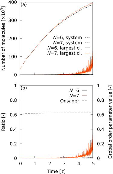
L6 is the best LOP. Therefore, we first observed the cluster statistics when ![[Q with combining macron]](https://www.rsc.org/images/entities/i_char_0051_0304.gif) L6 was used. Fig. 3 shows (a) the time evolution of the number of smectic molecules in the system and in the maximum cluster, and (b) the ratio of the number of molecules in the largest cluster to the number of smectic molecules in the system. The time evolution of Onsager's global order parameter was also plotted in Fig. 3(b). With the CTR of
L6 was used. Fig. 3 shows (a) the time evolution of the number of smectic molecules in the system and in the maximum cluster, and (b) the ratio of the number of molecules in the largest cluster to the number of smectic molecules in the system. The time evolution of Onsager's global order parameter was also plotted in Fig. 3(b). With the CTR of ![[Q with combining macron]](https://www.rsc.org/images/entities/i_char_0051_0304.gif) L6 for N = 6 and 7 (c ∼ 0.98), a number of smectic molecules were detected even in the initial structure, which should be completely in the nematic phase. This depends completely on the CTRs in Table 2, implying that extremely high CTRs are required to observe cluster statistics in nucleation. At t = 5.0 τ, the total number of smectic molecules reached about 400
L6 for N = 6 and 7 (c ∼ 0.98), a number of smectic molecules were detected even in the initial structure, which should be completely in the nematic phase. This depends completely on the CTRs in Table 2, implying that extremely high CTRs are required to observe cluster statistics in nucleation. At t = 5.0 τ, the total number of smectic molecules reached about 400![[thin space (1/6-em)]](https://www.rsc.org/images/entities/char_2009.gif) 000. However, it is clear from Fig. 3(b) that the largest cluster did not grow at all until t = 5.0 τ. The results indicate that the transition does not progress from nucleation to percolation, even though approximately 40% of the molecules are determined to be smectic molecules. The same trend was observed for other LOP species when N = 6 and 7 were used (data not shown). This unnatural behavior indicates that N is too small and is insufficient to capture the smectic layer. Therefore, in the following analysis, the conditions N = 8–14 were used and
000. However, it is clear from Fig. 3(b) that the largest cluster did not grow at all until t = 5.0 τ. The results indicate that the transition does not progress from nucleation to percolation, even though approximately 40% of the molecules are determined to be smectic molecules. The same trend was observed for other LOP species when N = 6 and 7 were used (data not shown). This unnatural behavior indicates that N is too small and is insufficient to capture the smectic layer. Therefore, in the following analysis, the conditions N = 8–14 were used and ![[Q with combining macron]](https://www.rsc.org/images/entities/i_char_0051_0304.gif) L6 was excluded. Note that Onsager's global order parameter was also insensitive to increases in the number of smectic molecules.
L6 was excluded. Note that Onsager's global order parameter was also insensitive to increases in the number of smectic molecules.
 |
| | Fig. 3 (a) Time evolution of the number of smectic molecules in the system and in the maximum cluster. (b) Ratio of the number of molecules in the largest cluster to the number of smectic molecules in the system. The time evolution of Onsager's global order parameter was also plotted. | |
3.4 Pre-nucleation behavior
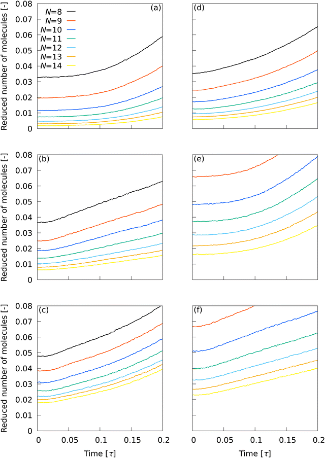
The behavior of the number of smectic molecules in the system at the beginning of the transition is important because it affects the subsequent nucleation process. Fig. 4 shows the time evolution of the number of smectic molecules at 0 ≤ t ≤ 0.2τ in the system observed using (a) ![[Q with combining macron]](https://www.rsc.org/images/entities/i_char_0051_0304.gif) L2, (b)
L2, (b) ![[Q with combining macron]](https://www.rsc.org/images/entities/i_char_0051_0304.gif) L12, (c) Ā12, (d) {QL2,QL12}, (e) QL2, and (f) QL12. The number of smectic molecules was divided by the total number of molecules. The initially observed smectic molecules originate from the error in classification using LOPs. With
L12, (c) Ā12, (d) {QL2,QL12}, (e) QL2, and (f) QL12. The number of smectic molecules was divided by the total number of molecules. The initially observed smectic molecules originate from the error in classification using LOPs. With ![[Q with combining macron]](https://www.rsc.org/images/entities/i_char_0051_0304.gif) L2, the number of initial smectic molecules could be suppressed to less than 0.5% for N ≥ 12. That the number of molecules hardly increased with time up to t > 0.1τ independently of N is consistent with the fact that cluster formation is less likely to proceed in the initial nucleation stage.
L2, the number of initial smectic molecules could be suppressed to less than 0.5% for N ≥ 12. That the number of molecules hardly increased with time up to t > 0.1τ independently of N is consistent with the fact that cluster formation is less likely to proceed in the initial nucleation stage.
 |
| | Fig. 4 Time evolution of the number of smectic molecules at 0 ≤ t ≤ 0.2τ in the system observed using (a) ![[Q with combining macron]](https://www.rsc.org/images/entities/i_char_0051_0304.gif) L2, (b) L2, (b) ![[Q with combining macron]](https://www.rsc.org/images/entities/i_char_0051_0304.gif) L12, (c) Ā12, (d) {QL2,QL12}, (e) QL2, and (f) QL12. The number of smectic molecules was divided by the total number of molecules. L12, (c) Ā12, (d) {QL2,QL12}, (e) QL2, and (f) QL12. The number of smectic molecules was divided by the total number of molecules. | |
With ![[Q with combining macron]](https://www.rsc.org/images/entities/i_char_0051_0304.gif) L12, the number of initial smectic molecules could be suppressed to less than 1% for N ≥ 13, but the observed number of smectic molecules increased immediately afterwards. With Ā12, the number of initial smectic molecules could not be suppressed to less than 1% for any of the N conditions, nor could the increase in the number of smectic molecules immediately afterwards be suppressed. With {QL2,QL12}, the number of initial smectic molecules could be suppressed to less than 1% for N ≥ 12, but the number of smectic molecules increased immediately afterwards. With QL2, the number of initial smectic molecules could not be suppressed to less than 1% for any of the N conditions, but its increase with time at t > 0.1τ was similar to that for
L12, the number of initial smectic molecules could be suppressed to less than 1% for N ≥ 13, but the observed number of smectic molecules increased immediately afterwards. With Ā12, the number of initial smectic molecules could not be suppressed to less than 1% for any of the N conditions, nor could the increase in the number of smectic molecules immediately afterwards be suppressed. With {QL2,QL12}, the number of initial smectic molecules could be suppressed to less than 1% for N ≥ 12, but the number of smectic molecules increased immediately afterwards. With QL2, the number of initial smectic molecules could not be suppressed to less than 1% for any of the N conditions, but its increase with time at t > 0.1τ was similar to that for ![[Q with combining macron]](https://www.rsc.org/images/entities/i_char_0051_0304.gif) L2. With QL12, the number of initial smectic molecules could not be suppressed to less than 1% for any of the N conditions, nor could the increase in number of smectic molecules immediately afterwards be suppressed. The results indicate the superiority of
L2. With QL12, the number of initial smectic molecules could not be suppressed to less than 1% for any of the N conditions, nor could the increase in number of smectic molecules immediately afterwards be suppressed. The results indicate the superiority of ![[Q with combining macron]](https://www.rsc.org/images/entities/i_char_0051_0304.gif) L2.
L2.
3.5 Percolation transition
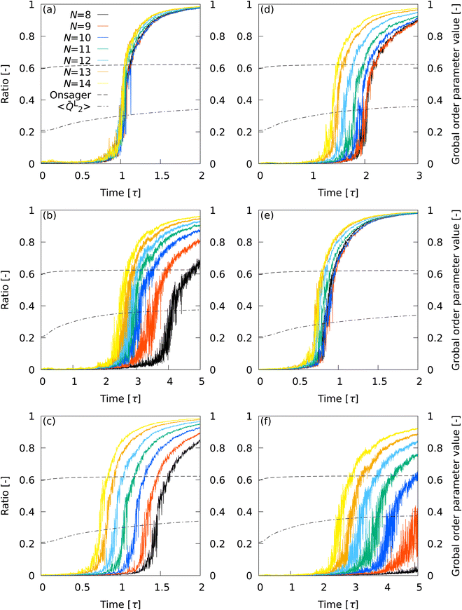
The progress from nucleation to percolation is also noteworthy. Fig. 5 shows the time evolution of the ratio of the number of smectic molecules in the largest cluster to the number of smectic molecules in the system, captured by (a) ![[Q with combining macron]](https://www.rsc.org/images/entities/i_char_0051_0304.gif) L2, (b)
L2, (b) ![[Q with combining macron]](https://www.rsc.org/images/entities/i_char_0051_0304.gif) L12, (c) Ā12, (d) {QL2,QL12}, (e) QL2, and (f) QL12. The Onsager's order parameter and the all-particle mean of
L12, (c) Ā12, (d) {QL2,QL12}, (e) QL2, and (f) QL12. The Onsager's order parameter and the all-particle mean of ![[Q with combining macron]](https://www.rsc.org/images/entities/i_char_0051_0304.gif) L2, 〈
L2, 〈![[Q with combining macron]](https://www.rsc.org/images/entities/i_char_0051_0304.gif) L2〉, were also plotted to show the time evolution of global order parameters. A rapid increase in the ratio signifies the onset of percolation, and the onset of convergence to 1 signifies completion of percolation. With
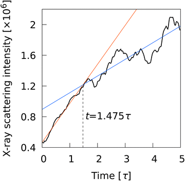
L2〉, were also plotted to show the time evolution of global order parameters. A rapid increase in the ratio signifies the onset of percolation, and the onset of convergence to 1 signifies completion of percolation. With ![[Q with combining macron]](https://www.rsc.org/images/entities/i_char_0051_0304.gif) L2, the curves overlapped for all N conditions, indicating that the percolation onset and completion times were independent of N. The completion time (t ∼ 1.5τ) agreed perfectly with the results of numerical analysis corresponding to X-ray scattering experiments on liquid crystal molecular systems undergoing phase transition. Fig. 6 shows the time evolution of X-ray scattering intensity calculated for the liquid crystal molecular systems during the phase transition. The time evolution of scattering intensity was calculated using the following procedure: (i) the scattering pattern at each time was calculated on the basis of previous studies.74,75 (ii) Because the intensity difference between the two phases is larger near the second harmonic according to previous studies,32,74,75 the intensity at each time was integrated over a rectangular region cut in the ranges −3.5σ−1 ≤ qa ≤ 3.5σ−1 and 3.5σ−1 ≤ qb ≤ 6.0σ−1, where qa and qb are the wavenumbers of the components perpendicular and parallel to the liquid crystal orientation direction, respectively. Because the X-ray analysis is performed completely independently from the various analyses using LOPs, it can be used as one indicator to evaluate LOP performance. The X-ray intensity increased almost linearly for 0 ≤ t ≤ 1.475τ. However, for t > 1.475τ, the increasing trend became gradual and intermittent. The results show that the smectic local structures complete percolation at t = 1.475τ, implying the number of smectic molecules in the largest cluster becomes almost equal to the number of total smectic molecules in the system.
L2, the curves overlapped for all N conditions, indicating that the percolation onset and completion times were independent of N. The completion time (t ∼ 1.5τ) agreed perfectly with the results of numerical analysis corresponding to X-ray scattering experiments on liquid crystal molecular systems undergoing phase transition. Fig. 6 shows the time evolution of X-ray scattering intensity calculated for the liquid crystal molecular systems during the phase transition. The time evolution of scattering intensity was calculated using the following procedure: (i) the scattering pattern at each time was calculated on the basis of previous studies.74,75 (ii) Because the intensity difference between the two phases is larger near the second harmonic according to previous studies,32,74,75 the intensity at each time was integrated over a rectangular region cut in the ranges −3.5σ−1 ≤ qa ≤ 3.5σ−1 and 3.5σ−1 ≤ qb ≤ 6.0σ−1, where qa and qb are the wavenumbers of the components perpendicular and parallel to the liquid crystal orientation direction, respectively. Because the X-ray analysis is performed completely independently from the various analyses using LOPs, it can be used as one indicator to evaluate LOP performance. The X-ray intensity increased almost linearly for 0 ≤ t ≤ 1.475τ. However, for t > 1.475τ, the increasing trend became gradual and intermittent. The results show that the smectic local structures complete percolation at t = 1.475τ, implying the number of smectic molecules in the largest cluster becomes almost equal to the number of total smectic molecules in the system.
 |
| | Fig. 5 Time evolution of the ratio of the number of smectic molecules in the largest cluster to the number of smectic molecules in the system, captured by (a) ![[Q with combining macron]](https://www.rsc.org/images/entities/i_char_0051_0304.gif) L2, (b) L2, (b) ![[Q with combining macron]](https://www.rsc.org/images/entities/i_char_0051_0304.gif) L12, (c) Ā12, (d) {QL2,QL12}, (e) QL2, and (f) QL12. The Onsager's order parameter and 〈 L12, (c) Ā12, (d) {QL2,QL12}, (e) QL2, and (f) QL12. The Onsager's order parameter and 〈![[Q with combining macron]](https://www.rsc.org/images/entities/i_char_0051_0304.gif) L2〉 were also plotted to show the time evolution of global order parameters. L2〉 were also plotted to show the time evolution of global order parameters. | |
 |
| | Fig. 6 Time evolution of X-ray scattering intensity calculated for the quenched structures. | |
With ![[Q with combining macron]](https://www.rsc.org/images/entities/i_char_0051_0304.gif) L12, the curves for the different N conditions did not overlap each other. The completion time of percolation deviated from the X-ray intensity results for all N conditions, but the two sets of results became closer with increasing N. With Ā12, the curves for different N conditions did not overlap each other. Interestingly, curves relatively close to the
L12, the curves for the different N conditions did not overlap each other. The completion time of percolation deviated from the X-ray intensity results for all N conditions, but the two sets of results became closer with increasing N. With Ā12, the curves for different N conditions did not overlap each other. Interestingly, curves relatively close to the ![[Q with combining macron]](https://www.rsc.org/images/entities/i_char_0051_0304.gif) L2 results were obtained at 10≤ N ≤ 12, where the performance of Ā12 was third-best (see Table 2). The curves for different N conditions did not overlap with each other with {QL2,QL12}, although the results appeared to be slightly improved over the
L2 results were obtained at 10≤ N ≤ 12, where the performance of Ā12 was third-best (see Table 2). The curves for different N conditions did not overlap with each other with {QL2,QL12}, although the results appeared to be slightly improved over the ![[Q with combining macron]](https://www.rsc.org/images/entities/i_char_0051_0304.gif) L12 results. The percolation completion time tended to be closer to the X-ray intensity results as N was increased. A master curve similar to the
L12 results. The percolation completion time tended to be closer to the X-ray intensity results as N was increased. A master curve similar to the ![[Q with combining macron]](https://www.rsc.org/images/entities/i_char_0051_0304.gif) L2 results was obtained with QL2, but the overlap between the curves was not as exact as with
L2 results was obtained with QL2, but the overlap between the curves was not as exact as with ![[Q with combining macron]](https://www.rsc.org/images/entities/i_char_0051_0304.gif) L2. With QL12, the results were inferior to the
L2. With QL12, the results were inferior to the ![[Q with combining macron]](https://www.rsc.org/images/entities/i_char_0051_0304.gif) L12 results.
L12 results.
Overall, the superiority of ![[Q with combining macron]](https://www.rsc.org/images/entities/i_char_0051_0304.gif) L2 was pronounced in describing percolation transitions. The effectiveness of the LOP local average and the effect of LOP combinations were also evident. The sensitivity of the global order parameters to the percolation transition was extremely low, showing only an almost monotonically increasing trend without any response to the transition time. This fact indicates that it is difficult to detect the details of molecular self-assembly dynamics with global order parameters.
L2 was pronounced in describing percolation transitions. The effectiveness of the LOP local average and the effect of LOP combinations were also evident. The sensitivity of the global order parameters to the percolation transition was extremely low, showing only an almost monotonically increasing trend without any response to the transition time. This fact indicates that it is difficult to detect the details of molecular self-assembly dynamics with global order parameters.
3.6 Cluster statistics from nucleation to percolation
The time evolution of the total number of clusters during nucleation is important, as is the behavior of the clusters before nucleation (the initial stage in Fig. 4) and during the percolation transition (in Fig. 5). Although the number of clusters was affected by the number of neighboring particles, its time evolution was found to have an N-independent master curve for each LOP species. Fig. 7 shows the master curves for the time evolution of the total number of clusters observed using (a) ![[Q with combining macron]](https://www.rsc.org/images/entities/i_char_0051_0304.gif) L2, (b)
L2, (b) ![[Q with combining macron]](https://www.rsc.org/images/entities/i_char_0051_0304.gif) L12, (c) Ā12, (d) {QL2,QL12}, (e) QL2, and (f) QL12. For the same LOP, when the time at which the number of clusters reaches its maximum is shifted to zero and the number of clusters is normalized using the maximum value, the time evolution of the total number of clusters shows one characteristic curve despite the use of different N values. The results show the nature of each LOP is independent of the number of neighboring particles in the cluster statistics. Although the actual number of clusters varies with N, the time evolution of the cluster number is similar for all N values, demonstrating a strong universality in the way clusters are captured by an LOP.
L12, (c) Ā12, (d) {QL2,QL12}, (e) QL2, and (f) QL12. For the same LOP, when the time at which the number of clusters reaches its maximum is shifted to zero and the number of clusters is normalized using the maximum value, the time evolution of the total number of clusters shows one characteristic curve despite the use of different N values. The results show the nature of each LOP is independent of the number of neighboring particles in the cluster statistics. Although the actual number of clusters varies with N, the time evolution of the cluster number is similar for all N values, demonstrating a strong universality in the way clusters are captured by an LOP.
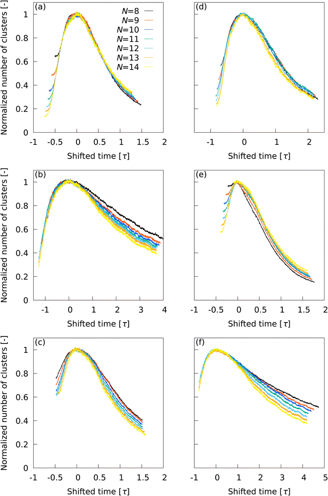 |
| | Fig. 7 Master curves for the time evolution of the total number of clusters observed using (a) ![[Q with combining macron]](https://www.rsc.org/images/entities/i_char_0051_0304.gif) L2, (b) L2, (b) ![[Q with combining macron]](https://www.rsc.org/images/entities/i_char_0051_0304.gif) L12, (c) Ā12, (d) {QL2,QL12}, (e) QL2, and (f) QL12. L12, (c) Ā12, (d) {QL2,QL12}, (e) QL2, and (f) QL12. | |
With ![[Q with combining macron]](https://www.rsc.org/images/entities/i_char_0051_0304.gif) L2, a master curve was obtained that showed little deviation due to differences in N, except for the initial behavior of the transition. The initial behavior of the cluster number and subsequent systematic convergence to the master curve indicates that the impact of errors in
L2, a master curve was obtained that showed little deviation due to differences in N, except for the initial behavior of the transition. The initial behavior of the cluster number and subsequent systematic convergence to the master curve indicates that the impact of errors in ![[Q with combining macron]](https://www.rsc.org/images/entities/i_char_0051_0304.gif) L2 on cluster statistics is almost negligible for N ≥ 12, as implied in Fig. 4.
L2 on cluster statistics is almost negligible for N ≥ 12, as implied in Fig. 4.
A discrepancy was observed in ![[Q with combining macron]](https://www.rsc.org/images/entities/i_char_0051_0304.gif) L12 between curves on the long time range due to the N-dependence in the percolation transition. This trend was also observed for Ā12 and QL12, but appeared to be somewhat improved for {QL2,QL12}. The behavior of QL2 was similar to that of
L12 between curves on the long time range due to the N-dependence in the percolation transition. This trend was also observed for Ā12 and QL12, but appeared to be somewhat improved for {QL2,QL12}. The behavior of QL2 was similar to that of ![[Q with combining macron]](https://www.rsc.org/images/entities/i_char_0051_0304.gif) L2, but the discrepancy due to the difference in N was larger than that of
L2, but the discrepancy due to the difference in N was larger than that of ![[Q with combining macron]](https://www.rsc.org/images/entities/i_char_0051_0304.gif) L2. These results demonstrate the superiority of
L2. These results demonstrate the superiority of ![[Q with combining macron]](https://www.rsc.org/images/entities/i_char_0051_0304.gif) L2 in describing the nucleation and subsequent percolation transition.
L2 in describing the nucleation and subsequent percolation transition.
Overall, the outstanding usefulness of ![[Q with combining macron]](https://www.rsc.org/images/entities/i_char_0051_0304.gif) L2 was demonstrated for all events of the initial stage, nucleation, and percolation transition. The optimal N for
L2 was demonstrated for all events of the initial stage, nucleation, and percolation transition. The optimal N for ![[Q with combining macron]](https://www.rsc.org/images/entities/i_char_0051_0304.gif) L2 is N = 12, because N ≥ 12 is desirable for the initial stage and nucleation, and an unnecessarily large N reduces the cluster resolution.
L2 is N = 12, because N ≥ 12 is desirable for the initial stage and nucleation, and an unnecessarily large N reduces the cluster resolution.
4 Conclusions
In this work, LOPs were selected under an appropriate and efficient screening strategy using MALIO, which enables fast LOP computation and machine learning to evaluate the CTR. MALIO demonstrated superior performance to ML-LSA in LOP computational speed. MALIO achieved a speedup of approximately 17 times even for LOPs with low computational cost, and up to 40 times or more for LOPs with high computational cost. Using the selected LOPs as candidates, the nucleation and subsequent percolation transition were observed to investigate the effect of LOP species and selection of neighboring particles on the cluster statistics. We found the LOP (i.e., ![[Q with combining macron]](https://www.rsc.org/images/entities/i_char_0051_0304.gif) L2) and appropriate number of neighboring particles (N = 12) that accurately describe all events before, during, and after nucleation. The LOP was chosen from among more than 2 million possibilities. The master curve of the time variation of the total number of clusters for each LOP indicates that the LOP is universal in the way it captures the local molecular structures, regardless of the difference in number of neighboring particles. This nature is expected to be confirmed when an LOP is applied to various phase transitions, not only the nematic–smectic transition in this work. Furthermore, the behavior of the percolation transition exhibited by
L2) and appropriate number of neighboring particles (N = 12) that accurately describe all events before, during, and after nucleation. The LOP was chosen from among more than 2 million possibilities. The master curve of the time variation of the total number of clusters for each LOP indicates that the LOP is universal in the way it captures the local molecular structures, regardless of the difference in number of neighboring particles. This nature is expected to be confirmed when an LOP is applied to various phase transitions, not only the nematic–smectic transition in this work. Furthermore, the behavior of the percolation transition exhibited by ![[Q with combining macron]](https://www.rsc.org/images/entities/i_char_0051_0304.gif) L2 clearly indicates that
L2 clearly indicates that ![[Q with combining macron]](https://www.rsc.org/images/entities/i_char_0051_0304.gif) L2 is not only an accurate LOP but also a global order parameter in the percolation transition, and is independent of the number of neighboring particles. This nature of
L2 is not only an accurate LOP but also a global order parameter in the percolation transition, and is independent of the number of neighboring particles. This nature of ![[Q with combining macron]](https://www.rsc.org/images/entities/i_char_0051_0304.gif) L2 is expected to be confirmed when exploring the applicability of LOPs to various phase transition phenomena. Interestingly, this nature of
L2 is expected to be confirmed when exploring the applicability of LOPs to various phase transition phenomena. Interestingly, this nature of ![[Q with combining macron]](https://www.rsc.org/images/entities/i_char_0051_0304.gif) L2 is already implied by MALIO’s screening results.
L2 is already implied by MALIO’s screening results. ![[Q with combining macron]](https://www.rsc.org/images/entities/i_char_0051_0304.gif) L2 is the LOP with the highest CTR at 8 ≤ N ≤ 14, which indicates the accuracy and robustness of
L2 is the LOP with the highest CTR at 8 ≤ N ≤ 14, which indicates the accuracy and robustness of ![[Q with combining macron]](https://www.rsc.org/images/entities/i_char_0051_0304.gif) L2 to a wide range of N. This “signal from machine learning” was substantiated in the actual cluster statistics from nucleation to percolation. This shows that it may be possible to find the optimal LOP directly from the screening strategy used in this work. Of course, this possibility needs to be demonstrated by applying LOPs to a variety of phase transition phenomena, including confined and multicomponent systems, and is a topic for future research. In addition, although MALIO's protocols for neighboring particle selection can in principle be modified to suit the crystal and simulation box geometry, it may be necessary to use only certain protocols for some problems.
L2 to a wide range of N. This “signal from machine learning” was substantiated in the actual cluster statistics from nucleation to percolation. This shows that it may be possible to find the optimal LOP directly from the screening strategy used in this work. Of course, this possibility needs to be demonstrated by applying LOPs to a variety of phase transition phenomena, including confined and multicomponent systems, and is a topic for future research. In addition, although MALIO's protocols for neighboring particle selection can in principle be modified to suit the crystal and simulation box geometry, it may be necessary to use only certain protocols for some problems.
Overall, these results show that machine learning can powerfully screen a huge number of LOP species and suggest only a few promising candidates. We also established a reliable guideline for selecting the number of neighboring particles for LOPs, which has often been a controversial issue. In the future, selecting appropriate LOPs for various phase transitions will lead to deeper understanding of their phenomena and exploration of their potential applications.76
Code availability
MALIO and other codes for analysis are available from the corresponding author upon reasonable request, based on the publication protocol of the developed codes as permitted by a project, JPNP18016, commissioned by the New Energy and Industrial Technology Development Organization (NEDO).
Conflicts of interest
The author declares no conflict of interest.
Acknowledgements
The author thanks Dr Ryuji Sakamaki and Dr Osamu Hino of X-Ability Co., Ltd. for their comprehensive support in developing MALIO. This article is based on results obtained from JPNP18016 commissioned by NEDO, and JST, PRESTO Grant Number JPMJPR22O6, Japan.
Notes and references
-
P. M. Chaikin, T. C. Lubensky and T. A. Witten, Principles of condensed matter physics, Cambridge university press, Cambridge, 1995, vol. 10 Search PubMed.
- T. E. Strzelecka, M. W. Davidson and R. L. Rill, Nature, 1988, 331, 457–460 CrossRef CAS PubMed.
- J. SantaLucia, Proc. Natl. Acad. Sci. U. S. A., 1998, 95, 1460–1465 CrossRef CAS PubMed.
- A. A. Hyman and K. Simons, Science, 2012, 337, 1047–1049 CrossRef CAS PubMed.
- A. A. Hyman, C. A. Weber and F. Jülicher, Annu. Rev. Cell Dev. Biol., 2014, 30, 39–58 CrossRef CAS PubMed.
- S. L. Ilca, X. Sun, K. El Omari, A. Kotecha, F. de Haas, F. DiMaio, J. M. Grimes, D. I. Stuart, M. M. Poranen and J. T. Huiskonen, Nature, 2019, 570, 252–256 CrossRef CAS PubMed.
- T. B. Saw, W. Xi, B. Ladoux and C. T. Lim, Adv. Mater., 2018, 30, 1802579 CrossRef PubMed.
- J. Zhao, U. Gulan, T. Horie, N. Ohmura, J. Han, C. Yang, J. Kong, S. Wang and B. B. Xu, Small, 2019, 15, 1900019 CrossRef PubMed.
- J. S. Langer, Rev. Mod. Phys., 1980, 52, 1 CrossRef CAS.
-
A. Pimpinelli and J. Villain, Physics of Crystal Growth Authors, Cambridge University Press, 1998 DOI:10.1017/CBO9780511622526I.
-
D. Kashchiev, Nucleation, Elsevier, 2000 Search PubMed.
-
E. D. Sloan Jr and C. A. Koh, Clathrate hydrates of natural gases, CRC press, 2007 Search PubMed.
- D. Erdemir, A. Y. Lee and A. S. Myerson, Acc. Chem. Res., 2009, 42, 621–629 CrossRef CAS PubMed.
- P. G. Vekilov, Cryst. Growth Des., 2010, 10, 5007–5019 CrossRef CAS PubMed.
- P. G. Vekilov, Nanoscale, 2010, 2, 2346–2357 RSC.
- W. Qi, Y. Peng, Y. Han, R. K. Bowles and M. Dijkstra, Phys. Rev. Lett., 2015, 115, 185701 CrossRef PubMed.
- M. Salvalaglio, C. Perego, F. Giberti, M. Mazzotti and M. Parrinello, Proc. Natl. Acad. Sci. U. S. A., 2015, 112, E6–E14 CrossRef CAS PubMed.
- G. C. Sosso, J. Chen, S. J. Cox, M. Fitzner, P. Pedevilla, A. Zen and A. Michaelides, Chem. Rev., 2016, 116, 7078–7116 CrossRef CAS PubMed.
- J. F. Lutsko, Sci. Adv., 2019, 5, eaav7399 CrossRef CAS PubMed.
- D. Kashchiev, J. Cryst. Growth, 2020, 530, 125300 CrossRef CAS.
-
J. De Yoreo, Crystallization via Nonclassical Pathways: Nucleation, Assembly, Observation & Application, ACS Publications, vol. 1, 2020, pp. 1–17 Search PubMed.
- S. Auer and D. Frenkel, Nature, 2001, 409, 1020–1023 CrossRef CAS PubMed.
- C. Desgranges and J. Delhommelle, Phys. Rev. Lett., 2007, 98, 235502 CrossRef PubMed.
- M. R. Walsh, C. A. Koh, E. D. Sloan, A. K. Sum and D. T. Wu, Science, 2009, 326, 1095–1098 CrossRef CAS PubMed.
- R. Demichelis, P. Raiteri, J. D. Gale, D. Quigley and D. Gebauer, Nat. Commun., 2011, 2, 590 CrossRef PubMed.
- E. Sanz, C. Vega, J. Espinosa, R. Caballero-Bernal, J. Abascal and C. Valeriani, J. Am. Chem. Soc., 2013, 135, 15008–15017 CrossRef CAS PubMed.
- P. J. Smeets, A. R. Finney, W. J. Habraken, F. Nudelman, H. Friedrich, J. Laven, J. J. De Yoreo, P. M. Rodger and N. A. Sommerdijk, Proc. Natl. Acad. Sci. U. S. A., 2017, 114, E7882–E7890 CrossRef CAS PubMed.
- K. Henzler, E. O. Fetisov, M. Galib, M. D. Baer, B. A. Legg, C. Borca, J. M. Xto, S. Pin, J. L. Fulton and G. K. Schenter,
et al.
, Sci. Adv., 2018, 4, eaao6283 CrossRef PubMed.
- H. Niu, P. M. Piaggi, M. Invernizzi and M. Parrinello, Proc. Natl. Acad. Sci. U. S. A., 2018, 115, 5348–5352 CrossRef CAS PubMed.
- M. Fitzner, G. C. Sosso, S. J. Cox and A. Michaelides, Proc. Natl. Acad. Sci. U. S. A., 2019, 116, 2009–2014 CrossRef CAS PubMed.
- L. Li, J. Zhong, Y. Yan, J. Zhang, J. Xu, J. S. Francisco and X. C. Zeng, Proc. Natl. Acad. Sci. U. S. A., 2020, 117, 24701–24708 CrossRef CAS PubMed.
- K. Z. Takahashi, T. Aoyagi and J.-I. Fukuda, Nat. Commun., 2021, 12, 5278 CrossRef CAS PubMed.
- K. Yasuoka and M. Matsumoto, J. Chem. Phys., 1998, 109, 8451–8462 CrossRef CAS.
- Y. Shibuta, K. Oguchi, T. Takaki and M. Ohno, Sci. Rep., 2015, 5, 1–9 Search PubMed.
- A. Reinhardt, J. P. Doye, E. G. Noya and C. Vega, J. Chem. Phys., 2012, 137, 194504 CrossRef PubMed.
- P. J. Steinhardt, D. R. Nelson and M. Ronchetti, Phys. Rev. B: Condens. Matter Mater. Phys., 1983, 28, 784 CrossRef CAS.
- C. L. Kelchner, S. Plimpton and J. Hamilton, Phys. Rev. B: Condens. Matter Mater. Phys., 1998, 58, 11085 CrossRef CAS.
- G. Ackland and A. Jones, Phys. Rev. B: Condens. Matter Mater. Phys., 2006, 73, 054104 CrossRef.
- W. Lechner and C. Dellago, J. Chem. Phys., 2008, 129, 114707 CrossRef PubMed.
- A. Stukowski, Modell. Simul. Mater. Sci. Eng., 2012, 20, 045021 CrossRef.
- A. Radhi and K. Behdinan, Comput. Mater. Sci., 2017, 126, 182–190 CrossRef CAS.
- H. Doi, K. Z. Takahashi and T. Aoyagi, J. Chem. Phys., 2020, 152, 214501 CrossRef CAS PubMed.
- A. P. Bartók, R. Kondor and G. Csányi, Phys. Rev. B: Condens. Matter Mater. Phys., 2013, 87, 184115 CrossRef.
-
A. Seko, A. Togo and I. Tanaka, Nanoinformatics, Springer, Singapore, 2018, pp. 3–23 Search PubMed.
- H. Doi, K. Z. Takahashi, K. Tagashira, J.-I. Fukuda and T. Aoyagi, Sci. Rep., 2019, 9, 16370 CrossRef PubMed.
- H. Doi, K. Z. Takahashi and T. Aoyagi, J. Chem. Phys., 2021, 154, 164505 CrossRef CAS PubMed.
- H. Doi, K. Z. Takahashi and T. Aoyagi, J. Comput. Chem., 2021, 42, 1720–1727 CrossRef CAS PubMed.
- H. Doi, K. Z. Takahashi and T. Aoyagi, J. Phys. Chem. A, 2021, 125, 9518–9526 CrossRef CAS PubMed.
- M. Fitzner, P. Pedevilla and A. Michaelides, Nat. Commun., 2020, 11, 1–9 CrossRef PubMed.
- Z. Wang, F. Wang, Y. Peng and Y. Han, Nat. Commun., 2015, 6, 6942 CrossRef PubMed.
- W. Mickel, S. C. Kapfer, G. E. Schröder-Turk and K. Mecke, J. Chem. Phys., 2013, 138, 044501 CrossRef PubMed.
- S. Behnel, R. Bradshaw, C. Citro, L. Dalcin, D. S. Seljebotn and K. Smith, Comput. Sci. Eng., 2011, 13, 31–39 Search PubMed.
- G. Albertini, M. Corinaldesi, S. Mazkedian, S. Melone, M. Ponzi-Bossi and F. Rustichelli, Solid State Commun., 1977, 24, 433–437 CrossRef CAS.
- O. Francescangeli, F. Vita and E. T. Samulski, Soft Matter, 2014, 10, 7685–7691 RSC.
- T. Nozawa, P. E. Brumby, S. Ayuba and K. Yasuoka, J. Chem. Phys., 2019, 150, 054903 CrossRef PubMed.
- I. Chuang, N. Turok and B. Yurke, Phys. Rev. Lett., 1991, 66, 2472 CrossRef CAS PubMed.
- I. Chuang, R. Durrer, N. Turok and B. Yurke, Science, 1991, 251, 1336–1342 CrossRef CAS PubMed.
- S. Plimpton, J. Comput. Phys., 1995, 117, 1–19 CrossRef CAS.
- R. Berardi, A. P. J. Emerson and C. Zannoni, J. Chem. Soc., Faraday Trans., 1993, 89, 4069–4078 RSC.
- R. Berardi, J. S. Lintuvuori, M. R. Wilson and C. Zannoni, J. Chem. Phys., 2011, 135, 134119 CrossRef PubMed.
- R. Berardi, C. Zannoni, J. S. Lintuvuori and M. R. Wilson, J. Chem. Phys., 2009, 131, 174107 CrossRef PubMed.
- K. Mochizuki, M. Matsumoto and I. Ohmine, Nature, 2013, 498, 350–354 CrossRef CAS PubMed.
- J. D. Honeycutt and H. C. Andersen, J. Phys. Chem., 1987, 91, 4950–4963 CrossRef CAS.
- E. Maras, O. Trushin, A. Stukowski, T. Ala-Nissila and H. Jonsson, Comput. Phys. Commun., 2016, 205, 13–21 CrossRef CAS.
- P.-L. Chau and A. Hardwick, Mol. Phys., 1998, 93, 511–518 CrossRef CAS.
- E. Duboué-Dijon and D. Laage, J. Phys. Chem. B, 2015, 119, 8406–8418 CrossRef PubMed.
- E. B. Moore, E. De La Llave, K. Welke, D. A. Scherlis and V. Molinero, Phys. Chem. Chem. Phys., 2010, 12, 4124–4134 RSC.
- L. Onsager, Ann. N. Y. Acad. Sci., 1949, 51, 627–659 CrossRef CAS.
- W. L. McMillan, Phys. Rev. A: At., Mol., Opt. Phys., 1971, 4, 1238 CrossRef.
-
B. Boots, K. Sugihara, S. N. Chiu and A. Okabe, Spatial tessellations: concepts and applications of Voronoi diagrams, John Wiley & Sons, 2009 Search PubMed.
- W. F. Reinhart and A. Z. Panagiotopoulos, Soft Matter, 2018, 14, 6083–6089 RSC.
- F. Pedregosa, G. Varoquaux, A. Gramfort, V. Michel, B. Thirion, O. Grisel, M. Blondel, P. Prettenhofer, R. Weiss, V. Dubourg, J. Vanderplas, A. Passos, D. Cournapeau, M. Brucher, M. Perrot and E. Duchesnay, J. Mach. Learn. Res., 2011, 12, 2825–2830 Search PubMed.
- A. Jain and D. Zongker, IEEE transactions on pattern analysis and machine intelligence, 1997, 19, 153–158 CrossRef.
- M. A. Bates and G. R. Luckhurst, J. Chem. Phys., 2003, 118, 6605–6614 CrossRef CAS.
- G. Skačej and C. Zannoni, Proc. Natl. Acad. Sci. U. S. A., 2012, 109, 10193–10198 CrossRef PubMed.
- K. E. Blow, D. Quigley and G. C. Sosso, J. Chem. Phys., 2021, 155, 040901 CrossRef CAS PubMed.
|
| This journal is © the Owner Societies 2023 |
Click here to see how this site uses Cookies. View our privacy policy here.  Open Access Article
 *
*


 and
and  denote the contributions corresponding to the well depth and configuration anisotropies, and μ and ν are multipliers for determining these two contributions to the pair potential. The factor
  is characterized by introducing a parameter
  , where
  and
and  denote energy contributions from the end-to-end and side-by-side ellipsoid configurations, respectively. The factor
  is characterized by κ. Therefore, the detailed shape of UGB is determined from the values of the four parameters κ, κ′, μ, and ν. We set κ = 3, κ′ = 5, μ = 1, and ν = 3. Note that the above parameter set has been traditionally used because the physical properties of nematic and smectic B liquid crystal phases are well displayed.59,60 For the characteristic length, energy, and mass of the SCGB systems, σ = σs, ε = kBT, and m are each set to 1; here, m is the mass of one SCGB particle. The terms a and b were set to −70εσ−1 and −100σ−1, respectively, on the basis of previous reports.60,61 Using the above parameter settings, the nematic–smectic transition is guaranteed to be observed for SCGB systems by quenching from temperature T = 2.4 to 1.8 at a density of 0.3σ−3.60 Therefore, an ensemble was used having a constant number of particles at a density of 0.3σ−3 contained within a cubic box of constant volume and temperature with full periodic boundary conditions imposed. The initial configurations for the nematic–smectic phase transition trajectory were prepared carefully by being cooled gradually from the isotropic phase at T = 6.0 to the nematic phase at T = 2.4. The configurations were then quenched to T = 1.8 below the nematic–smectic transition temperature TN–Sm = 2.25. To observe the fast nucleation during the weak first-order phase transition, a velocity Verlet integrator with a fine timestep of 2.0 × 10⁻⁵τ was used for SCGB, where τ = (mσ/ε)1/2 is a time unit. The temperature was controlled using a Nosé–Hoover chain thermostat.62 The SCGB potential was truncated at 8.0σ to precisely compute the intermolecular interactions during the phase transition.


![[B with combining macron]](https://www.rsc.org/images/entities/i_char_0042_0304.gif) is defined as
is defined as

 is an array including the identifiers of neighbor beads of half of Nb(i) in order of nearest neighbor from particle i, N′ denotes the number of elements in array
  and k satisfies the relation k = j + N − N′. The locally averaged neighborhood parameter
 ![[C with combining macron]](https://www.rsc.org/images/entities/i_char_0043_0304.gif) is defined as
is defined as

![[D with combining macron]](https://www.rsc.org/images/entities/i_char_0044_0304.gif) is defined as
is defined as

![[F with combining macron]](https://www.rsc.org/images/entities/i_char_0046_0304.gif) is defined as
is defined as
![[H with combining macron]](https://www.rsc.org/images/entities/i_char_0048_0304.gif) is defined as
is defined as


![[Q with combining macron]](https://www.rsc.org/images/entities/i_char_0051_0304.gif) S and
S and ![[W with combining macron]](https://www.rsc.org/images/entities/i_char_0057_0304.gif) S are defined as
S are defined as


![[Q with combining macron]](https://www.rsc.org/images/entities/i_char_0051_0304.gif) L and
L and ![[W with combining macron]](https://www.rsc.org/images/entities/i_char_0057_0304.gif) L are defined as
L are defined as


![[L with combining macron]](https://www.rsc.org/images/entities/i_char_004c_0304.gif) Q and
Q and ![[L with combining macron]](https://www.rsc.org/images/entities/i_char_004c_0304.gif) W are defined as
W are defined as


![[L with combining macron]](https://www.rsc.org/images/entities/i_char_004c_0304.gif) QM and
QM and ![[L with combining macron]](https://www.rsc.org/images/entities/i_char_004c_0304.gif) WM are defined as
WM are defined as


![[S with combining macron]](https://www.rsc.org/images/entities/i_char_0053_0304.gif) is defined as
is defined as

![[T with combining macron]](https://www.rsc.org/images/entities/i_char_0054_0304.gif) is defined as
is defined as
![[thin space (1/6-em)]](https://www.rsc.org/images/entities/char_2009.gif) 220
220![[thin space (1/6-em)]](https://www.rsc.org/images/entities/char_2009.gif) 777 (=(702C1 + 702C2) × 9 neighboring conditions) different combinations of LOPs were considered.
777 (=(702C1 + 702C2) × 9 neighboring conditions) different combinations of LOPs were considered.![[thin space (1/6-em)]](https://www.rsc.org/images/entities/char_2009.gif) 400 (= 1701 particles × 200 coordinate data × 2 phases) of Lis. The structure name (nematic or smectic) was tagged onto each Li and designated as the objective variable. (iv) The structure descriptors and objective variables were then stored in the descriptor array Ds and the structure name vector n, respectively. (v) Finally, the random forest method implemented in Scikit-learn (version 0.20.3)72 was used to estimate the operator vector w satisfying the relation Dsw = n. The number of trees in the forest was set to 100, and the maximum depth of each tree was set to 10. Default values in Scikit-learn were used for the other settings. The quality of w was also checked by 5-fold cross-validation implemented in Scikit-learn. The combination of two LOPs can be considered by arbitrarily selecting two of the elements of w and setting the others to null. This process was carried out using a sequential forward selection algorithm.73 The classification accuracy of each (set of) LOP(s) was calculated from the correct tagging rate (CTR) as implemented in MALIO. The CTR c is defined as
400 (= 1701 particles × 200 coordinate data × 2 phases) of Lis. The structure name (nematic or smectic) was tagged onto each Li and designated as the objective variable. (iv) The structure descriptors and objective variables were then stored in the descriptor array Ds and the structure name vector n, respectively. (v) Finally, the random forest method implemented in Scikit-learn (version 0.20.3)72 was used to estimate the operator vector w satisfying the relation Dsw = n. The number of trees in the forest was set to 100, and the maximum depth of each tree was set to 10. Default values in Scikit-learn were used for the other settings. The quality of w was also checked by 5-fold cross-validation implemented in Scikit-learn. The combination of two LOPs can be considered by arbitrarily selecting two of the elements of w and setting the others to null. This process was carried out using a sequential forward selection algorithm.73 The classification accuracy of each (set of) LOP(s) was calculated from the correct tagging rate (CTR) as implemented in MALIO. The CTR c is defined as
![[Q with combining macron]](https://www.rsc.org/images/entities/i_char_0051_0304.gif) L2 is the LOP calculated by MALIO's original spherical harmonic function library, and
L2 is the LOP calculated by MALIO's original spherical harmonic function library, and ![[S with combining macron]](https://www.rsc.org/images/entities/i_char_0053_0304.gif) 2 is the LOP with relatively low computational cost. In ML-LSA, the computational time for Ā12 and
2 is the LOP with relatively low computational cost. In ML-LSA, the computational time for Ā12 and ![[Q with combining macron]](https://www.rsc.org/images/entities/i_char_0051_0304.gif) L2 increased with increasing N, while the computational time for
L2 increased with increasing N, while the computational time for ![[S with combining macron]](https://www.rsc.org/images/entities/i_char_0053_0304.gif) 2 hardly increased with increasing N. In MALIO, the computational time was much shorter than in ML-LSA. The computational time for Ā12 increased with increasing N, while the computational time for
2 hardly increased with increasing N. In MALIO, the computational time was much shorter than in ML-LSA. The computational time for Ā12 increased with increasing N, while the computational time for ![[Q with combining macron]](https://www.rsc.org/images/entities/i_char_0051_0304.gif) L2 and
L2 and ![[S with combining macron]](https://www.rsc.org/images/entities/i_char_0053_0304.gif) 2 hardly increased with increasing N. Efficient computation of
2 hardly increased with increasing N. Efficient computation of ![[Q with combining macron]](https://www.rsc.org/images/entities/i_char_0051_0304.gif) L2 by MALIO's original spherical harmonic function calculation library resulted in saturation of
L2 by MALIO's original spherical harmonic function calculation library resulted in saturation of ![[Q with combining macron]](https://www.rsc.org/images/entities/i_char_0051_0304.gif) L2 computational time with respect to N. The ratio of LOP computational time for ML-LSA to that for MALIO reveals a dramatic speedup in LOP computational time with MALIO. A maximum speedup of over 40 times was achieved in Ā12, and a maximum speedup of over 35 times was achieved in
L2 computational time with respect to N. The ratio of LOP computational time for ML-LSA to that for MALIO reveals a dramatic speedup in LOP computational time with MALIO. A maximum speedup of over 40 times was achieved in Ā12, and a maximum speedup of over 35 times was achieved in ![[Q with combining macron]](https://www.rsc.org/images/entities/i_char_0051_0304.gif) L2. Even in
L2. Even in ![[S with combining macron]](https://www.rsc.org/images/entities/i_char_0053_0304.gif) 2, where the computational cost is relatively low, a speedup of over 17 times was achieved.
2, where the computational cost is relatively low, a speedup of over 17 times was achieved.
![[Q with combining macron]](https://www.rsc.org/images/entities/i_char_0051_0304.gif) L series was found to be the best single LOP for all N conditions. In particular,
L series was found to be the best single LOP for all N conditions. In particular, ![[Q with combining macron]](https://www.rsc.org/images/entities/i_char_0051_0304.gif) L2 attained the best CTR for N ≥ 8 and was the most robust to N. The best set of two LOPs was also found to be the combination of the
L2 attained the best CTR for N ≥ 8 and was the most robust to N. The best set of two LOPs was also found to be the combination of the ![[Q with combining macron]](https://www.rsc.org/images/entities/i_char_0051_0304.gif) L series (chosen as the best single LOP) and the QL series for all N conditions. However, the improvement in c due to adding the QL series was small (less than 0.01 for almost all N), and the increase in the number of LOPs was not commensurate with the CTR increase. Recall that in additional analyses such as drawing free energy landscapes, increasing the number of LOPs leads directly to an exponential increase in computational cost due to the curse of dimensionality, and makes it less easy to interpret results. A single LOP should be used in the above cases. The second- and third-best LOPs also fall into this case.
L series (chosen as the best single LOP) and the QL series for all N conditions. However, the improvement in c due to adding the QL series was small (less than 0.01 for almost all N), and the increase in the number of LOPs was not commensurate with the CTR increase. Recall that in additional analyses such as drawing free energy landscapes, increasing the number of LOPs leads directly to an exponential increase in computational cost due to the curse of dimensionality, and makes it less easy to interpret results. A single LOP should be used in the above cases. The second- and third-best LOPs also fall into this case.
![[Q with combining macron]](https://www.rsc.org/images/entities/i_char_0051_0304.gif) L6 (0.978 ± 0.004)
L6 (0.978 ± 0.004)![[Q with combining macron]](https://www.rsc.org/images/entities/i_char_0051_0304.gif) L6 (0.977 ± 0.004)
L6 (0.977 ± 0.004)![[Q with combining macron]](https://www.rsc.org/images/entities/i_char_0051_0304.gif) L2 (0.959 ± 0.008)
L2 (0.959 ± 0.008)![[Q with combining macron]](https://www.rsc.org/images/entities/i_char_0051_0304.gif) L2 (0.976 ± 0.005)
L2 (0.976 ± 0.005)![[Q with combining macron]](https://www.rsc.org/images/entities/i_char_0051_0304.gif) L12 (0.974 ± 0.004)
L12 (0.974 ± 0.004)![[Q with combining macron]](https://www.rsc.org/images/entities/i_char_0051_0304.gif) L6 (0.969 ± 0.004)
L6 (0.969 ± 0.004)![[Q with combining macron]](https://www.rsc.org/images/entities/i_char_0051_0304.gif) L2 (0.985 ± 0.004)
L2 (0.985 ± 0.004)![[Q with combining macron]](https://www.rsc.org/images/entities/i_char_0051_0304.gif) L12 (0.982 ± 0.004)
L12 (0.982 ± 0.004)![[F with combining macron]](https://www.rsc.org/images/entities/i_char_0046_0304.gif) f
3,f3,6.0 (0.973 ± 0.004)
f
3,f3,6.0 (0.973 ± 0.004)![[Q with combining macron]](https://www.rsc.org/images/entities/i_char_0051_0304.gif) L2 (0.991 ± 0.003)
L2 (0.991 ± 0.003)![[Q with combining macron]](https://www.rsc.org/images/entities/i_char_0051_0304.gif) L12 (0.987 ± 0.003)
L12 (0.987 ± 0.003)![[Q with combining macron]](https://www.rsc.org/images/entities/i_char_0051_0304.gif) L2 (0.994 ± 0.002)
L2 (0.994 ± 0.002)![[Q with combining macron]](https://www.rsc.org/images/entities/i_char_0051_0304.gif) L12 (0.990 ± 0.003)
L12 (0.990 ± 0.003)![[Q with combining macron]](https://www.rsc.org/images/entities/i_char_0051_0304.gif) L2 (0.996 ± 0.001)
L2 (0.996 ± 0.001)![[Q with combining macron]](https://www.rsc.org/images/entities/i_char_0051_0304.gif) L12 (0.992 ± 0.002)
L12 (0.992 ± 0.002)![[Q with combining macron]](https://www.rsc.org/images/entities/i_char_0051_0304.gif) L2 (0.997 ± 0.001)
L2 (0.997 ± 0.001)![[Q with combining macron]](https://www.rsc.org/images/entities/i_char_0051_0304.gif) L12 (0.994 ± 0.002)
L12 (0.994 ± 0.002)![[B with combining macron]](https://www.rsc.org/images/entities/i_char_0042_0304.gif) 1,3,π/6 (0.988 ± 0.004)
1,3,π/6 (0.988 ± 0.004)![[Q with combining macron]](https://www.rsc.org/images/entities/i_char_0051_0304.gif) L2 (0.998 ± 0.001)
L2 (0.998 ± 0.001)![[Q with combining macron]](https://www.rsc.org/images/entities/i_char_0051_0304.gif) L12 (0.995 ± 0.002)
L12 (0.995 ± 0.002)![[B with combining macron]](https://www.rsc.org/images/entities/i_char_0042_0304.gif) 1,3,π/6 (0.991 ± 0.004)
1,3,π/6 (0.991 ± 0.004)![[Q with combining macron]](https://www.rsc.org/images/entities/i_char_0051_0304.gif) L6,QL6} (0.988 ± 0.003)
L6,QL6} (0.988 ± 0.003)![[Q with combining macron]](https://www.rsc.org/images/entities/i_char_0051_0304.gif) L5} (0.968 ± 0.006)
L5} (0.968 ± 0.006)![[Q with combining macron]](https://www.rsc.org/images/entities/i_char_0051_0304.gif) L5} (0.967 ± 0.005)
L5} (0.967 ± 0.005)![[Q with combining macron]](https://www.rsc.org/images/entities/i_char_0051_0304.gif) L6,QL6} (0.986 ± 0.003)
L6,QL6} (0.986 ± 0.003)![[Q with combining macron]](https://www.rsc.org/images/entities/i_char_0051_0304.gif) L2,
L2,![[Q with combining macron]](https://www.rsc.org/images/entities/i_char_0051_0304.gif) L12} (0.981 ± 0.004)
L12} (0.981 ± 0.004)![[Q with combining macron]](https://www.rsc.org/images/entities/i_char_0051_0304.gif) L12} (0.976 ± 0.005)
L12} (0.976 ± 0.005)![[Q with combining macron]](https://www.rsc.org/images/entities/i_char_0051_0304.gif) L2,QL2} (0.989 ± 0.003)
L2,QL2} (0.989 ± 0.003)![[Q with combining macron]](https://www.rsc.org/images/entities/i_char_0051_0304.gif) L12,
L12,![[Q with combining macron]](https://www.rsc.org/images/entities/i_char_0051_0304.gif) L4} (0.984 ± 0.004)
L4} (0.984 ± 0.004)![[Q with combining macron]](https://www.rsc.org/images/entities/i_char_0051_0304.gif) L6,
L6,![[B with combining macron]](https://www.rsc.org/images/entities/i_char_0042_0304.gif) 1,1,π/4} (0.981 ± 0.004)
1,1,π/4} (0.981 ± 0.004)![[Q with combining macron]](https://www.rsc.org/images/entities/i_char_0051_0304.gif) L2,QL2} (0.994 ± 0.002)
L2,QL2} (0.994 ± 0.002)![[Q with combining macron]](https://www.rsc.org/images/entities/i_char_0051_0304.gif) L12,
L12,![[Q with combining macron]](https://www.rsc.org/images/entities/i_char_0051_0304.gif) L4} (0.990 ± 0.003)
L4} (0.990 ± 0.003)![[F with combining macron]](https://www.rsc.org/images/entities/i_char_0046_0304.gif) f3,f2,6.0,
f3,f2,6.0,![[S with combining macron]](https://www.rsc.org/images/entities/i_char_0053_0304.gif) 2} (0.983 ± 0.003)
2} (0.983 ± 0.003)![[Q with combining macron]](https://www.rsc.org/images/entities/i_char_0051_0304.gif) L2,QL2} (0.997 ± 0.001)
L2,QL2} (0.997 ± 0.001)![[Q with combining macron]](https://www.rsc.org/images/entities/i_char_0051_0304.gif) L12,QL12} (0.993 ± 0.002)
L12,QL12} (0.993 ± 0.002)![[W with combining macron]](https://www.rsc.org/images/entities/i_char_0057_0304.gif) L2} (0.985 ± 0.004)
L2} (0.985 ± 0.004)![[Q with combining macron]](https://www.rsc.org/images/entities/i_char_0051_0304.gif) L2,QL2} (0.998 ± 0.001)
L2,QL2} (0.998 ± 0.001)![[Q with combining macron]](https://www.rsc.org/images/entities/i_char_0051_0304.gif) L12,QL12} (0.995 ± 0.002)
L12,QL12} (0.995 ± 0.002)![[W with combining macron]](https://www.rsc.org/images/entities/i_char_0057_0304.gif) L2} (0.988 ± 0.004)
L2} (0.988 ± 0.004)![[Q with combining macron]](https://www.rsc.org/images/entities/i_char_0051_0304.gif) L2,QL2} (0.999 ± 0.001)
L2,QL2} (0.999 ± 0.001)![[Q with combining macron]](https://www.rsc.org/images/entities/i_char_0051_0304.gif) L12,QL12} (0.997 ± 0.001)
L12,QL12} (0.997 ± 0.001)![[W with combining macron]](https://www.rsc.org/images/entities/i_char_0057_0304.gif) L2} (0.990 ± 0.004)
L2} (0.990 ± 0.004)![[Q with combining macron]](https://www.rsc.org/images/entities/i_char_0051_0304.gif) L2,QL2} (1.000 ± 0.000)
L2,QL2} (1.000 ± 0.000)![[Q with combining macron]](https://www.rsc.org/images/entities/i_char_0051_0304.gif) L12,QL12} (0.998 ± 0.001)
L12,QL12} (0.998 ± 0.001)![[B with combining macron]](https://www.rsc.org/images/entities/i_char_0042_0304.gif) 1,3,π/6,
1,3,π/6,![[W with combining macron]](https://www.rsc.org/images/entities/i_char_0057_0304.gif) L2} (0.994 ± 0.003)
L2} (0.994 ± 0.003)![[Q with combining macron]](https://www.rsc.org/images/entities/i_char_0051_0304.gif) L2,QL2} (1.000 ± 0.000)
L2,QL2} (1.000 ± 0.000)![[Q with combining macron]](https://www.rsc.org/images/entities/i_char_0051_0304.gif) L12,QL12} (0.998 ± 0.001)
L12,QL12} (0.998 ± 0.001)![[B with combining macron]](https://www.rsc.org/images/entities/i_char_0042_0304.gif) 1,3,π/6,
1,3,π/6,![[W with combining macron]](https://www.rsc.org/images/entities/i_char_0057_0304.gif) L2} (0.996 ± 0.002)
L2} (0.996 ± 0.002)![[Q with combining macron]](https://www.rsc.org/images/entities/i_char_0051_0304.gif) L6,
L6, ![[Q with combining macron]](https://www.rsc.org/images/entities/i_char_0051_0304.gif) L2,
L2, ![[Q with combining macron]](https://www.rsc.org/images/entities/i_char_0051_0304.gif) L12, Ā12, {QL2,QL12}, QL2, and QL12.
L12, Ā12, {QL2,QL12}, QL2, and QL12.![[Q with combining macron]](https://www.rsc.org/images/entities/i_char_0051_0304.gif) L6 is the best LOP. Therefore, we first observed the cluster statistics when
L6 is the best LOP. Therefore, we first observed the cluster statistics when ![[Q with combining macron]](https://www.rsc.org/images/entities/i_char_0051_0304.gif) L6 was used. Fig. 3 shows (a) the time evolution of the number of smectic molecules in the system and in the maximum cluster, and (b) the ratio of the number of molecules in the largest cluster to the number of smectic molecules in the system. The time evolution of Onsager's global order parameter was also plotted in Fig. 3(b). With the CTR of
L6 was used. Fig. 3 shows (a) the time evolution of the number of smectic molecules in the system and in the maximum cluster, and (b) the ratio of the number of molecules in the largest cluster to the number of smectic molecules in the system. The time evolution of Onsager's global order parameter was also plotted in Fig. 3(b). With the CTR of ![[Q with combining macron]](https://www.rsc.org/images/entities/i_char_0051_0304.gif) L6 for N = 6 and 7 (c ∼ 0.98), a number of smectic molecules were detected even in the initial structure, which should be completely in the nematic phase. This depends completely on the CTRs in Table 2, implying that extremely high CTRs are required to observe cluster statistics in nucleation. At t = 5.0 τ, the total number of smectic molecules reached about 400
L6 for N = 6 and 7 (c ∼ 0.98), a number of smectic molecules were detected even in the initial structure, which should be completely in the nematic phase. This depends completely on the CTRs in Table 2, implying that extremely high CTRs are required to observe cluster statistics in nucleation. At t = 5.0 τ, the total number of smectic molecules reached about 400![[thin space (1/6-em)]](https://www.rsc.org/images/entities/char_2009.gif) 000. However, it is clear from Fig. 3(b) that the largest cluster did not grow at all until t = 5.0 τ. The results indicate that the transition does not progress from nucleation to percolation, even though approximately 40% of the molecules are determined to be smectic molecules. The same trend was observed for other LOP species when N = 6 and 7 were used (data not shown). This unnatural behavior indicates that N is too small and is insufficient to capture the smectic layer. Therefore, in the following analysis, the conditions N = 8–14 were used and
000. However, it is clear from Fig. 3(b) that the largest cluster did not grow at all until t = 5.0 τ. The results indicate that the transition does not progress from nucleation to percolation, even though approximately 40% of the molecules are determined to be smectic molecules. The same trend was observed for other LOP species when N = 6 and 7 were used (data not shown). This unnatural behavior indicates that N is too small and is insufficient to capture the smectic layer. Therefore, in the following analysis, the conditions N = 8–14 were used and ![[Q with combining macron]](https://www.rsc.org/images/entities/i_char_0051_0304.gif) L6 was excluded. Note that Onsager's global order parameter was also insensitive to increases in the number of smectic molecules.
L6 was excluded. Note that Onsager's global order parameter was also insensitive to increases in the number of smectic molecules.
![[Q with combining macron]](https://www.rsc.org/images/entities/i_char_0051_0304.gif) L2, (b)
L2, (b) ![[Q with combining macron]](https://www.rsc.org/images/entities/i_char_0051_0304.gif) L12, (c) Ā12, (d) {QL2,QL12}, (e) QL2, and (f) QL12. The number of smectic molecules was divided by the total number of molecules. The initially observed smectic molecules originate from the error in classification using LOPs. With
L12, (c) Ā12, (d) {QL2,QL12}, (e) QL2, and (f) QL12. The number of smectic molecules was divided by the total number of molecules. The initially observed smectic molecules originate from the error in classification using LOPs. With ![[Q with combining macron]](https://www.rsc.org/images/entities/i_char_0051_0304.gif) L2, the number of initial smectic molecules could be suppressed to less than 0.5% for N ≥ 12. That the number of molecules hardly increased with time up to t > 0.1τ independently of N is consistent with the fact that cluster formation is less likely to proceed in the initial nucleation stage.
L2, the number of initial smectic molecules could be suppressed to less than 0.5% for N ≥ 12. That the number of molecules hardly increased with time up to t > 0.1τ independently of N is consistent with the fact that cluster formation is less likely to proceed in the initial nucleation stage.
![[Q with combining macron]](https://www.rsc.org/images/entities/i_char_0051_0304.gif) L12, the number of initial smectic molecules could be suppressed to less than 1% for N ≥ 13, but the observed number of smectic molecules increased immediately afterwards. With Ā12, the number of initial smectic molecules could not be suppressed to less than 1% for any of the N conditions, nor could the increase in the number of smectic molecules immediately afterwards be suppressed. With {QL2,QL12}, the number of initial smectic molecules could be suppressed to less than 1% for N ≥ 12, but the number of smectic molecules increased immediately afterwards. With QL2, the number of initial smectic molecules could not be suppressed to less than 1% for any of the N conditions, but its increase with time at t > 0.1τ was similar to that for
L12, the number of initial smectic molecules could be suppressed to less than 1% for N ≥ 13, but the observed number of smectic molecules increased immediately afterwards. With Ā12, the number of initial smectic molecules could not be suppressed to less than 1% for any of the N conditions, nor could the increase in the number of smectic molecules immediately afterwards be suppressed. With {QL2,QL12}, the number of initial smectic molecules could be suppressed to less than 1% for N ≥ 12, but the number of smectic molecules increased immediately afterwards. With QL2, the number of initial smectic molecules could not be suppressed to less than 1% for any of the N conditions, but its increase with time at t > 0.1τ was similar to that for ![[Q with combining macron]](https://www.rsc.org/images/entities/i_char_0051_0304.gif) L2. With QL12, the number of initial smectic molecules could not be suppressed to less than 1% for any of the N conditions, nor could the increase in number of smectic molecules immediately afterwards be suppressed. The results indicate the superiority of
L2. With QL12, the number of initial smectic molecules could not be suppressed to less than 1% for any of the N conditions, nor could the increase in number of smectic molecules immediately afterwards be suppressed. The results indicate the superiority of ![[Q with combining macron]](https://www.rsc.org/images/entities/i_char_0051_0304.gif) L2.
L2.![[Q with combining macron]](https://www.rsc.org/images/entities/i_char_0051_0304.gif) L2, (b)
L2, (b) ![[Q with combining macron]](https://www.rsc.org/images/entities/i_char_0051_0304.gif) L12, (c) Ā12, (d) {QL2,QL12}, (e) QL2, and (f) QL12. The Onsager's order parameter and the all-particle mean of
L12, (c) Ā12, (d) {QL2,QL12}, (e) QL2, and (f) QL12. The Onsager's order parameter and the all-particle mean of ![[Q with combining macron]](https://www.rsc.org/images/entities/i_char_0051_0304.gif) L2, 〈
L2, 〈![[Q with combining macron]](https://www.rsc.org/images/entities/i_char_0051_0304.gif) L2〉, were also plotted to show the time evolution of global order parameters. A rapid increase in the ratio signifies the onset of percolation, and the onset of convergence to 1 signifies completion of percolation. With
L2〉, were also plotted to show the time evolution of global order parameters. A rapid increase in the ratio signifies the onset of percolation, and the onset of convergence to 1 signifies completion of percolation. With ![[Q with combining macron]](https://www.rsc.org/images/entities/i_char_0051_0304.gif) L2, the curves overlapped for all N conditions, indicating that the percolation onset and completion times were independent of N. The completion time (t ∼ 1.5τ) agreed perfectly with the results of numerical analysis corresponding to X-ray scattering experiments on liquid crystal molecular systems undergoing phase transition. Fig. 6 shows the time evolution of X-ray scattering intensity calculated for the liquid crystal molecular systems during the phase transition. The time evolution of scattering intensity was calculated using the following procedure: (i) the scattering pattern at each time was calculated on the basis of previous studies.74,75 (ii) Because the intensity difference between the two phases is larger near the second harmonic according to previous studies,32,74,75 the intensity at each time was integrated over a rectangular region cut in the ranges −3.5σ−1 ≤ qa ≤ 3.5σ−1 and 3.5σ−1 ≤ qb ≤ 6.0σ−1, where qa and qb are the wavenumbers of the components perpendicular and parallel to the liquid crystal orientation direction, respectively. Because the X-ray analysis is performed completely independently from the various analyses using LOPs, it can be used as one indicator to evaluate LOP performance. The X-ray intensity increased almost linearly for 0 ≤ t ≤ 1.475τ. However, for t > 1.475τ, the increasing trend became gradual and intermittent. The results show that the smectic local structures complete percolation at t = 1.475τ, implying the number of smectic molecules in the largest cluster becomes almost equal to the number of total smectic molecules in the system.
L2, the curves overlapped for all N conditions, indicating that the percolation onset and completion times were independent of N. The completion time (t ∼ 1.5τ) agreed perfectly with the results of numerical analysis corresponding to X-ray scattering experiments on liquid crystal molecular systems undergoing phase transition. Fig. 6 shows the time evolution of X-ray scattering intensity calculated for the liquid crystal molecular systems during the phase transition. The time evolution of scattering intensity was calculated using the following procedure: (i) the scattering pattern at each time was calculated on the basis of previous studies.74,75 (ii) Because the intensity difference between the two phases is larger near the second harmonic according to previous studies,32,74,75 the intensity at each time was integrated over a rectangular region cut in the ranges −3.5σ−1 ≤ qa ≤ 3.5σ−1 and 3.5σ−1 ≤ qb ≤ 6.0σ−1, where qa and qb are the wavenumbers of the components perpendicular and parallel to the liquid crystal orientation direction, respectively. Because the X-ray analysis is performed completely independently from the various analyses using LOPs, it can be used as one indicator to evaluate LOP performance. The X-ray intensity increased almost linearly for 0 ≤ t ≤ 1.475τ. However, for t > 1.475τ, the increasing trend became gradual and intermittent. The results show that the smectic local structures complete percolation at t = 1.475τ, implying the number of smectic molecules in the largest cluster becomes almost equal to the number of total smectic molecules in the system.
![[Q with combining macron]](https://www.rsc.org/images/entities/i_char_0051_0304.gif) L12, the curves for the different N conditions did not overlap each other. The completion time of percolation deviated from the X-ray intensity results for all N conditions, but the two sets of results became closer with increasing N. With Ā12, the curves for different N conditions did not overlap each other. Interestingly, curves relatively close to the
L12, the curves for the different N conditions did not overlap each other. The completion time of percolation deviated from the X-ray intensity results for all N conditions, but the two sets of results became closer with increasing N. With Ā12, the curves for different N conditions did not overlap each other. Interestingly, curves relatively close to the ![[Q with combining macron]](https://www.rsc.org/images/entities/i_char_0051_0304.gif) L2 results were obtained at 10≤ N ≤ 12, where the performance of Ā12 was third-best (see Table 2). The curves for different N conditions did not overlap with each other with {QL2,QL12}, although the results appeared to be slightly improved over the
L2 results were obtained at 10≤ N ≤ 12, where the performance of Ā12 was third-best (see Table 2). The curves for different N conditions did not overlap with each other with {QL2,QL12}, although the results appeared to be slightly improved over the ![[Q with combining macron]](https://www.rsc.org/images/entities/i_char_0051_0304.gif) L12 results. The percolation completion time tended to be closer to the X-ray intensity results as N was increased. A master curve similar to the
L12 results. The percolation completion time tended to be closer to the X-ray intensity results as N was increased. A master curve similar to the ![[Q with combining macron]](https://www.rsc.org/images/entities/i_char_0051_0304.gif) L2 results was obtained with QL2, but the overlap between the curves was not as exact as with
L2 results was obtained with QL2, but the overlap between the curves was not as exact as with ![[Q with combining macron]](https://www.rsc.org/images/entities/i_char_0051_0304.gif) L2. With QL12, the results were inferior to the
L2. With QL12, the results were inferior to the ![[Q with combining macron]](https://www.rsc.org/images/entities/i_char_0051_0304.gif) L12 results.
L12 results.![[Q with combining macron]](https://www.rsc.org/images/entities/i_char_0051_0304.gif) L2 was pronounced in describing percolation transitions. The effectiveness of the LOP local average and the effect of LOP combinations were also evident. The sensitivity of the global order parameters to the percolation transition was extremely low, showing only an almost monotonically increasing trend without any response to the transition time. This fact indicates that it is difficult to detect the details of molecular self-assembly dynamics with global order parameters.
L2 was pronounced in describing percolation transitions. The effectiveness of the LOP local average and the effect of LOP combinations were also evident. The sensitivity of the global order parameters to the percolation transition was extremely low, showing only an almost monotonically increasing trend without any response to the transition time. This fact indicates that it is difficult to detect the details of molecular self-assembly dynamics with global order parameters.![[Q with combining macron]](https://www.rsc.org/images/entities/i_char_0051_0304.gif) L2, (b)
L2, (b) ![[Q with combining macron]](https://www.rsc.org/images/entities/i_char_0051_0304.gif) L12, (c) Ā12, (d) {QL2,QL12}, (e) QL2, and (f) QL12. For the same LOP, when the time at which the number of clusters reaches its maximum is shifted to zero and the number of clusters is normalized using the maximum value, the time evolution of the total number of clusters shows one characteristic curve despite the use of different N values. The results show the nature of each LOP is independent of the number of neighboring particles in the cluster statistics. Although the actual number of clusters varies with N, the time evolution of the cluster number is similar for all N values, demonstrating a strong universality in the way clusters are captured by an LOP.
L12, (c) Ā12, (d) {QL2,QL12}, (e) QL2, and (f) QL12. For the same LOP, when the time at which the number of clusters reaches its maximum is shifted to zero and the number of clusters is normalized using the maximum value, the time evolution of the total number of clusters shows one characteristic curve despite the use of different N values. The results show the nature of each LOP is independent of the number of neighboring particles in the cluster statistics. Although the actual number of clusters varies with N, the time evolution of the cluster number is similar for all N values, demonstrating a strong universality in the way clusters are captured by an LOP.

![[Q with combining macron]](https://www.rsc.org/images/entities/i_char_0051_0304.gif) L2, (b)
L2, (b) ![[Q with combining macron]](https://www.rsc.org/images/entities/i_char_0051_0304.gif) L12, (c) Ā12, (d) {QL2,QL12}, (e) QL2, and (f) QL12.
L12, (c) Ā12, (d) {QL2,QL12}, (e) QL2, and (f) QL12.![[Q with combining macron]](https://www.rsc.org/images/entities/i_char_0051_0304.gif) L2, a master curve was obtained that showed little deviation due to differences in N, except for the initial behavior of the transition. The initial behavior of the cluster number and subsequent systematic convergence to the master curve indicates that the impact of errors in
L2, a master curve was obtained that showed little deviation due to differences in N, except for the initial behavior of the transition. The initial behavior of the cluster number and subsequent systematic convergence to the master curve indicates that the impact of errors in ![[Q with combining macron]](https://www.rsc.org/images/entities/i_char_0051_0304.gif) L2 on cluster statistics is almost negligible for N ≥ 12, as implied in Fig. 4.
L2 on cluster statistics is almost negligible for N ≥ 12, as implied in Fig. 4.![[Q with combining macron]](https://www.rsc.org/images/entities/i_char_0051_0304.gif) L12 between curves on the long time range due to the N-dependence in the percolation transition. This trend was also observed for Ā12 and QL12, but appeared to be somewhat improved for {QL2,QL12}. The behavior of QL2 was similar to that of
L12 between curves on the long time range due to the N-dependence in the percolation transition. This trend was also observed for Ā12 and QL12, but appeared to be somewhat improved for {QL2,QL12}. The behavior of QL2 was similar to that of ![[Q with combining macron]](https://www.rsc.org/images/entities/i_char_0051_0304.gif) L2, but the discrepancy due to the difference in N was larger than that of
L2, but the discrepancy due to the difference in N was larger than that of ![[Q with combining macron]](https://www.rsc.org/images/entities/i_char_0051_0304.gif) L2. These results demonstrate the superiority of
L2. These results demonstrate the superiority of ![[Q with combining macron]](https://www.rsc.org/images/entities/i_char_0051_0304.gif) L2 in describing the nucleation and subsequent percolation transition.
L2 in describing the nucleation and subsequent percolation transition.![[Q with combining macron]](https://www.rsc.org/images/entities/i_char_0051_0304.gif) L2 was demonstrated for all events of the initial stage, nucleation, and percolation transition. The optimal N for
L2 was demonstrated for all events of the initial stage, nucleation, and percolation transition. The optimal N for ![[Q with combining macron]](https://www.rsc.org/images/entities/i_char_0051_0304.gif) L2 is N = 12, because N ≥ 12 is desirable for the initial stage and nucleation, and an unnecessarily large N reduces the cluster resolution.
L2 is N = 12, because N ≥ 12 is desirable for the initial stage and nucleation, and an unnecessarily large N reduces the cluster resolution.![[Q with combining macron]](https://www.rsc.org/images/entities/i_char_0051_0304.gif) L2) and appropriate number of neighboring particles (N = 12) that accurately describe all events before, during, and after nucleation. The LOP was chosen from among more than 2 million possibilities. The master curve of the time variation of the total number of clusters for each LOP indicates that the LOP is universal in the way it captures the local molecular structures, regardless of the difference in number of neighboring particles. This nature is expected to be confirmed when an LOP is applied to various phase transitions, not only the nematic–smectic transition in this work. Furthermore, the behavior of the percolation transition exhibited by
L2) and appropriate number of neighboring particles (N = 12) that accurately describe all events before, during, and after nucleation. The LOP was chosen from among more than 2 million possibilities. The master curve of the time variation of the total number of clusters for each LOP indicates that the LOP is universal in the way it captures the local molecular structures, regardless of the difference in number of neighboring particles. This nature is expected to be confirmed when an LOP is applied to various phase transitions, not only the nematic–smectic transition in this work. Furthermore, the behavior of the percolation transition exhibited by ![[Q with combining macron]](https://www.rsc.org/images/entities/i_char_0051_0304.gif) L2 clearly indicates that
L2 clearly indicates that ![[Q with combining macron]](https://www.rsc.org/images/entities/i_char_0051_0304.gif) L2 is not only an accurate LOP but also a global order parameter in the percolation transition, and is independent of the number of neighboring particles. This nature of
L2 is not only an accurate LOP but also a global order parameter in the percolation transition, and is independent of the number of neighboring particles. This nature of ![[Q with combining macron]](https://www.rsc.org/images/entities/i_char_0051_0304.gif) L2 is expected to be confirmed when exploring the applicability of LOPs to various phase transition phenomena. Interestingly, this nature of
L2 is expected to be confirmed when exploring the applicability of LOPs to various phase transition phenomena. Interestingly, this nature of ![[Q with combining macron]](https://www.rsc.org/images/entities/i_char_0051_0304.gif) L2 is already implied by MALIO’s screening results.
L2 is already implied by MALIO’s screening results. ![[Q with combining macron]](https://www.rsc.org/images/entities/i_char_0051_0304.gif) L2 is the LOP with the highest CTR at 8 ≤ N ≤ 14, which indicates the accuracy and robustness of
L2 is the LOP with the highest CTR at 8 ≤ N ≤ 14, which indicates the accuracy and robustness of ![[Q with combining macron]](https://www.rsc.org/images/entities/i_char_0051_0304.gif) L2 to a wide range of N. This “signal from machine learning” was substantiated in the actual cluster statistics from nucleation to percolation. This shows that it may be possible to find the optimal LOP directly from the screening strategy used in this work. Of course, this possibility needs to be demonstrated by applying LOPs to a variety of phase transition phenomena, including confined and multicomponent systems, and is a topic for future research. In addition, although MALIO's protocols for neighboring particle selection can in principle be modified to suit the crystal and simulation box geometry, it may be necessary to use only certain protocols for some problems.
L2 to a wide range of N. This “signal from machine learning” was substantiated in the actual cluster statistics from nucleation to percolation. This shows that it may be possible to find the optimal LOP directly from the screening strategy used in this work. Of course, this possibility needs to be demonstrated by applying LOPs to a variety of phase transition phenomena, including confined and multicomponent systems, and is a topic for future research. In addition, although MALIO's protocols for neighboring particle selection can in principle be modified to suit the crystal and simulation box geometry, it may be necessary to use only certain protocols for some problems.


