THz mobility and polarizability: impact of transformation and dephasing on the spectral response of excitons in a 2D semiconductor†
Received
4th August 2022
, Accepted 14th December 2022
First published on 19th December 2022
Abstract
We introduce a response theory based transformation for excitonic polarizability into mobility, which allows an in-depth analysis of optical pump–THz probe conductivity experiments, and compare the results with those of a conventional oscillator model. THz spectroscopy is of high interest e.g. for investigations in high bandwidth and low noise nanoelectronics or solar energy harvesting nanomaterials. In contrast to simple ω scaling of estimated static polarizability, suggested in the literature, an appropriate transformation of the spectral response into mobility can be achieved in principle forward and backward due to the presence of dephasing, as we show for the exemplary system of CdSe nanoplatelets. Common analysis approaches capture the excitonic properties only under specific conditions, and do not apply in many cases. We demonstrate that a thermal distribution of excitons and transitions between higher states in general have to be considered and that dephasing has to be taken into account for a proper transformation at all temperatures. The presented in-depth understanding of the exciton mobility in nanoparticles can help improve e.g. solar hydrogen generation, charge extraction efficiencies of solar cells, or light emission performance of LEDs.
1 Introduction
Excitons, correlated quasiparticles consisting of an electron and a hole, occur in many low dimensional nanomaterials as predominant species after photoexcitation. The quantized exciton states mimic a hydrogen atom, but on a lower energy scale.1 Excitonic polarizability,2–4 mobility and population decay in nanosystems are crucial parameters for the interpretation of conductivity measurements by time-resolved optical pump–THz probe spectroscopy.5–14 These are of high interest for applied investigations e.g. in solar energy harvesting or high bandwidth and low noise nanoelectronics.15–18 While polarizability and mobility are related to each other, the transformation between them for excitons and the relation to experimental conductivity spectra as well as the material parameters, which influence them, remain controversial, for instance the necessity of taking dephasing into account.7,19,20 In this letter, we show how to treat the THz response of excitons using 2D CdSe nanoplatelets (NPLs)21–24 as a model system. The focus of this work is to understand the general features of THz mobility and polarizability spectra for 2D excitons to clarify data interpretation, but not a comprehensive analysis of all features of the CdSe NPL THz spectra including charges and trions, which can be found elsewhere.27
2 Results and discussion
Excitons are polarized in the presence of a THz field, which involves intraexcitonic transitions between states of relative motion (rel. coordinate  , not to be confused with the density matrix ρ used in the ESI†),23 whereas the center of mass (COM) wavefunction (coordinate R) is unaffected by the THz field. A separation of COM and relative coordinates is justified by the much larger lateral extent of the nanoplatelet as compared to the ∼1.6 nm Bohr radius of the correlated excitons.23 The THz radiation transition dipole moment
  is described by transitions between discrete exciton states of relative motion
  and
and  , each of them is associated with a relative coordinate
  . n and m are the main and angular momentum quantum numbers for the considered correlated exciton series in our 2D semiconductor platelets, respectively.25 Hats imply operators, like for
  and
and  . Each transition from
  is characterized by the frequency-dependent polarizability tensor αj′j(ω), with
 ![[M with combining right harpoon above (vector)]](https://www.rsc.org/images/entities/i_char_004d_20d1.gif) = α
= α![[E with combining right harpoon above (vector)]](https://www.rsc.org/images/entities/i_char_0045_20d1.gif) and electric field . THz photon absorption results in an intra excitonic relative coordinate transition, changing
and electric field . THz photon absorption results in an intra excitonic relative coordinate transition, changing  . Considering only one (e.g. the lowest intra-excitonic transition) at first, the scalar polarizability of the resulting two-level transition (of occupation probability b) for weak polarization fields and without rotating wave approximation is26,27
| |  | (1) |
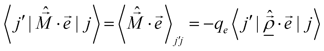
with  the expectation value of excitonic transition dipole moment for the THz field polarization
  is the relative spatial operator and in reduced notation ωj′j = ωn′m′,nm = ωj′ − ωj is the transition frequency and γj′j is the broadening. The final two-level polarizability αj′↔j = αj′j + αjj′ calculated from eqn (1) shows both resonant and antiresonant contributions, which allow a finite and real zero frequency polarizability. Fig. 1(a) displays the normalized polarizability from eqn (1) for a simulated transition resonant at 5 THz and a dephasing of γj′j = 35 ps−1,28 a typical value for CdSe NPLs. The typical pole function for the real part and the peak lineshape for the imaginary part result from the complex valued Lorentzians in eqn (1). Due to the latter, the imaginary static polarizability is zero, while the real part is finite. In the following, however, we consider typical CdSe NPLs of 4.5 monolayer (ML) thickness and 30 × 20 nm2 size.
 |
| | Fig. 1 (a and b) Normalized polarizability of a simulated transition at 5 THz according to eqn (1) and (c and d) converted mobility according to eqn (2) at 300 K (γ = 35 ps−1). Short and long dotted lines depict contributions to excitonic mobility (solid line) through different velocity descriptions of relative e- and h-motion. | |
THz experiments give insight into the (exciton) mobility μ. So to analyze experimental THz spectra, which allow to retrieve the optical (intra-particle) conductivity (σX = qenXμX, with nX the density of excitons) or dielectric function change, the question arises how the mobility μ relates to the excitonic polarizability. We propose the transformation
| |  | (2) |
for the polarizability
αj′j of a transition pair

, again with excitonic quantum numbers
n,
m and
n′,
m′, respectively. The corresponding transition frequencies are
ωj′j and
γj′j, which are the corresponding dephasing (relaxation) rate coefficients so that subsequently the mobility
μj′j is obtained, with
qe being the electron charge. Arranging the transition frequencies
ω, rate coefficients
γ and corresponding polarizabilities
α in matrices (
j′ column index,
j rows index) allows interpreting the last term of
eqn (2) as the so called Schur product of the matrix (
iωj′j +
γj′j) and the polarizability matrix
αj′j, generalized from
eqn (1). We note that the resultant
μX(
ω) is a scalar.
25
In contradiction to eqn (2), however, often in the literature, a transformation with continuous ω and a constant α0 is used29–33
As we will discuss in the second part of this paper, this transformation relies on treating an exciton intraband transition as a single damped Lorentz oscillator, driven by a monochromatic CW wave of frequency
ω, Taylor-expanded in a low frequency limit, like for microwave spectroscopy. However,
eqn (3) becomes peculiar in THz experiments, where short single cycle THz pulses with a multi THz span spectrum are used. Further,
eqn (3) allows no calculation of the static polarizability
α0 from the measured mobility, as the zero-frequency polarizability can not diverge. We show, however, that this singularity does not occur using
eqn (2).
In the following, we deduce eqn (2) and discuss the fundamental differences to eqn (3), before we deduce and discuss the latter briefly.
2.1 Response theory approach
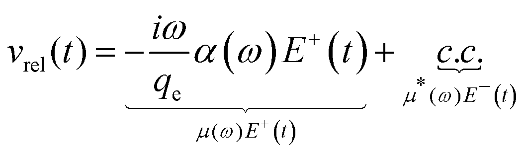
A changing dipole moment (t), caused by interaction with a THz field of polarization ![[e with combining right harpoon above (vector)]](https://www.rsc.org/images/entities/i_char_0065_20d1.gif) , induces a relative motion of electron and hole with a velocity
, induces a relative motion of electron and hole with a velocity ![[v with combining right harpoon above (vector)]](https://www.rsc.org/images/entities/i_char_0076_20d1.gif) rel.
rel.| |  | (4) |
Hence, transitions occur between states of relative motion, for which we rewrite eqn (4) in terms of a quantum mechanical matrix element representing an intraexcitonic transition  .
.| |  | (5) |
Alonso and De Vincenzo first pointed out that – in the case of a non-Hermitean operator – the temporal derivative of the spatial expectation value no longer obeys the correspondence principle through the Ehrenfest Theorem in its known form (〈v〉 = d〈x〉/dt = 〈p〉/m).34–36 Instead, it has to be extended, implementing an additional term  to read in our specific excitonic case
  . We refer to the ESI,† Section S1, for a detailed evaluation of the matrix element's time derivative. In essence, we obtain
| |  | (6) |
We Fourier transform both sides of eqn (6), exploiting the convolution relations, see the ESI,† S1:| |  | (7) |
| |  | (8) |
Dividing both sides of the Fourier transformed eqn (6) (using eqn (7) and (8)) by E(ω), we arrive at (detailed derivation in the ESI,† Section S1C)| |  | (9) |
where we implicitly assume that the αj′j entries are scalar, so that the induced polarization is in direction of the perturbing field . Again, we emphasize that each state  is associated with a tuple of quantum numbers (n, m). Under this consideration, a summation over all final states
  as well as initial states
  results in the complex exciton mobility in eqn (2). We remark that, in this linear response theory, the weak THz-probe field E(t) can have any time dependence and associated spectrum E(ω), for instance a Gaussian pulse.
2.2 Classical oscillator model
The direct ω scaling in the previously mentioned transformation formula in eqn (3) arises from an oscillator model, starting from a classical equation of charge motion:| |  | (10) |
Here, E0![[thin space (1/6-em)]](https://www.rsc.org/images/entities/char_2009.gif) cos(ωt) = E0Re[eiωt] = (E0/2)(eiωt + e−iωt) = E+(t) + E−(t) is the real (monochromatic) excitation field, mr is the reduced exciton mass, and ω0 is the electronic transition frequency. A solution to the problem can be obtained by substituting
cos(ωt) = E0Re[eiωt] = (E0/2)(eiωt + e−iωt) = E+(t) + E−(t) is the real (monochromatic) excitation field, mr is the reduced exciton mass, and ω0 is the electronic transition frequency. A solution to the problem can be obtained by substituting  and solving the differential equation for eiωt excitation.
| |  | (11) |
The solution can be found by inserting the trial function z(t) = C(ω)·eiωt, with C(ω) a complex function. Solving for C(ω) results in C(ω) = −(qeE0/mr)(ω02 − ω2 + iγω)−1. Using  = Re[z(t)] = (z(t) + z*(t))/2, with z* the complex conjugate of z, we write
| |  | (12) |
Again, employing the excitonic transition dipole moment
, we rearrange
eqn (12)| |  | (13) |
and identify the frequency-dependent polarizability
α and its complex conjugate. Using
eqn (12), we obtain the time-dependent velocity of relative motion according to

| |  | (14) |
For clarity, we factorize
eqn (14) by identifying
α from
eqn (13)| |  | (15) |
into terms with the field components
E+(
t) and
E−(
t). By identification, this directly allows retrieving
| |  | (16) |
which is used in the literature
29,30,32,33,37 without derivation. From here, often two approaches are distinguished: (i) it is assumed that – due to the bosonic nature of excitons – the 1s ground state is fully populated, implying a frequency dependent
α(
ω), however, with a resonance far from the static limit. (ii) The polarizability
α0 is constant, although stemming from multiple transitions
38 and scales linearly with
ω (
eqn (3)). In contrast to this result and similar to the derivation in
eqn (6)–(8), a convolution approach with the excitation field is necessary, as we have shown.
Eqn (3) is valid only for very special cases, discussed in the following section, while
eqn (2) is valid for all systems including multiple levels and for the entire frequency range. Two points are especially important: the
ωij scaling and the dephasing dependence, discussed in the following.
2.3 Modeling results
In this section, we compare the results of the different theoretical approaches. Fig. 1 displays frequency-dependent shapes of α and μ according to eqn (2) for an exemplary simulated transition resonant at 5 THz.
While the multiplication by i interchanges real- and imaginary parts, eqn (2) translates a finite static α0 (ω = 0) into a vanishing μ0 (ω = 0). This is similar to eqn (3), which delivers zero due to the ω scaling. However, this common property is based on completely different physical grounds: (i) in eqn (2), the extended Ehrenfest Theorem (see eqn (5) and (6)) creates a second contribution  canceling the THz absorption induced relative e–h-motion contribution
  in the low-frequency regime (Fig. 1 short and long dotted lines). (ii) Based on eqn (16), in eqn (3), however, a classically described exciton is responding linearly to a monochromatic electric field driving of frequency ω near the static limit α0 where α(ω) is quasi constant, see Fig. 1a.
In general, the analysis of the experimental THz results should be done on the mobility or conductivity (σX = qenXμX) basis. The latter should be used, if there are additional signal contributions from unbound electrons and holes (σc = qe(neμe + nhμh)).19,27,39 Here, ni, i = X, e, h is the particle density in the system. An inversion of eqn (2) to retrieve the excitonic polarizability contribution is possible if the entries of the transition frequency and relaxation matrix are known from the electronic system modeling of the nanoparticles. Otherwise, the relaxation matrix can be varied as a free modeling parameter. In contrast, eqn (3) is unphysical, as a missing real part (γj′j) in the correct transformation prefactor (iωj′j + γj′j) imposes a harsh violation of the Kramers–Kronig relations and divergence for ω = 0. Hence, it can be ruled out and our new, correct transformation should be used since the addition of γj′j allows transformation in both directions. We remark that there is always an imaginary part of α, since it can be shown that the absorption cross section of a transition relates via σabs(ω) = ω/(cε0)![[scr J, script letter J]](https://www.rsc.org/images/entities/char_e529.gif)
![[scr M, script letter M]](https://www.rsc.org/images/entities/char_e145.gif) {α(ω)}.40
{α(ω)}.40
Finally, it is remarkable that the classically explained (however, to some extent unjustified and simplified) approaches from literature emerge unconstrained from our rigorous quantum mechanical treatment. In particular, we can show (see also the ESI,† Section S1D)
| |  | (17) |
where we point out that the equation already holds for the summation of each of two resonant and antiresonant transition pairs (
j →
j′ and
j′ →
j). Our new transfer
eqn (17) has the following advantages: (i) it makes the formal quantum mechanical transformation formula approachable for experimentalists, since it allows plain
ω scaling to the somewhat simpler quantum mechanical polarizability by
eqn (1), (ii) it proves, that
ω scaling is only valid when considering the full frequency-dependent quantum mechanical polarizability summing up all possible transitions under given conditions and thus makes the constant
α0 scaling in
eqn (3) at least incomplete. (iii) We now understand, how the
ω scaling emerges from a full quantum mechanical treatment, without the need of classical mechanics. We refer to the ESI,
† Section S1D for a detailed discussion of how these expressions relate.
Besides the discussed conversion, we want to elaborate what impacts the static polarizability. Typically, it is assumed for optical pump-THz probe polarizability investigations that the photogenerated exciton resides after a short cooling time in the  ground state (GS) of relative motion.3,7,8,41,42 As a consequence, a number of dipole allowed transitions, e.g.
 , is addressed by THz-radiation, so that
  , while other transitions are dipole forbidden. That all transitions
  are dipole allowed can be verified easily using 2D hydrogenic states43 and calculating the respective dipole matrix elements. At room temperature, however, where most experiments are conducted, the exciton population distributes over the manifold of relative motion states according to Bose–Einstein statistics,44,45 see the sketch of the populations to the right of Fig. 2. As this is the case, absorption of THz-radiation does not only lead to transitions from
  , but a multitude of allowed transitions within the discrete intraexcitonic series. We note that this is supported by experimentally determined room-temperature static polarizability values of 3.1 × 10−36 C m2 V−146 and 3.0 × 10−36 C m2 V−130 for CdSe NPLs of comparable dimensions, which show comparable zero-frequency polarizability as our results from Fig. 2(a). Discarding the thermal distribution, however, the estimated DC polarizability of the excitonic system condensed into the GS only shows ∼0.18 × 10−36 C m2 V−1 (see Fig. 2(b)) a strong underestimation as compared to the experimental values. We model the 2D exciton states and the occurring intraexciton transition matrix elements as explained in the ESI,† Section S2. Fig. 2(a) shows αX resulting from all allowed transitions within the 1st to 5th shell (dark green) and all allowed transitions starting from
  only (orange). From subfigure (b), it is obvious that
  dominates the GS only polarizability. The large discrepancy between
  only and the consideration of higher final states results in missing high energy contributions with decreasing amplitude (see the ESI,† Section S3 for the treatment of a thermal distribution of initial and final states for the THz transitions).
 |
| | Fig. 2 (a) Real excitonic polarizability resulting from all possible intraexcitonic transitions (dark green) and 1s to np transition only (light green) within the 1st to 5th shell at 300 K. (b) Individual 1s → 2p, 3p, 4p and 5p contributions (γ = 35 ps−1) for ground state only population. Sketch: left – thermal population of excitons according to a Bose Einstein distribution. Subsequent allowed transitions within the discrete excitonic series. Transition dipole moments increase with decreasing energetic distance. Right – 1s → np transitions only. The full ground state (GS) population, indicated by the circle diameter, is possible at 0 K only. | |
On the other hand, the inclusion of more thermally populated initial states in (a) results in additional low energy transitions between states close to the exciton continuum, contributing to the low-frequency response (a dark green line). Although states far from the GS are weakly populated, altogether their contribution is considerable, because transition dipole moments are large for transitions between the higher, energetically close states. This is indicated also in Fig. 2 (right sketch 300 K), where the color saturation level indicates the strength of the allowed transitions.
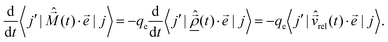
Fig. 3 compares mobilities from eqn (2), (3) and (16) for the considered NPLs, the latter two represent different conditions: (i) a static polarizability calculated from thermal distribution scaling linearly in ω (eqn (3)) and (ii) a frequency-dependent alpha, resulting only from the strong 1s → 2p transition, scaling linearly in ω as well (eqn (16)). We remark, if the results of Fig. 3 should be compared to experimental findings, the displayed intra-particle exciton mobilities have to be converted into effective medium conductivities σeff = fVξqenXμX consisting of platelets and host medium. fV is the platelet volume fraction and ξ = 2/3 + εm2/(3εp2) is the effective medium factor47 for random orientation of platelets, e.g. dispersed in solution. For toluene as a solvent (εm = 1.8548) and 2D CdSe nanoplatelets (εp = 10.249), ξ = 0.68 is obtained as the scaling factor to obtain σeff.
 |
| | Fig. 3 Real parts (a–d) and imaginary parts (e–h) of μX under varying dephasing for CdSe NPLs in a 0–30 THz window. (d and e) 0–3 THz mobility window (comparable with the yellow colored areas above) for small dephasing. | |
Here, however, as conditions may differ from experiment to experiment, we discuss in the following the complex exciton mobility instead of the conductivity in Fig. 3. Considering the imaginary part, only very close to the DC limit, the ω scaling of the static polarizability (eqn (3)) approaches the correct results (eqn (2)), as seen by comparing red and light red lines in (e–h). On the other hand, taking transitions out of the 1s ground state only into account does not describe the physical situation at room temperature reliably, where THz experiments are conducted typically.29,30,32,33,42 For CdSe NPLs for example, the dephasing is γ ∼ 35 ps−1 at room temperature,28 corresponding to the case in Fig. 3(b and f). With decreasing temperature and thereby smaller dephasing (e.g. 10 ps−1) the deviations from the correct scaling and thermal population (i.e. within the usually relevant 0–3 THz window size) become substantial, especially in the low frequency range. The assumption of a linearly growing (imaginary) mobility (constant α0) is unreasonable, also the GS only case, as the deviations from the proper (iωj′j + γj′j) scaling are considerable. Looking at the real part, a pure GS population (pale green dotted line) only leaves a vanishingly small low frequency contribution, as the low energy transitions between higher states are missing, irrespective of the different dephasing values. We remark that the real part of the mobility is zero for the constant α0 cases, while the introduction of the further necessary transitions results in a considerable mobility below 1 THz, beyond the GS only approximation. Summing up all observations, a thermal population model as well as the correct (iωj′j + γj′j) scaling have to be applied to analyze frequency-dependent THz mobility or conductivity data, while dephasing strongly impacts the resultant mobility. The latter leads to an amplitude increase at the resonances with reduced dephasing.
3 Conclusion
In summary, we have derived a transformation for excitonic polarizability into mobility, which can be applied for an in-depth analysis of THz conductivity experiments. A simple ω scaling for a constant polarizability, as suggested in the literature, is ruled out, as it neither allows calculating the real mobility nor is applicable in the typical 0–3 THz range of experiments. Furthermore, we demonstrated that the consideration of a thermal distribution of excitons and thus transitions between higher states as well as dephasing are indispensable for the analysis of room-temperature data. Dephasing influences the mobility spectra at all temperatures and has to be considered. In contrast, common approaches capture the excitonic properties only under specific conditions, e.g. zero dephasing or low temperature, which mostly do not apply. The presented results are of immediate interest e.g. for investigations on nanomaterials and their application in high bandwidth and low noise nanoelectronics or solar energy harvesting. The in-depth understanding of the exciton mobility allows for example to boost charge extraction efficiencies of solar cells, light emission performance of LEDs or solar hydrogen generation by a microscopic understanding of the THz conductivity experiments used for materials characterization.
Author contributions
M. T. Q. and A. W. A. contributed equally to this work.
Conflicts of interest
There are no conflicts to declare.
Acknowledgements
A. W. A. acknowledges funding by DFG project number AC290-2/2.
Notes and references
-
C. Kittel, Introduction to solid state physics, Wiley, 2004 Search PubMed.
- T. G. Pedersen, Solid State Commun., 2007, 141, 569–572 CrossRef CAS.
- F. Wang, J. Shan, M. Islam, I. Herman, M. Bonn and T. Heinz, Nat. Mater., 2006, 5, 861–864 CrossRef CAS PubMed.
- P. Szabó, S. Góger, J. Charry, M. R. Karimpour, D. V. Fedorov and A. Tkatchenko, Phys. Rev. Lett., 2022, 128, 070602 CrossRef PubMed.
- J. Lauth, S. Kinge and L. D. Siebbeles, Z. Phys. Chem., 2017, 231, 107–119 CrossRef CAS.
- A. Burgos-Caminal, E. Socie, M. E. F. Bouduban and J.-E. Moser, J. Phys. Chem. Lett., 2020, 11, 7692–7701 CrossRef CAS PubMed.
- R. A. Kaindl, D. Hägele, M. A. Carnahan and D. S. Chemla, Phys. Rev. B: Condens. Matter Mater. Phys., 2009, 79, 045320 CrossRef.
- R. Kaindl, D. Hägele, M. Carnahan, R. Lövenich and D. Chemla, Phys. Status Solidi B, 2003, 238, 451–454 CrossRef CAS.
- R. Huber, B. A. Schmid, Y. R. Shen, D. S. Chemla and R. A. Kaindl, Phys. Rev. Lett., 2006, 96, 017402 CrossRef PubMed.
- J. Lloyd-Hughes, H. E. Beere, D. A. Ritchie and M. B. Johnston, Phys. Rev. B: Condens. Matter Mater. Phys., 2008, 77, 125322 CrossRef.
- J. J. H. Pijpers, M. T. W. Milder, C. Delerue and M. Bonn, J. Phys. Chem. C, 2010, 114, 6318–6324 CrossRef CAS.
- R. Ulbricht, J. J. H. Pijpers, E. Groeneveld, R. Koole, C. D. M. Donega, D. Vanmaekelbergh, C. Delerue, G. Allan and M. Bonn, Nano Lett., 2012, 12, 4937–4942 CrossRef CAS PubMed.
- J. K. Gustafson, P. D. Cunningham, K. M. McCreary, B. T. Jonker and L. M. Hayden, J. Phys. Chem. C, 2019, 123, 30676–30683 CrossRef CAS.
- J. A. Spies, J. Neu, U. T. Tayvah, M. D. Capobianco, B. Pattengale, S. Ostresh and C. A. Schmuttenmaer, J. Phys. Chem. C, 2020, 124, 22335–22346 CrossRef CAS.
- H. Hempel, T. J. Savenjie, M. Stolterfoht, J. Neu, M. Failla, V. C. Paingad, P. Kužel, E. J. Heilweil, J. A. Spies, M. Schleuning, J. Zhao, D. Friedrich, K. Schwarzburg, L. D. Siebbeles, P. Dörflinger, V. Dyakonov, R. Katoh, M. J. Hong, J. G. Labram, M. Monti, E. Butler-Caddle, J. Lloyd-Hughes, M. M. Taheri, J. B. Baxter, T. J. Magnanelli, S. Luo, J. M. Cardon, S. Ardo and T. Unold, Adv. Energy Mater., 2022, 12, 2102776 CrossRef CAS.
- K. Wang, C. Chen, H. Liao, S. Wang, J. Tang, M. C. Beard and Y. Yang, J. Phys. Chem. Lett., 2019, 10, 4881–4887 CrossRef CAS PubMed.
- D. Zhao and E. E. M. Chia, Adv. Opt. Mater., 2020, 8, 1900783 CrossRef CAS.
- C. He, L. Zhu, Q. Zhao, Y. Huang, Z. Yao, W. Du, Y. He, S. Zhang and X. Xu, Adv. Opt. Mater., 2018, 6, 1800290 CrossRef.
- A. W. Achtstein, N. Owschimikow and M. T. Quick, Nanoscale, 2022, 14, 19–25 RSC.
- F. García Flórez, A. Kulkarni, L. D. A. Siebbeles and H. T. C. Stoof, Phys. Rev. B, 2019, 100, 245302 CrossRef.
- S. Ithurria, M. D. Tessier, B. Mahler, R. P. S. M. Lobo, B. Dubertret and A. L. Efros, Nat. Mater., 2011, 10, 936–941 CrossRef CAS PubMed.
- A. W. Achtstein, A. Schliwa, A. Prudnikau, M. Hardzei, M. V. Artemyev, C. Thomsen and U. Woggon, Nano Lett., 2012, 12, 3151–3157 CrossRef CAS PubMed.
- S. Ayari, M. T. Quick, N. Owschimikow, S. Christodoulou, G. H. V. Bertrand, M. Artemyev, I. Moreels, U. Woggon, S. Jaziri and A. W. Achtstein, Nanoscale, 2020, 12, 14448–14458 RSC.
- D. F. Macias-Pinilla, J. Planelles, I. Mora-Seró and J. I. Climente, J. Phys. Chem. C, 2021, 125, 15614–15622 CrossRef CAS.
-
H. Haug and S. W. Koch, Quantum Theory of the Optical and Electronic Properties of Semiconductors, World Scientiffic, 5th edn, 2009 Search PubMed.
-
K. Bonin and V. Kresin, Electric-Dipole Polarizabilities of Atoms, Molecules, and Clusters, World Scientific, 1997 Search PubMed.
- M. T. Quick, S. Ayari, N. Owschimikow, S. Jaziri and A. W. Achtstein, ACS Appl. Nano Mater., 2022, 5, 8306–8313 CrossRef CAS.
- A. W. Achtstein, S. Ayari, S. Helmrich, M. T. Quick, N. Owschimikow, S. Jaziri and U. Woggon, Nanoscale, 2020, 12, 23521–23531 RSC.
- F. García Flórez, A. Kulkarni, L. D. A. Siebbeles and H. T. C. Stoof, Phys. Rev. B, 2019, 100, 245302 CrossRef.
- R. Tomar, A. Kulkarni, K. Chen, S. Singh, D. van Thourhout, J. M. Hodgkiss, L. D. Siebbeles, Z. Hens and P. Geiregat, J. Phys. Chem. C, 2019, 123, 9640–9650 CrossRef CAS.
- P. D. Cunningham, A. T. Hanbicki, T. L. Reinecke, K. M. McCreary and B. T. Jonker, Nat. Commun., 2019, 10, 5539 CrossRef CAS PubMed.
- E. Hendry, M. Koeberg, J. M. Schins, H. K. Nienhuys, V. Sundström, L. D. A. Siebbeles and M. Bonn, Phys. Rev. B: Condens. Matter Mater. Phys., 2005, 71, 125201 CrossRef.
- J. Lauth, A. Kulkarni, F. C. M. Spoor, N. Renaud, F. C. Grozema, A. J. Houtepen, J. M. Schins, S. Kinge and L. D. A. Siebbeles, J. Phys. Chem. Lett., 2016, 7, 4191–4196 CrossRef CAS PubMed.
- V. Alonso, S. De Vincenzo and L. Gonzalez-Diaz, Il Nuovo Cimento B, 2000, 115, 155–164 Search PubMed.
- S. De Vincenco, Rev. Bras. Ensino Fis., 2013, 35, 2308 Search PubMed.
- M. T. Quick, Q. Wach, N. Owschimikow and A. W. Achtstein, Adv. Photonics Res., 2022, 3, 2200243 CrossRef.
- P. D. Cunningham, IEEE Trans. Terahertz Sci. Technol., 2013, 3, 494–498 CAS.
- E. L. Crowell and M. G. Kuzyk, J. Opt. Soc. Am. B, 2018, 35, 2412 CrossRef CAS.
- M. T. Quick, N. Owschimikow and A. W. Achtstein, J. Phys. Chem. Lett., 2021, 12, 7688–7695 CrossRef CAS PubMed.
-
R. W. Boyd, Nonlinear Optics, Academic Press, 2008 Search PubMed.
- J. Lauth, M. Failla, E. Klein, C. Klinke, S. Kinge and L. D. A. Siebbeles, Nanoscale, 2019, 11, 21569–21576 RSC.
- G. L. Dakovski, S. Lan, C. Xia and J. Shan, J. Phys. Chem. C, 2007, 111, 5904–5908 CrossRef CAS.
-
B. K. Basu, Theory of Optical Processes in Semiconductors, Oxford Univ. Press, Oxford, 1997 Search PubMed.
-
S. A. Moskalenko and D. W. Snoke, Bose-Einstein Condensation of Excitons and Biexcitons: And Coherent Nonlinear Optics with Excitons, Cambridge University Press, 2000 Search PubMed.
-
J. Shah, Ultrafast Spectroscopy of Semiconductors and Semiconductor Nanostructures, Springer, 1999 Search PubMed.
- R. Scott, A. W. Achtstein, A. V. Prudnikau, A. Antanovich, L. D. A. Siebbeles, M. Artemyev and U. Woggon, Nano Lett., 2016, 16, 6576–6583 CrossRef CAS PubMed.
- L. T. Kunneman, J. M. Schins, S. Pedetti, H. Heuclin, F. C. Grozema, A. J. Houtepen, B. Dubertret and L. D. A. Siebbeles, Nano Lett., 2014, 14, 7039–7045 CrossRef CAS PubMed.
-
S. Nashima, R. Nishimura and M. Hosoda, 37th International Conference on Infrared, Millimeter, and Terahertz Waves, 2012, pp. 1–2 Search PubMed.
-
J. Singh, Physics of Semiconductors and Their Heterostructures, McGraw-Hill, 1992 Search PubMed.
|
| This journal is © the Owner Societies 2023 |
Click here to see how this site uses Cookies. View our privacy policy here. 
 Open Access Article
 This Open Access Article is licensed under a
  *a
*a
 , not to be confused with the density matrix ρ used in the ESI†),23 whereas the center of mass (COM) wavefunction (coordinate R) is unaffected by the THz field. A separation of COM and relative coordinates is justified by the much larger lateral extent of the nanoplatelet as compared to the ∼1.6 nm Bohr radius of the correlated excitons.23 The THz radiation transition dipole moment
  is described by transitions between discrete exciton states of relative motion
  and
and  , each of them is associated with a relative coordinate
  . n and m are the main and angular momentum quantum numbers for the considered correlated exciton series in our 2D semiconductor platelets, respectively.25 Hats imply operators, like for
  and
and  . Each transition from
  is characterized by the frequency-dependent polarizability tensor αj′j(ω), with
  . Considering only one (e.g. the lowest intra-excitonic transition) at first, the scalar polarizability of the resulting two-level transition (of occupation probability b) for weak polarization fields and without rotating wave approximation is26,27
 the expectation value of excitonic transition dipole moment for the THz field polarization
  is the relative spatial operator and in reduced notation ωj′j = ωn′m′,nm = ωj′ − ωj is the transition frequency and γj′j is the broadening. The final two-level polarizability αj′↔j = αj′j + αjj′ calculated from eqn (1) shows both resonant and antiresonant contributions, which allow a finite and real zero frequency polarizability. Fig. 1(a) displays the normalized polarizability from eqn (1) for a simulated transition resonant at 5 THz and a dephasing of γj′j = 35 ps−1,28 a typical value for CdSe NPLs. The typical pole function for the real part and the peak lineshape for the imaginary part result from the complex valued Lorentzians in eqn (1). Due to the latter, the imaginary static polarizability is zero, while the real part is finite. In the following, however, we consider typical CdSe NPLs of 4.5 monolayer (ML) thickness and 30 × 20 nm2 size.


 , again with excitonic quantum numbers n, m and n′, m′, respectively. The corresponding transition frequencies are ωj′j and γj′j, which are the corresponding dephasing (relaxation) rate coefficients so that subsequently the mobility μj′j is obtained, with qe being the electron charge. Arranging the transition frequencies ω, rate coefficients γ and corresponding polarizabilities α in matrices (j′ column index, j rows index) allows interpreting the last term of eqn (2) as the so called Schur product of the matrix (iωj′j + γj′j) and the polarizability matrix αj′j, generalized from eqn (1). We note that the resultant μX(ω) is a scalar.25

 .
.
 to read in our specific excitonic case
  . We refer to the ESI,† Section S1, for a detailed evaluation of the matrix element's time derivative. In essence, we obtain


 is associated with a tuple of quantum numbers (n, m). Under this consideration, a summation over all final states
  as well as initial states
  results in the complex exciton mobility in eqn (2). We remark that, in this linear response theory, the weak THz-probe field E(t) can have any time dependence and associated spectrum E(ω), for instance a Gaussian pulse.

 and solving the differential equation for eiωt excitation.
 = Re[z(t)] = (z(t) + z*(t))/2, with z* the complex conjugate of z, we write
 , we rearrange eqn (12)


 canceling the THz absorption induced relative e–h-motion contribution
  in the low-frequency regime (Fig. 1 short and long dotted lines). (ii) Based on eqn (16), in eqn (3), however, a classically described exciton is responding linearly to a monochromatic electric field driving of frequency ω near the static limit α0 where α(ω) is quasi constant, see Fig. 1a.
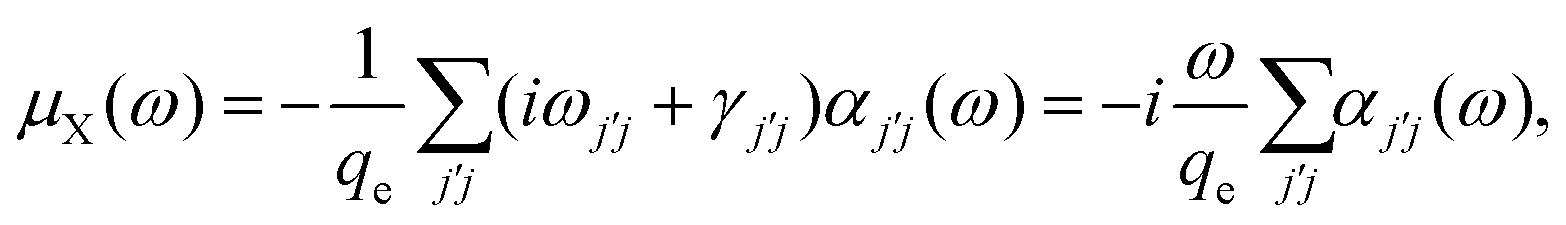
 ground state (GS) of relative motion.3,7,8,41,42 As a consequence, a number of dipole allowed transitions, e.g.
 , is addressed by THz-radiation, so that
  , while other transitions are dipole forbidden. That all transitions
  are dipole allowed can be verified easily using 2D hydrogenic states43 and calculating the respective dipole matrix elements. At room temperature, however, where most experiments are conducted, the exciton population distributes over the manifold of relative motion states according to Bose–Einstein statistics,44,45 see the sketch of the populations to the right of Fig. 2. As this is the case, absorption of THz-radiation does not only lead to transitions from
  , but a multitude of allowed transitions within the discrete intraexcitonic series. We note that this is supported by experimentally determined room-temperature static polarizability values of 3.1 × 10−36 C m2 V−1
 only (orange). From subfigure (b), it is obvious that
  dominates the GS only polarizability. The large discrepancy between
  only and the consideration of higher final states results in missing high energy contributions with decreasing amplitude (see the ESI,† Section S3 for the treatment of a thermal distribution of initial and final states for the THz transitions).
