A novel low-cost plug-and-play multi-spectral LED based fluorometer, with application to chlorophyll detection

Abstract

In this paper a novel low-cost multi-spectral optical fluorometer is presented and evaluated. The device uses a range of LEDs in the blue and violet regions of the electromagnetic spectrum and a mini-spectrometer to detect the emitted fluorescence in the UV to IR spectrum region. Custom built electronics and software were designed to control the system and the components were housed in bespoke 3D printed parts. A number of known fluorophores were tested to determine the capabilities of the fluorometer. Application of the device is demonstrated for the detection of chlorophyll a (Chl a) from laboratory grown algae and from environmental samples while analytical performance is established using both in vivo and extracted Chl a fluorescence and by comparison with a benchtop fluorometer.

---

Introduction

With increasing environmental pressure due to global climate change, increases in global population and the need for sustainable obtained resources, water resources management is critical.¹ Sensors and instrumentation play a key role in water management, and are becoming smaller, smarter and more economical.^2–5 Optical based sensors are receiving great interest due recent advances in photonics and the ability to work in harsh environments.^2,6 In aquatic environments, fluorescence based spectroscopy is a common technique used for detection and quantification of chlorophyll (Chl a),^4,7,8 petroleum compounds,⁹ fDOM (fluorescent dissolved organic matter),^10,11 tryptophan,¹² algal populations^13–15 and faecal indicator bacteria.^16,17 Chlorophyll measurement in aquatic systems is an indicator of phytoplankton biomass and primary production in response to nutrients and light availability. Excessive enrichment of waters with nutrients causes eutrophication, harmful algal blooms and loss in species diversity.^18,19 Analysis and monitoring of Chl a is critical in determining the trophic status of water bodies,²⁰ time-series trends²¹ and where applicable reactive management. For example, the Marine Water Framework Directive (MWFD) aims to achieve ‘good environmental status of the EU's marine waters’ and the Water Framework Directive aims to achieve ‘good ecological status’.²² Chlorophyll fluorescence has been primarily measured in vitro after extraction in acetone and has led to the development of standard methods.²³ Today, measurements are routinely carried in vivo using in situ submersible fluorometers⁷ and remotely using satellites and aircraft. Naturally, chlorophyll occurs in several distinct forms, with a and b being the major types found in higher plants and green algae. Combined, chlorophyll and other cellular components and pigments inside phytoplankton cells have a maximum absorption near 440 nm and maximum fluorescence at 685 nm.^24,25 These excitation/emission pairs or similar have been used historically for chlorophyll measurements.²⁶

Fluorescent molecules absorb energy in the form of light, and after undergoing a non-radiative process, light of a longer wavelengths is emitted as fluorescence.²⁷ This makes fluorescence a very sensitive and attractive techniques as the measurements are carried in the absence of incident light. For the detection of fluorescence, monochromators, such as a diffraction grating or optical filters are typically used to select the desired emission wavelength. Once filtered this light is typically directed towards a photo-multiplier tube (PMT) for detection. These systems for fluorescence detection are typically rather bulky and not suitable for in situ or continuous monitoring of local events. Thus the majority of environmental sensors, either for fluorescence or scatter measurements employ photodiodes as photodetectors and light emitting diodes (LED) as light sources.⁷ Selectivity to target analytes is thus achieved through the use of LEDs with narrow bandwidth emissions, laser diodes and optical filters which in general block or reduce the leaching of incident light into the photodiodes.^16,28–33 In the race to miniaturisation and field application a range of photodetectors have been demonstrated in the literature for different applications and include: PMTs^4,34,35 which although have excellent sensitivity require higher voltages to operate, camera sensors,^36–38 PDs^16,28,39 and CdS phototransistors.^3,33

Due to the low cost, small size and improved performance these optical components have accelerated the development of in situ fluorometers. However, limitations still exist due to the complex composition of environmental waters and the overlapping of absorption or emission spectra associated with the presence of different optically active compounds.^11,40 While PDs and PMTs provide poor spectral resolution, array detectors provide multi-spectral resolution which in turn captures multiple fluorescence emission bands associated with the presence of different constituents. Thus the higher resolution enables spectral deconvolution and the assigning of emission peaks to environmental constituents. Miniaturised spectrometers now exist to enable the fabrication of low-cost portable sensors with a recent demonstration for the use of the Hamamatsu C12880MA spectrometer chip for absorbance measurements.³⁸

In this context, a novel plug-and-play LED board and miniaturised spectrometer system was designed and evaluated to detect and quantify in vivo fluorescence associated with Chl a. Initial performance was investigated with fluorescent chemical standards. System benchmarking was carried out against extracted Chl a reference measurements with laboratory cultured algae. Analysis of environmental samples was used to demonstrate system capabilities for in vivo Chl a detection and application to in situ monitoring.

Experimental

Fluorometer design and construction

Bill of materials. A bill of materials detailing the optical and electronic components and associated cost is presented in Table 1.

Table 1 Bill of materials^a

	Component	Part number	Supplier	Quantity	Unit cost (€)	Total cost (€)
a PCB-printed circuit board.
Optical	CMOS, photodetector	C12880MA	Hamamatsu Photonics, UK	1	200	200
	Colimitation lens	36689	Edmund Optics, UK	1	94.50	94.50
	Plano-convex lens	48668	Edmund Optics, UK	1	83.00	83.00
	Lens tube	SM1L03	ThorLabs, UK	1	11.95	11.95
	Threaded 30 mm cage plate	CP33/M	ThorLabs, UK	1	17.35	17.35
	360 nm LED (B1)	ATS2012UV365	Mouser Electronics, Ireland	1	2.19	2.19
	380 nm LED (B2)	ATS2012UV385	Mouser Electronics, Ireland	1	1.56	1.56
	430 nm LED (B3)	KP-2012MBC	Farnell, Ireland	1	0.86	0.86
Electronic	Teensy 3.2 microcontroller	DEV-13736	Digikey, Ireland	1	18.05	18.05
	5 V LDO voltage regulator	L7805ACD2T-TR	Digikey, Ireland	1	0.49	0.49
	LED driver	TLC59116FIPWR	Digikey, Ireland	1	1.92	1.92
Custom PCBs	Control board	—	Beta Layout, Ireland	1	25.70	25.70
	LED mounting board	—	Beta layout, Ireland	1	14.95	14.95
	CMOS mounting board	—	Beta Layout, Ireland	1	8.107	8.11
				Total		480.62

---

System overview. Fig. 1b shows a schematic representation of the overall final system level components of the sensor. The sensor is controlled by a Teensy 3.2 microcontroller (MCU) powered by a 10 V power supply using a linear drop out voltage regulator (L7805ACD2T-TR) to provide 5 V. The Teensy was mounted to a custom-built electronics board and connected via USB to a laptop. Control software was uploaded to the Teensy that allowed serial commands to be sent from the laptop to the Teensy enabling the user to control the various electronic elements such as the LEDs and mini-spectrometer. A simple user interface was developed to allow the user to send these serial commands to the Teensy. A current control chip regulated the amount of current supplied to each LED to 20 mA, regardless of operating voltage required to turn on each LED. The MCU receives data collected by the spectrometer and relays that data back to the laptop for analysis.

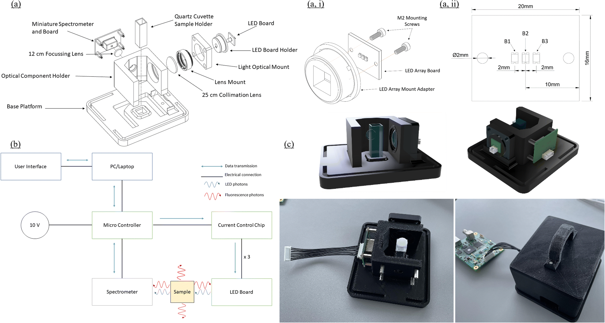Fig. 1 System design and fabrication showing the assembled plug & play benchtop optical testing prototype; (a) exploded view showing physical and optical system components and assembly; (a, i) CAD model of LED array adaptor; (a, ii) CAD model for LED array printed circuit board (PCB); (b) electronic design – system level components of the instrument, showing how the various components are connected electrically and how signals are sent between the various components; (c) 3D render (top) and 3D printed system and electronic boards (bottom).

Enclosure design iterations were carried out in SolidWorks (Fig. 1c) while the assembly parts were FDM (fused deposition modelling) 3D printed from PLA (polyacetic acid) filament using the Lulzbot Taz63D printer (Fig. 1c).

Optical design. An exploded view of the components used is shown in Fig. 1a together with a top-down view of the optical detection configuration. The illumination setup consisted of 25 cm UV fused silica plano-convex lens with a focal length of 25 mm used to collimate the light emitted from the LEDs. The lens was mounted in a ThorLabs SM1L03 stackable lens tube and held in place using a ThorLabs CP33/M threaded optical mount. The LEDs were mounted on a custom-built electronics board that was adapted for both through hole (TO) and surface mount (SMD) LEDs. When TO LEDs were used the board was held in place using a ThorLabs S1LEDM threaded mount for LEDs that was attached to the threaded optical mount, otherwise for surface mount (SMD) LEDs a custom-built LED board was used and held in place with screws (Fig. 1a(i) and a(ii)). Manufacturer provided details of the used LEDs are shown in Table 2.

Table 2 SMD LEDs used in this study

LED	Dimensions (L × W × T)	Radiant flux (mW)	FWHM (nm)
B1 (λ = 360 nm)	2 × 1.5 × 0.75	13	10
B2 (λ = 380 nm)	2 × 1.5 × 0.75	16	12
B3 (λ = 430 nm)	2 × 1.2 × 1.1	8	60

---

To detect the fluorescence emitted from the sample a 1.27 cm UV fused silica plano-convex lens with a 10 mm focal length was used to focus light onto the entrance slit of a Hamamatsu C12880MA mini-spectrometer. The mini-spectrometer has a spectral response range between 340 and 850 nm with a typical resolution of 12 nm (FWHM).

Light incident on the entrance slit of the spectrometer is passed to a reflective concave blazed grating. The light is reflected from the grating onto a high-sensitivity CMOS (complementary metal oxide semiconductor) linear image sensor with 288 pixels each corresponding to a particular wavelength, given by

λ = A₀ + B₁n + B₂n² + B₃n³ + B₄n⁴ + B₅n⁵

where, A₀, B₁, B₂, B₃, B₄ and B₅, are empirically measured constants specific to each spectrometer and n is the pixel number. The integration time of the spectrometer could be controlled and set using serial commands from the user interface, ranging from 11 μs–4 s. The integration time controls the length of time that the detector of spectrometer is allowed to collect photons before sending the accumulated charge to an analogue-to-digital (A/D) converter, weaker signals have longer integration times, while more intense signals required shorter integration times. The integration time was established at the start of each experiment by adjusting the integration time such that the intensity of the strongest signal under investigation was approximately 90% of the maximum and kept constant throughout the experiment.

System control and electronic design. A Teensy 3.2 is used as a MCU and was sourced from Digi-Key Electronics Inc., Ireland. This MCU has superior performance with an ARM Cortex-M4 MCU chip that can run at 72 MHz. In addition to the operational speeds, the MCU also possesses a high resolution analog to digital converter (ADC) which allows up to 16 bit resolution. The LED control circuitry uses a dedicated LED driver IC (TLC59116FIPWR Texas Instruments sourced from Digi-Key Electronics Inc.) which is capable of driving 16 separate channels with a regulated current set by an external resistor value and can be controlled by the MCU over I²C digital protocol which reduces the required output pins from the MCU. The IC can regulate the current consistently to keep the output intensity of the LEDs stable without variation from external factors such as temperature⁴¹ and can also output a pulse width modulated (PWM) signal to provide high frequency switch of the LEDs for dimming and power saving purposes. The IC manages the PWM signal automatically which allows the MCU to conduct other tasks or go into sleep mode, if necessary, which also reduces power consumption.

Proof of concept qualitative experiments

Initially, three high concentration solutions of quinine sulphate (Sigma-Aldrich, Ireland), extracted Chl a and cyan fluorescent protein (CFP) (Fisher Scientific, Ireland) were used for screening system application. Sample cells were 3.5 mL (10 × 10 mm) and UV quartz cuvettes, equipped with a Teflon stopper (Hellma Analytics). An appropriate integration time for each fluorophore was established by turning each LED on and adjusting the integration time until the peak of each fluorescence signal reached approximately 80–90% of the maximum signal. This ensured a high dynamic range without detector saturation.

Analytical performance with laboratory standards

The analytical performance of the device was assessed with laboratory prepared standards of Basic Blue 3 dye (BB3), Sigma-Aldrich, Ireland and comparison with a Jasco FP-8300 benchtop fluorometer.

Performance evaluation with algae cultures

Laboratory grown algae were used to determine the fluorometers capabilities to detect chlorophyll fluorescence. The diatom species Nitzschia ovalis (SAMS Limited, Scotland) was selected and cultured in filtered artificial seawater water (0.45 μm) supplemented with nutrients to make Guillard's F/2 + Si medium.⁴² The cultures were grown in batch growth system in 5 L Pyrex bottles (15–23 °C, 12 : 12 light : dark, continuous light of 65 μmol m⁻² s⁻¹). The concentration of biomass was calculated by determining the concentration of Chl a in 25 mL aliquots that were filtered at low pressure (700 mb) through GF/F glass fibre filters (Whatman GF/F, pore size 0.7 μm) kept in the dark at −20 °C for 12 hours. Subsequently, 8 mL of 90% (v/v) acetone was added to each 25 mL filtered aliquot, followed by sonication in an ultrasound bath for 5 min. Extraction was carried out in the dark at 4 °C for at least three hours following centrifugation (5000 rpm, 10 minutes) and recovery of the supernatant. Absorbance was read at 665 nm and 750 nm in a Shimadzu UV-1800 UV-Vis double beam spectrophotometer allowing the calculation of Chl a concentration as outlined in ref. 43 and conversion to μg L⁻¹ concentrations.

Environmental case study

Environmental samples were used to determine if it was possible for the sensor to be used for in vivo fluorescence. Samples were collected from Dublin Harbour and can be classified as brackish. Sample were analysed untreated on the bench-top system, with fluorescence scans collected for all three LEDs.

Results and discussion

LED evaluation

The normalized spectrum of each LED recorded by the mini-spectrometer and a commercial spectrometer, Maya 2000 PRO Series, Ocean Optics Inc., US is shown in Fig. 2. LEDs B1 and B2 have narrow band emissions with a FWHM (full width at half maximum) of 14 nm and 19 nm respectively as recorded on the mini spectrometer and 9 nm and 18 nm on the Maya spectrometer. B3 on the other hand has a much broader and asymmetrical spectrum than the other LEDs with a FWHM of 60 nm recorded on the mini-spectrometer and 58 nm on the Maya spectrometer. Overall, the LEDs cover a large portion of the blue and violet portions of the visible and near UV region of the spectrum making them good candidates for inducing fluorescence in fluorophores with excitation energies in this region. In particular, the LEDs were selected to excite Chl a and maximise light absorption but also to limit the leaching of scatter light into the photodetector at higher wavelengths (Fig. 2).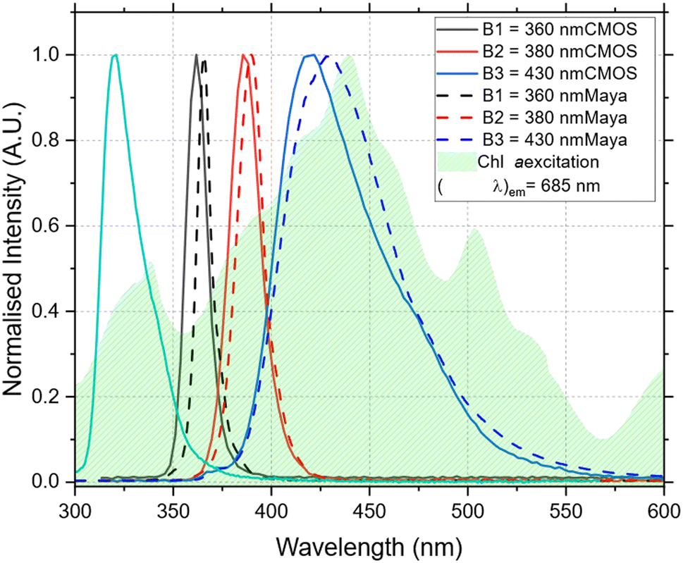

Fig. 2 Spectrum of each LED used in this study as recorded on the Hamamatsu mini-spectrometer and the Ocean Optics Maya 2000 PRO Series spectrometer. Overlayed is the in vivo excitation spectrum of cultured diatomic algae (λ_em = 685 nm).

Proof of concept qualitative experiments

Fig. 3 shows the recorded spectrum of each of the proof of concept fluorophores, with an inlay of the visible fluorescence. It was possible using each LED to induce fluorescence in each of the fluorophores tested. Fig. 3a shows the signal recorded for each LED using quinine sulfate. The fluorescence from the fluorophore was visible to the eye, and it was also possible to record the fluorescence emitted from the fluorophore and spectrally resolve it using the mini-spectrometer. Quinine sulfate is a broadband fluorescence emitter, fluorescing between approximately 400–600 nm. As such there was some overlap between the LED signal and fluorescence signal for LEDs B1 and B2, while for LED B3 the LED and fluorescence signal combine together making it not possible to fully spectrally resolve the two signals, although it was still possible to see the fluorescence with the naked eye. Fig. 3b shows the fluorescence and spectrum recorded for each LED using CFP. Again in all cases fluorescence was visible seen using as three LEDs. For LED B3 it was once again not possible to spatially resolve the fluorescence signal from the LED signal, however using B1 and B2 there was a small overlap between the LED and fluorescence spectrum, there was sufficient resolution to spectrally resolve the two signals. CFP is a broadband fluorescent maker with a fluorescence spectrum between 410 and 500 nm (FWHM) peaking at 485 nm typically used as a biological marker for physiological processes, visualizing protein localization and detecting transgenic expression in vivo. Fig. 3c shows visually the fluorescence signal from the diatom algae solution and the fluorescence signal recorded for each LED. The chlorophyll sample is a broad emitter, with fluorescence from 625–725 nm. The signal has three peaks at 640 nm, 680 nm and 720 nm with the peak at 640 nm associated with Chl b and the peaks at 680 nm and 720 nm associated with Chl a. As the fluorescence was far from the LED signals it was possible to fully resolve the fluorescence signal from the LED signals. The signal detected was strongest for the blue LEDs (B1, B2 and B3) and much weaker for the UV LEDs (UV1 and UV2) due to limitations in how high the integration time could be set using the Hamamatsu software, set at 1 s. For later experiments, custom built software was written that allowed for longer integrations times up to typically 4 s, allowing weaker signals to be detected.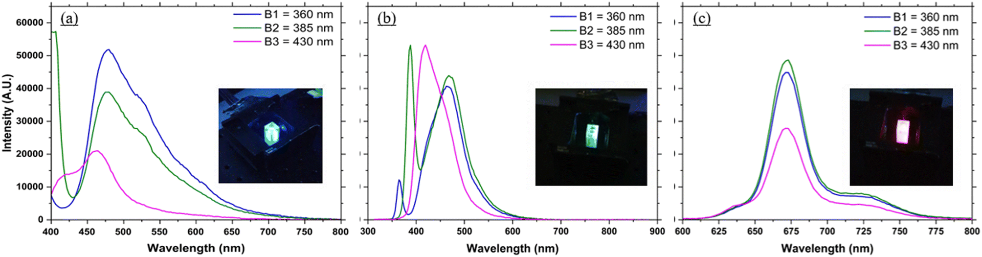

Fig. 3 (a) Quinine sulphate fluorescence spectrum recorded for each LED with an inlay of the visual fluorescence; (b) cyan fluorescent protein fluorescence spectrum as recorded for each LED with an inlay of the visible fluorescence; (c) Chl a fluorescence spectrum as recorded for each LED with an inlay of the visible fluorescence.

Analytical performance with laboratory standards

Fluorometers that measure in vivo fluorescence rely on analytical standards for calibration and quality control.⁴⁴ This approach is used to ensure reproducibility by using a stable analytical grade standard. Once the devices are calibrated to a given standard, the response can be converted to equivalent standard concentration and conversion factors can be used to infer Chl a concentration from in vivo Chl a measurements.⁴⁵ Fluorometers relying on in vivo measurements, target fluorescence emitted by Chl a molecules in photosystem II, for which the peak fluorescence emission is approx. 685 nm, although not all Chl a present is in photosystem II.⁴⁵ Standard stability and excitation/emission overlap with Chl a is thus critical in selecting a suitable standard.⁴⁴ For this reason and high solubility in water, Basic Blue 3 (BB3) was selected to benchmark the performance of the fluorometer developed here against a commercial benchtop fluorometer. Serial dilutions of BB3 in the 0–1 mg L⁻¹ range were used to collect emission scans on both instruments (Fig. 4a and b) and develop calibration curves (Fig. 4c and d). This BB3 concentration range and the fluorescence emitted was determined previously, to correspond to the expected fluorescence of Chl a in the 0.01 to 10 μg L⁻¹ range.^45,46 The benchtop fluorometer was set to the highest sensitivity setting available while the fluorometer developed here used a 2 s integration time. This integration time was optimised to maximise the dynamic range of the instrument and reduce signal-to-noise ratio. While all the BB3 dilutions were successfully detected on the benchtop fluorometer, the CMOS based fluorometer could not detect the dilutions in the low range (i.e. 0.01, 0.02 and 0.05 mg L⁻¹), Fig. 4, due to a higher signal-to-noise ratio. The calibration curve was thus constructed using the dilutions in the 0.1–1 mg L⁻¹ range. To determine the precision and accuracy of the CMOS based fluorometer, a known concentration of BB3 (0.75 mg L⁻¹) was run 10 times on both instruments (Fig. 4e). Using the developed calibration curves, each run was converted to BB3 concentration (mg L⁻¹). The average concentration was found to be 0.72 ± 0.022 for this device and 0.78 ± 0.0018 for the Jasco fluorometer with a % RSD of 3.004 and 0.23 respectively (Fig. 4f). Although the Jasco fluorometer demonstrates a higher precision, the % RSD showed by the CMOS fluorometer is within the 5% margin of error acceptable for sensors with environmental applications.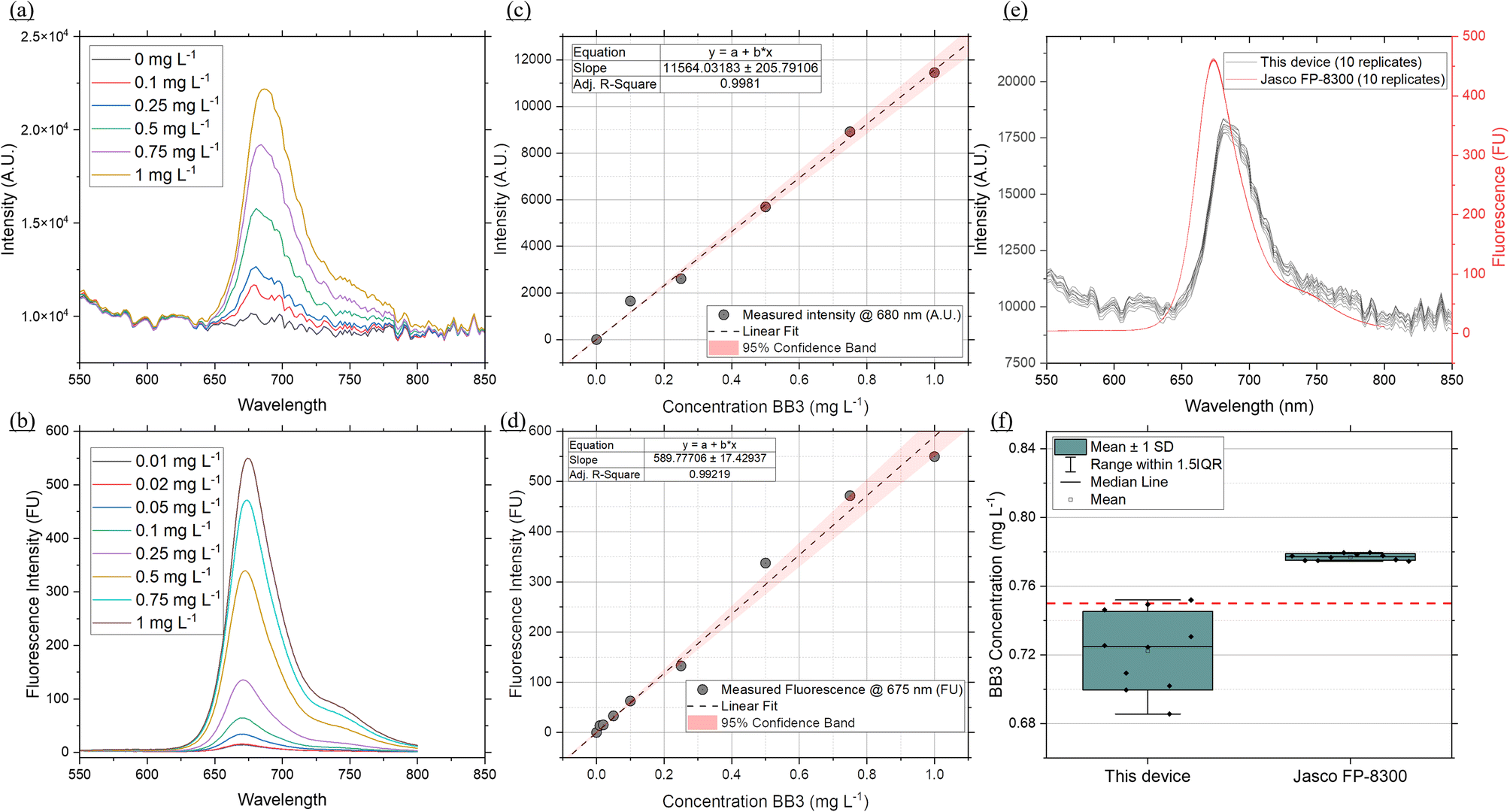

Fig. 4 Analytical performance with Basic Blue 3 dye (BB3). Emission spectra of serial dilutions of BB3 measured on (a) this device and on (b) the Jasco FP-8300 benchtop fluorometer. Calibration curves for BB3 on (c) this device (λ_em = 680 nm) and (d) on the Jasco FP-8300 (λ_em = 675 nm). (e) Ten replica scans (emission spectra) of the same concentration of BB3 (0.75 mg L⁻¹) on both instruments. (f) Box plots following conversion to BB3 (mg L⁻¹) of the 10 replica scans on both instruments, showing precision (mean ± 1 SD) and accuracy (dashed red horizontal line positioned at 0.75 mg L⁻¹) of the two devices. In (a), (c) and (e) an integration time of 2 s was used to collect the emission spectra using LED B2 (λ_max = 380 nm), in (b), (d) and (e) the sensitivity of the instrument was set to high, and slit widths for both the excitation and emission monochromators were set to 5 nm.

Application to extracted Chl a

Fig. 5a shows a sample of the Chl a spectrum using different concentrations of Chl a extracted in acetone using LED B2 (λ = 380 nm). For each of the three LEDs used in this work it was possible to detect a fluorescence signal for Chl a concentrations between 1 and 20 μg L⁻¹, with LED B2 achieving the highest signal for each concentration and LED B3 (λ = 430 nm) recording the lowest signal intensity.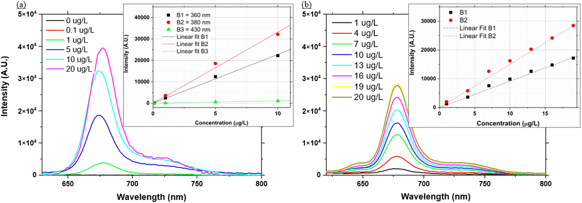

Fig. 5 (a) Fluorescence spectra of extracted Chl a in acetone using LED B2 (λ = 380 nm). Chl a was extracted from laboratory cultures of diatom species Nitzschia ovalis and quantified as described in the Experimental section; inset in (a) calibration curve for each LED with extracted Chl a in acetone using the peak fluorescence emission at 675 nm; (b) fluorescence spectra recorded using LED B2 (λ = 380 nm) of serial dilutions of laboratory drown diatom cultures; inset in (b) calibration curve between in vivo fluorescence and the diatom concentrations expressed as Chl a (μg L⁻¹) following extraction for LEDs B1 and B2. In both (a) and (b) the Chl a concentrations were determined as described in the Experimental section.

A calibration curve for each LED response was created by taking the peak of the fluorescence signal at 675 nm as recorded by the mini-spectrometer (Fig. 5a, Table 3). Due to the redshift in the fluorescence signal at 20 μg L⁻¹ it was excluded from the calibration.

Table 3 Calibration slope and R² values for acetone extracted Chl a and in vivo Chl a from cultured diatom species Nitzschia ovalis^a

LED	Extracted Chl a		In vivo Chl a
	Slope	R ^2	Slope	R ^2
a ND-not determined.
B1 (λ = 360 nm)	2248.1	0.997	878.39	0.991
B2 (λ = 380 nm)	3265.3	0.994	1498.4	0.995
B3 (λ = 430 nm)	115.03	0.991	ND	ND

---

In vivo application

Fig. 5b shows a sample of the spectra recorded using LED B2 of the diatom algae. Unlike the previous section these spectra were recorded in vivo. The measured response is widely used in environmental sensors as a proxy for Chl a concentration.⁴⁵

Fluorescence was successfully detected throughout the diatom algae concentrations with all the LEDs. LED B3 however showed the least change with increasing concentrations and was excluded from the calibration. Collected emission scans for LED B2 and calibration curves for LEDs B1 and B2 are presented in Fig. 5b while the calibration coefficients are presented in Table 3. Similarly to the extracted Chl a, LED B2 was the most sensitive to changes in concentration. Globally, Chl a concentrations range from 0.01 to 10 μg L⁻¹.^45,46 In terms of analytical performance, the system can target and successfully quantify Chl a at environmental concentrations for both in vivo measurements and combined acetone extraction.

Application to environmental samples

An example of the recorded fluorescence emission spectrum collected for environmental sample is shown in Fig. 6, between 400 and 850 nm for LEDs B1 and B2. No fluorescence signal was detected for B3, thus it is not shown. Using the calibration curves developed in the previous section it was possible to calculate the Chl a concentration by dividing the fluorescence signal peak by the slope of the calibration curve. Using the in vivo calibration curves developed with laboratory grown diatoms (Fig. 5b, Table 3) a concentration of 3.05 μg L⁻¹ was calculated for LED B1 and 3.25 μg L⁻¹ for LED B2 respectively. The Chl a concentration in the sample, following the standard method using filtration and acetone extraction was found to be 2.16 ± 0.24. Such discrepancy is expected as slope coefficients used are for in vivo Chl a fluorescence determined with laboratory cultures are expected to be different from environmental mixed populations. In general, the calibration of fluorimeters is carried out on site specific samples due to the large natural variability in the relationship between in situ fluorescence and extracted Chl a concentrations. Globally, the slope factor can range from 1 in the Arabian Sea region to greater than 6 in the Southern Ocean province, south of New Zeeland.⁴⁵ With the two sources of uncertainty when measuring in vivo being the variability in the Chl a specific absorption⁴⁷ and the variability in the fluorescence quantum yield.⁴⁶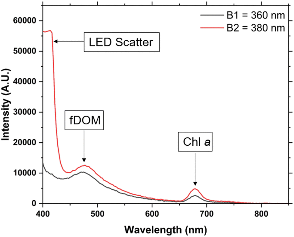

Fig. 6 Example of fluorescence spectra recorded using LEDs B1 (360 nm) and B2 (380 nm) from an environmental sample. Fluorescence from Chl a is detected between 650 and 700 nm indicating the presence of algal species in the water. In addition to the Chl a signal an unknown fluorescence signal, believed to be fDOM was also observed between 450 and 600 nm.

The set-up while not as sophisticated as devices mentioned in the Introduction section was still consistently able to induce and detect fluorescence from all samples tested, and does however solve some issues presented such as costing, reliability and overall footprint, potentially allowing in situ real time monitoring of environmental events and changes over time. Algal species for example are a vital component of aquatic marine life, serving as the basis of the oceanic food chain. As a species, their environment is threatened by global warming and climate change, and therefore monitoring their levels in oceanic environments may be an important warning mechanism while tracking the impacts of climate change. Should a suitable housing environment be developed this technology may be deployable in marine environments to monitor changes in algal populations at a relatively low-cost.

The experimental work in this work showed that it was possible to detect fluorescence produced by Chl a samples at expected environmental concentrations and using the calibration curves quantify those values, making this technology a potentially vital tool for environmental monitoring. Detection capabilities within the μg L⁻¹ are essential for real-world application, and similar devices have achieved this range using PMTs^4,48 and PDs.²⁸ The CMOS mini-spectrometer however has a spectral response range between 340 and 850 nm and a 12 nm spectral resolution. These key features enable spectral deconvolution of overlapping optical signatures and critically, detection of other optical targets within this range. Furthermore the compact, small design of the CMOS mini-spectrometer enables integration into submersible, in situ devices where size of electronic components is critical. The C12880MA chip employs a nano-printed reflective concave blazed grating which minimizes the light path and enables the realisation of small, compact detectors. By comparison, a longer optical path length is required when diffraction gratings are used in conjunction with CMOS based cameras.³⁶ The use of LEDs means that the set-up can be flexible in determining the desired excitation wavelength for a particular fluorophore, by simply changing the LED to another wavelength in a plug-and-play manner or designing a multi-wavelength LED electronic board to hold a range of LEDs. The current optical design comprising collimating lenses facilitates the addition of multiple SMD LEDs on the same board thus enabling the detection and quantification of multiple target analytes. The optical components used were kept simple by limiting the optics to a collimating and focusing lens. More sophisticated and complicated components could be incorporated into the design in situations where narrow bands are required or the Stokes shift between the excitation and emission bands is too small.

Conclusions

Throughout this work a novel, modular fluorescence-based sensor has been developed. The sensor makes use of a range of LEDs to induce fluorescence in the sample under investigation and a miniature spectrometer to detect and spectrally resolve the incoming signal. A set of proof-of-concept experiments is presented to demonstrate the capabilities of the system in distinguishing between different fluorophores and optical signatures. Analytical performance of the device is established against analytical standards by comparison with a benchtop fluorometer. Application of the device is demonstrated for the detection and quantification of a Chl a extracts and Chl a in vivo from laboratory grown cultures and environmental samples. The simple design of the system enables a plug and play configuration, where the LEDs can be easily replaced or expanded to target other optical parameters of interest. In such a configuration specificity to target constituents can be achieved through the use of multi-LED arrays turned on sequentially, while the detector scans and records successive emission or scatter spectra. A key advantage of the device presented is the use the CMOS mini-spectrometer which provides the spectral resolution to resolve overlapping optical signatures by working in tandem with the sequentially operated LED board.

Author contributions

Conceptualization: LF, SP, CBB, FR; data curation: LF, SP, CR, AD, EAG, CBB; funding acquisition: FR methodology: LF, SP, AD; project administration: CBB, FR; software: LF, SP; supervision: CBB, FR; writing original draft: LF; writing review & editing: SP, CBB, FR.

Conflicts of interest

There are no conflicts to declare.

Notes and references

1. C. Whitt, J. Pearlman, B. Polagye, F. Caimi and F. Muller-Karger, et al., Future Vision for Autonomous Ocean Observations, Front. Mar. Sci., 2020, 7, 697.
2. C. Briciu-Burghina, S. Power, A. Delgado and F. Regan, Sensors for Coastal and Ocean Monitoring, Annu. Rev. Anal. Chem., 2023, 16(1), 451–469.
3. L. A. Porter, C. A. Chapman and J. A. Alaniz, Simple and Inexpensive 3D Printed Filter Fluorometer Designs: User-Friendly Instrument Models for Laboratory Learning and Outreach Activities, J. Chem. Educ., 2017, 94(1), 105–111.
4. Y. H. Shin, M. T. Gutierrez-Wing and J. W. Choi, A field-deployable and handheld fluorometer for environmental water quality monitoring, Micro Nano Syst. Lett., 2018, 6(1), 16.
5. Z. Yang, T. Albrow-Owen, W. Cai and T. Hasan, Miniaturization of optical spectrometers, Science, 2021, 371(6528), eabe0722.
6. A. Delgado, C. Briciu-Burghina and F. Regan, Antifouling strategies for sensors used in water monitoring: review and future perspectives, Sensors, 2021, 21(2), 1–25.
7. L. Zeng and D. Li, Development of in situ sensors for chlorophyll concentration measurement, J. Sens., 2015, 2015, 903509.
8. A. M. F. Pinto, E. Von Sperling and R. M. Moreira, Chlorophyll-a determination via continuous measurement of plankton fluorescence: methodology development, Water Res., 2001, 35(16), 3977–3981.
9. R. N. Conmy, P. G. Coble, J. Farr, A. M. Wood and K. Lee, et al., Submersible optical sensors exposed to chemically dispersed crude oil: wave tank simulations for improved oil spill monitoring, Environ. Sci. Technol., 2014, 48(3), 1803–1810.
10. K. R. Murphy, K. D. Butler, R. G. M. Spencer, C. A. Stedmon, J. R. Boehme and G. R. Aiken, Measurement of dissolved organic matter fluorescence in aquatic environments: an interlaboratory comparison, Environ. Sci. Technol., 2010, 44(24), 9405–9412.
11. L. Jørgensen, C. A. Stedmon, T. Kragh, S. Markager, M. Middelboe and M. Søndergaard, Global trends in the fluorescence characteristics and distribution of marine dissolved organic matter, Mar. Chem., 2011, 126(1–4), 139–148.
12. J. P. R. Sorensen, D. J. Lapworth, B. P. Marchant, D. C. W. Nkhuwa and S. Pedley, et al., In situ tryptophan-like fluorescence: a real-time indicator of faecal contamination in drinking water supplies, Water Res., 2015, 81, 38–46.
13. C. Bastien, R. Cardin, É. Veilleux, C. Deblois, A. Warren and I. Laurion, Performance evaluation of phycocyanin probes for the monitoring of cyanobacteria, J. Environ. Monit., 2011, 13(1), 110–118.
14. E. Bertone, M. A. Burford and D. P. Hamilton, Fluorescence probes for real-time remote cyanobacteria monitoring: a review of challenges and opportunities, Water Res., 2018, 141, 152–162.
15. M. Beutler, K. H. Wiltshire, B. Meyer, C. Moldaenke and C. Lüring, et al., A fluorometric method for the differentiation of algal populations in vivo and in situ, Photosynth. Res., 2002, 72(1), 39–53.
16. B. Heery, C. Briciu-Burghina, D. Zhang, G. Duffy and D. Brabazon, et al., ColiSense, today's sample today: a rapid on-site detection of β-d-glucuronidase activity in surface water as a surrogate for E. coli, Talanta, 2016, 148, 75–83.
17. C. Briciu-Burghina, B. Heery, G. Duffy, D. Brabazon and F. Regan, Demonstration of an optical biosensor for the detection of faecal indicator bacteria in freshwater and coastal bathing areas, Anal. Bioanal. Chem., 2019, 411(29), 7637–7643.
18. V. H. Smith, Eutrophication of freshwater and coastal marine ecosystems: a global problem, Environ. Sci. Pollut. Res., 2003, 10(2), 126–139.
19. Y. Hautier, P. A. Niklaus and A. Hector, Competition for light causes plant biodiversity loss after eutrophication, Science, 2009, 324(5927), 636–638.
20. R. Beiras, Nonpersistent Inorganic Pollution, Mar. Pollut., 2018, pp. 31–39.
21. W. W. Gregg, N. W. Casey and C. R. McClain, Recent trends in global ocean chlorophyll, Geophys. Res. Lett., 2005, 32(3), 1–5.
22. European Commission, Directive 2000/60/EC of the European Parliament and of the council of 23 October 2000 establishing a framework for Community action in the field of water policy, https://eur-lex.europa.eu/legal-content/EN/TXT/?uri=CELEX:32000L0060.
23. E. W. Rice, R. B. Baird, A. D. Eaton and L. S. Clesceri, Standard methods for the examination of water and wastewater, American public health association, Washington, DC, 2012, vol. 10.
24. M. Babin, C. S. Roesler and J. J. Cullen, Real-time coastal observing systems for marine ecosystem dynamics and harmful algal blooms: theory, instrumentation and modelling, UNESCO, 2008.
25. C. J. Lorenzen, A method for the continuous measurement of in vivo chlorophyll concentration, Deep-Sea Res. Oceanogr. Abstr., 1966, 13(2), 223–227.
26. Y. Huot and M. Babin, Chlorophyll a Fluorescence in Aquatic Sciences: Methods and Applications, 2010, pp. 31–74.
27. J. R. Lakowicz, Principles of fluorescence spectroscopy, 2006, pp. 1–954.
28. J. J. Lamb, J. J. Eaton-Rye and M. F. Hohmann-Marriott, An LED-based fluorometer for chlorophyll quantification in the laboratory and in the field, Photosynth. Res., 2012, 114(1), 59–68.
29. M. Yoshida, T. Horiuchi and Y. Nagasawa, In situ multi-excitation chlorophyll fluorometer for phytoplankton measurements: Technologies and applications beyond conventional fluorometers, 2011.
30. T. Leeuw, E. S. Boss and D. L. Wright, In situ measurements of phytoplankton fluorescence using low cost electronics, Sensors, 2013, 13(6), 7872–7883.
31. Y. Pan and L. Qiu, A Submersible In Situ Highly Sensitive Chlorophyll Fluorescence Detection System, 2019.
32. R. I. Chowdhury, K. A. Wahid, K. Nugent and H. Baulch, Design and Development of Low-Cost, Portable, and Smart Chlorophyll-A Sensor, IEEE Sens. J., 2020, 20(13), 7362–7371.
33. R. Bullis, J. Coker, J. Belding, A. De Groodt and D. W. Mitchell, et al., The Fluorino: A Low-Cost, Arduino-Controlled Fluorometer, J. Chem. Educ., 2021, 98(12), 3892–3897.
34. M. Brandl, T. Posnicek, R. Preuer and G. Weigelhofer, A Portable Sensor System for Measurement of Fluorescence Indices of Water Samples, IEEE Sens. J., 2020, 20(16), 1.
35. J. Bridgeman, A. Baker, D. Brown and J. B. Boxall, Portable LED fluorescence instrumentation for the rapid assessment of potable water quality, Sci. Total Environ., 2015, 524(525), 338–346.
36. W. R. F. Silva, W. T. Suarez, C. Reis, V. B. Dos Santos and F. A. Carvalho, et al., Multifunctional Webcam Spectrophotometer for Performing Analytical Determination and Measurements of Emission, Absorption, and Fluorescence Spectra, J. Chem. Educ., 2021, 98(4), 1442–1447.
37. E. K. N. da Silva, V. B. dos Santos, I. S. Resque, C. A. Neves and S. G. C. Moreira, et al., A fluorescence digital image-based method using a 3D-printed platform and a UV-LED chamber made of polyacid lactic for quinine quantification in beverages, Microchem. J., 2020, 157(May), 104986.
38. K. Laganovska, A. Zolotarjovs, M. Vázquez, K. Mc Donnell and J. Liepins, et al., Portable low-cost open-source wireless spectrophotometer for fast and reliable measurements, HardwareX, 2020, 7, e00108.
39. M. Tedetti, P. Joffre and M. Goutx, Development of a field-portable fluorometer based on deep ultraviolet LEDs for the detection of phenanthrene- and tryptophan-like compounds in natural waters, Sens. Actuators, B, 2013, 182, 416–423.
40. K. R. Murphy, C. A. Stedmon, T. D. Waite and G. M. Ruiz, Distinguishing between terrestrial and autochthonous organic matter sources in marine environments using fluorescence spectroscopy, Mar. Chem., 2008, 108(1–2), 40–58.
41. G. Schirripa Spagnolo and F. Leccese, LED Rail Signals: Full Hardware Realization of Apparatus with Independent Intensity by Temperature Changes, Electron, 2021, 10(11), 1291.
42. M. D. Keller, R. C. Selvin, W. Claus and R. R. L. Guillard, Media for the Culture of Oceanic Ultraphytoplankton, J. Phycol., 2007, 23(4), 633–638.
43. A. F. Marker, E. A. Nush and H. R. Rai, The measurement of photosynthetic pigments in freshwaters and standardization of methods: conclusions and recommendations, Arch. Hydrobiol., 1980, 14, 91–106.
44. A. Earp, C. E. Hanson, P. J. Ralph, V. E. Brando and S. Allen, et al., Review of fluorescent standards for calibration of in situ fluorometers: recommendations applied in coastal and ocean observing programs, Opt. Express, 2011, 19(27), 26768.
45. C. Roesler, J. Uitz, H. Claustre, E. Boss and X. Xing, et al., Recommendations for obtaining unbiased chlorophyll estimates from in situ chlorophyll fluorometers: a global analysis of WET Labs ECO sensors, Limnol. Oceanogr.: Methods, 2017, 15(6), 572–585.
46. T. L. Richardson, E. Lawrenz, J. L. Pinckney, R. C. Guajardo and E. A. Walker, et al., Spectral fluorometric characterization of phytoplankton community composition using the Algae Online Analyser®, Water Res., 2010, 44(8), 2461–2472.
47. A. Bricaud, A. A. Morel, L. Prieur and A. A. Morel, Factors of Some Phytoplankter, Limnol. Oceanogr., 1983, 28(5), 816–832.
48. Z. Wang, W. Liu, Y. Zhang, W. Sima and J. Liu, A novel submersible phytoplankton fluorometer with multi-wavelength light emitting diode array as excitation source, Proc. SPIE-Int. Soc. Opt. Eng., 2007, 682817.

---