
 Open Access Article
 This Open Access Article is licensed under a
 Creative Commons Attribution 3.0 Unported Licence
The dependence of reduced mobility, ion-neutral collisional cross sections, and alpha values on reduced electric field strengths in ion mobility†
Cameron N.
Naylor
 ,
Christoph
Schaefer
and
Stefan
Zimmermann
*
,
Christoph
Schaefer
and
Stefan
Zimmermann
*
Leibniz University Hannover, Institute of Electrical Engineering and Measurement Technology, 30167 Hannover, Germany. E-mail: zimmermann@geml.uni-hannover.de
First published on 5th July 2023
Abstract
As ion mobility spectrometry (IMS) is used with mass spectrometry in more applications, increased emphasis is placed on the ion-neutral collisional cross sections (CCS) to identify unknown analytes in complex matrices. While CCS values can provide useful information about relative analyte size, several critical assumptions are inherent in the most common method of calculating CCS values, the Mason-Schamp equation. The largest source of error in the Mason-Schamp equation originates from not accounting for higher reduced electric field strengths, which are present in low-pressure instruments that require calibration. Previous corrections based on field strength have been proposed in literature, but their data used atomic ions in atomic gases, whereas most applications examine molecules measured in nitrogen. Here, we use a series of halogenated anilines measured in air and nitrogen between 6–120 Td on a first principles ion mobility instrument (HiKE-IMS). With this series of measurements, the average velocity of the ion packet is known allowing for direct calculation of reduced mobilities (K0), alpha functions, and finally, a detailed examination of CCS as a function of E/N. In the worst-case scenario, there is over a 55% difference in CCS values for molecular ions measured at high fields depending on the method used. When comparing CCS values to those in a database for unknown identification, this difference can lead to misidentification. To immediately alleviate some of the error in calibration procedures, we propose an alternative method using K0 and alpha functions that simulate first principles mobilities at higher fields.
Introduction
While traditionally reserved for security applications,1–7 ion mobility spectrometry (IMS) has been increasingly used over the past decade for a growing variety of applications. Examples of new(er) applications using IMS include proteomics,8–10 metabolomics,11–14 lipidomics,15–18 petroleomics,19,20 glycomics,21,22 and characterizing PFAS substances23,24 to name a few. IMS is appealing specifically because it is a gas-phase separation technique easily coupled between mass spectrometry and other chromatography devices which grants an additional degree of separation and identification for complex sample matrices.25,26 While the time an analyte reaches the end of the IMS by itself is not distinctive, the drift time is dependent on several experimental variables such as pressure, temperature, drift gas, and electric field strength.27 As a result, drift times are more commonly converted into one of a few common metrics such as reduced mobilities (K0) or ion-neutral collisional cross sections (CCS values). These common metrics are most often reported in literature as identifying characteristics of the analyte as evidenced by the growing number of databases for various IMS platforms.28An additional complicating factor is the growing number of IMS platforms that use non-static electric fields and require a calibration step to obtain reduced mobility or CCS values including trapped ion mobility spectrometry (TIMS) and traveling wave ion mobility spectrometry (TWIMS).29,30 For the commercial versions of these platforms, the calibration process is handled within the instrument software, but for mobility calibration procedures to be accurate, accurate reference mobilities or CCS values must be used. While literature contains lively discussion about the types of calibrants used and the accuracy surrounding the measurement of the calibrant mobilities themselves, little has been said about the effect of different reduced electric field strengths between platforms and calibrant mobilities.31–33
Specifically, in nearly all cases there is a discrepancy in electric field strength between these secondary principles mobility instruments (i.e. instruments that require a calibration step to obtain ion mobilities) and the electric field strength in the first principles mobility instruments where the calibrant mobilities come from. One of the most common sources of calibrant ion mobilities comes from Stow et al., where the mobilities are measured under a reduced electric field strength of 12.5 Td.34 Compare this reduced electric field strength to the average reduced electric field strength in TIMS (between 40–80 Td) or in a more extreme case TWIMS (160 Td).33 Reduced mobilities have been known to change as a function of reduced electric field strength for over five decades;35 after all, change in mobility as a function of changing field is the basic operating principle of field asymmetric-waveform ion mobility spectrometry (FAIMS) and differential mobility spectrometry (DMS).27,36 But if ion mobilities and CCS values change drastically from mid- to high electric field strengths, why are low field values used for calibration on the instrument platforms that operate at higher fields and require calibration? Furthermore, how drastic is the error if electric field strength is not accounted for in CCS calculations?
As an effort to show the effect of electric field strength on each of the common IMS metrics, we present a series of halogenated anilines measured on a first principles mobilities instrument, the high kinetic energy ion mobility spectrometry (HiKE-IMS). Using the HiKE-IMS, we directly measure the ion mobilities over reduced electric field strengths spanning between 6 to 120 Td. By varying the reduced electric field strength, we can directly calculate alpha values that are commonly reported in FAIMS literature using this first principles instrument. We can further examine the assumptions made by the Mason-Schamp equation and the corrections by Siems et al. when calculating CCS values at non-zero field conditions.37,38 With the series of anilines, mobilities can further be compared by halogen, substitution position, drift gas, and by size/mass. Examining the behavior of these small molecules on a first principles instrument has implications for other types of small molecules such as metabolites measured in similar electric field strengths on other IMS platforms. We acknowledge that anilines are not a suitable calibrant for many molecular classes; however, by providing all ion mobilities and experimental parameters, we hope this dataset will be used as an accurate calibrant database for appropriate analytes at high electric field strengths and will allow for continued refinement of ion mobility modeling software. Once we have our HiKE-IMS equipped with an electrospray ionization source, we will expand our investigations to commonly used calibrants.
Methods/materials
Chemicals
Analytes were purchased from Sigma Aldrich and inserted into the permeation oven (either Vici Dynacalibrator Model 150 (Schenkon, Switzerland) or a heated Swagelok T-piece inserted in a milled steel block placed on a hotplate with temperature monitored using a type-K thermocouple to sample headspace of solid compounds) at 45–65 °C depending on compound vapor pressures without further purification. The concentration for each analyte was determined by weight: aniline (Sigma product number: 242284-100ML, 6 ppmw), 4-fluoroaniline (Sigma product number: F3800-25G, 2 ppmw), 3-fluoroaniline (Sigma product number: F3606-25G, 3 ppmw), 2-fluoroaniline (Sigma product number: F3401-25G-A, 10 ppmw), 4-chloroanilne (Sigma product number: C22415-100G, 0.2 ppmw), 3-chloroanilne (Sigma product number: C22407-5G, 0.4 ppmw), 2-chloroaniline (Sigma product number: 23300-100ML, 1.1 ppmw), 4-bromoaniline (Sigma product number: 16230-25G, 0.2 ppmw), 3-bromoaniline (Sigma product number: 180025-25G, 0.3 ppmw), 2-bromoaniline (Sigma product number: B56420-25G, 0.7 ppmw), 4-iodoaniline (Sigma product number: 129364-25G, 0.02 ppmw), 3-iodoaniline (Sigma product number: I7209-5G, 0.2 ppmw), and 2-iodoaniline (Sigma product number: I7004-5G, 0.02 ppmw).Instrumentation
Briefly, the HiKE-IMS (Fig. 1) is a drift tube IMS with two distinct regions, each with independent variable reduced electric field strengths: the reaction region and the drift region. Both of these regions differ in length (7.7 cm and 30.65 cm respectively), and both operate at reduced electric field strengths between 5–120 Td. The ions are detected under drift conditions at a Faraday plate. All operating parameters for the instrument used in this experiment are listed in Table 1, and further detail about the construction and operation of the HiKE-IMS have been described elsewhere previously.39,40 Furthermore, the custom-built Faraday plate detector is connected to a transimpedance amplifier (DLPCA-200, Femto, Berlin Germany) and all data acquisition is performed with custom software developed in LabView 2018 (version 18.0f2, National Instruments, TX USA). All data processing was performed in Matlab R2020A (version 9.8.0.1323502, Natick, MA USA). | ||
| Fig. 1 A simple diagram of the HiKE-IMS used in this work is shown here. The HiKE-IMS is a variant of a drift tube IMS that is capable of obtaining high reduced electric field strengths independently in the reaction region and drift region, while the ions are detected under drift conditions at a Faraday plate. Therefore, HiKE-IMS is capable of directly measuring first-principles mobilities of ions up to 120 Td. | ||
| Parameter | Value |
|---|---|
| a Flow rates referenced to 293.15 K and 1.01325 bar. | |
| Reaction Region length | 77 mm |
| Drift region length (L) | 306.5 mm |
| Temperature (T) | 43–44 °C |
| Pressure (P) | 14 mbar |
| Gate pulse width | 1 μs |
| Reaction region E/N (ERR/N) | 38 Td |
| Drift region E/N range (EDR/N) | 6–120 Td |
| Drift region E/N step | 1 Td |
| Drift and analyte gas | N2 or air |
| Drift gas flow rate | 19 mls min−1![[thin space (1/6-em)]](https://www.rsc.org/images/entities/char_2009.gif) a a |
| Analyte gas flow rate | 19 mls min−1a |
| Drift gas relative humidity | 0.01–0.04 ppmv |
| Analyte gas relative humidity | 0.32–5 ppmv |
| Corona needle voltage | 1400–1600 V |
Theory
An ion is identified by its mobility (K), which is related to the electric field (E) and the velocity of the ion (vd) as below in eqn (1):27,41,42| vd = KE | (1) |
However, an ion's mobility changes depending on other factors including temperature, pressure, and the neutral gas the ion collides with throughout the experiment.43–45 Because of this variability in mobility based upon experimental conditions, an ion's mobility itself is often converted into other metrics. Reduced mobility (K0, eqn (2)) normalizes an ion's mobility (K) for the number density of the neutral gas relative (N) to STP conditions (N0). K0 is an attractive metric because the calculation is still relatively simple and reliable enough for the identification of substances of interest quickly in field applications (such as airports).27
 | (2) |
FAIMS/DMS oscillates the electric field orthogonal to the axis of ion transport consisting of a high and low field portion of the waveform. FAIMS/DMS effectively acts as a mobility filter, the alpha variables/function (α) is more commonly reported.27 With the α function, what is given is effectively the derivative of K (the ratio of K0 compared to K0 at zero/low field (K0,E=0)) as a function of E/N where different curves give different information about ion behavior.27,36,46 However, since α is only measured with FAIMS, it is difficult to compare these values to mobilities on other IMS platforms.36,46
 | (3a) |
 | (3b) |
The other challenge with α functions is the definition of K0,E=0 where a mobility value at theoretically zero electric field strength is required to establish the change in K0. Obviously, an ion's mobility at an electric field of 0 V cm−1 is not ion mobility and instead just diffusion according to the laws of Brownian motion. For all intents and purposes, most ambient pressure drift tubes operate at conditions that are assumed to approach zero-field conditions where the reduced mobilities are “static” within this range. Where “low field” exactly lies has been under debate for some time. “Low field” was defined as <50 Td by Thomson et al., Mason and McDaniel said low field is below 6 Td, and Viehland advocated for using a ratio of the ion and thermal velocities instead, which allows for the range of low field to change with ion identity.35,52,53 Regardless of the definition used, increasing the accuracy and precision of the measurements show that even at electric field strengths significantly lower than the low field limit (1.1 to 3.1 Td for 2,6-di-tert-butylpyridine), ion mobilities are not static in low field conditions either.54,55 Regardless, the assumption that reduced mobility is static at low field is required to infer K0,E=0 to obtain the alpha function in the first place, and these assumptions about “low field” conditions carry through to the last commonly used ion mobility metric. It is worth mentioning that since the α function is a measure of the difference between mobilities, it does not matter if K or K0 are used to obtain the α correlation as long as the standardization, or lack thereof, for STP is consistent. It is also worth mentioning that calculating the alpha function from FAIMS/DMS experiments is quite challenging. In particular, the exact electric field strength needs to be known at any point in time and cluster dynamics might be considered depending on the frequency.
The last reported value in mobility literature for IMS is most commonly reported for applications. Ion-neutral collisional cross-sections (Ω or CCS) are a probability distribution of the frequency and energy of ion-neutral collisions,37,38,52,53 and CCS values are not a geometrical cross section of the ion alone which can be directly compared to XRD or other crystal structures data.10,56–59 The most common equation used for CCS calculations is the Mason-Schamp equation below:
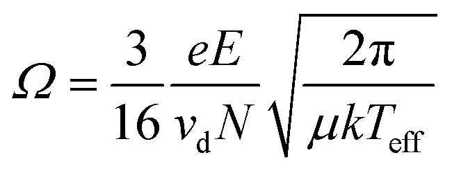 | (4) |
This discrepancy is not true, which prompted Siems et al. to correct the assumptions inherent in the Mason-Schamp equation as below:37
 | (5) |
 , and the correlation coefficients (ξ). These corrections are relatively simple and only require knowledge of parameters the experimentalist should already know or can easily calculate (i.e. velocity of the ion) and a detailed walk-through is included in the ESI.†37,38 However, the precise knowledge of experimental variables that enable these corrections is true only for primary principles mobility instruments (i.e. HiKE-IMS). Once mobilities can no longer be directly calculated, and a calibration step is required instead, then an additional source of error is introduced when not matching experimental conditions between platforms.
However, there is one condition for calculating CCS values that is routinely ignored but must be considered here and further corrected: clustering and dissociation. While efforts were taken here to mitigate clustering from water vapor as much as possible, some small amount of water vapor still enters the drift tube and clustering will happen. When an ion clusters with a water or other polar vapor molecule, the ion cluster changes mass and size compared to the protonated analyte ion which is routinely detected in a mass spectrometer. Additionally, depending on the experimental parameters (such as pressure and temperature) the time that an ion spends in a cluster changes, and therefore the actual mass of the ion/ion-cluster is functionally a weighted average based upon the cluster equilibrium.63 The only quantitative way to experimentally determine the equilibrium is by monitoring equilibrium shifts with changes in mobility by changing the concentration of the vapor modifier as ions decluster upon transfer to a mass spectrometer.64,65 Changing the temperature is another way to promote declustering. If it is assumed that the mobility changes as a function of reduced electric field (changing effective temperature) as obtained in alpha values only comes from declustering, then the alpha function can be used to establish a function for calculating the mass of the ion based on mobility changes. Ultimately, there is no way to determine the CCS of the protonated ion alone when clustering is present, and instead, CCS must be treated as a composite property of the ion-cluster and neutral.
Results
In Fig. 2, example spectra for all the halogenated anilines are shown, with all peaks labeled to clarify the discussion in the following sections. There are at least two peaks in every mobility spectrum labeled as peak 1 and peak 2. The third peak is present in nitrogen for some species labeled as peak 3. The origin and ionization of all three peaks have been examined in a previous publication for aniline and n-fluoroanilines and the other halogenated anilines display similar behavior with regard to the number of peaks.66 The reduced electric field in the reaction region was chosen because that is the value where peaks 1 and 2 have nearly the same intensities which allow for the characterization of both peaks as the reduced electric field in the drift region is changed. All ion mobilities, drift times, experimental parameters, CCS values, and alpha values for both peaks at all reduced electric field strengths are included in the ESI.† | ||
| Fig. 2 Spectra of every halogenated aniline in nitrogen at the same experimental conditions (ERR/N = 38 Td, EDR/N = 120 Td, all other parameters in Table 1). For all spectra, the 3 reactant ion peaks of NO+, O2+, and (H2O)nH3O+ are present at drift times between 0.3 and 0.35 ms. Under these conditions, aniline has its two peaks at drift times of 0.46 ms for peak 1 (molecular ion peak ionized via charge transfer or fragmentation) and 0.5 ms for peak 2 (protonated peak). In nitrogen, there are 3 peaks for multiple of the halogenated anilines, but since the extra peak is not present for all analytes, it is named peak 3 (protonated peak), despite eluting between peaks 1 and 2 for all anilines. All experimental details are in Table 1. | ||
In Fig. 3, the reduced mobilities of each halogenated aniline peak are shown as a function of reduced electric field strength in the drift region. Across all functional groups, similar trends in the mobilities relative to each substituent position are present. For peak 2, the highest mobility (smallest CCS) is ortho, followed by meta, followed by para for all tested halogenated anilines. For peak 1, the elution orders are different; ortho-substituted anilines still have the highest mobility (smallest CCS), then followed by para, and last meta. Since the only difference in each halogenated aniline series is the substituent position, the drive for changing mobility is likely due to either the shape of the molecule or changing the center of mass with substituent position. Sophisticated mobility modeling software would be needed to fully characterize differences due to substituent position.67 As previously reported for the fluoroanilines measured in N2,66 4-chloroaniline and 4-bromoaniline also have a third peak which elutes between the 3-substituted peak 1 and the 2-substituted peak 2. The change in mobility for peak 3 also appears parallel to the respective peak 1 which results in nearly the same alpha function. Again, these apparent parallel mobilities could be better examined with computational modeling which is outside the scope of this work.67
 | ||
| Fig. 3 The reduced mobilities for all peaks of chloroaniline, bromoaniline, and iodoaniline measured in nitrogen. All error bars are derived from one standard deviation of triplicate measurements of 500 signal averages. All experimental parameters are in Table 1. Large error bars at low E/N are caused by reduced ion transmission in the drift tube at these conditions lowering peak abundance. | ||
The last interesting thing to note about Fig. 3 is how the mobility of each aniline peak changes as a function of E/N as compared to their “low field” mobilities. This change in mobility as a function of E/N is plotted as the alpha values in Fig. 4, but to calculate alpha values, the mobility at “low field” needs to be defined. Due to the operating principles of the ion gate used in HiKE-IMS, the ion transmission through the ion gate, separating the reaction region from the drift region, depends on the ratio EDR/ERR of the electric fields in the reaction region and in the drift region: the lower this ratio, the lower the ion transmission. Thus, at low E/N in the drift region, while having high E/N in the reaction region, accurate peak fitting becomes difficult due to low peak intensity leading to larger errors regarding peak position and thus ion mobility. This error decreases as E/N in the drift region increases. However, for some analytes it is clear that there is no constant mobility at low electric field strength. For example, for peak 2 of 4-chloroaniline, the mobility constantly increases as a function of E/N. Other analytes have mobilities where they increase, then are constant for a small range of E/N, and then increase as expected by ion mobility theory, such as peak 2 of 2-iodoaniline. The behavior of each of these analytes as a function of E/N can be further explored with the alpha function in Fig. 4.
 | ||
| Fig. 4 For each of the para-substituted anilines, the alpha coefficients of both peaks are plotted in two different gases (air and N2) as a function of the E/N in the drift region. Alpha coefficients here are defined as in eqn (3a) where K0,E=0 is the average mobility of each peak at low E/N (>15 Td) as listed in Table 2. All experimental parameters listed in Table 1. | ||
In Fig. 4, the alpha function is graphed against reduced electric field strength for only the para-substituted anilines in N2 and in air. For clarity, the “low field” mobility values used to generate the alpha curves are listed in Table 2. The third aniline peak in nitrogen is omitted from this graph to allow a direct comparison between drift gas composition. The data for the meta-substituted and ortho-substituted are shown in Fig. S2 and S3.† Unsurprisingly, the α function changes in magnitude as a function of size. Stated differently, 4-fluoroaniline has the largest alpha value at high E/N (up to 0.7 for peak 2 in air) whereas 4-iodoaniline exhibits the smallest alpha value at high E/N (0.2 for peak 1 in N2). Similar to Fig. 3, some trends between the peaks are consistent across each halogen substitution. For both peaks in all analytes, measurements in air demonstrate a greater alpha value than those in nitrogen.
| Peak 1 | Peak 2 | |||||||
|---|---|---|---|---|---|---|---|---|
| Variable | K 0,E=0 (cm2 V−1 s−1) | α 2 (× 10−6) (V2 s2 cm−4) | α 4 (× 10−10) (V4 s4 cm−8) | R 2 | K 0,E=0 (cm2 V−1 s−1) | α 2 (× 10−6) (V2 s2 cm−4) | α 4 (× 10−10) (V4 s4 cm−8) | R 2 |
| 2-Fluoro | 1.914 | 8.3 ± 0.3 | −3.6 ± 0.3 | 0.884 | 1.744 | 5.3 ± 0.2 | −2.1 ± 0.1 | 0.940 |
| 3-Fluoro | 1.895 | 9.9 ± 0.3 | −4.5 ± 0.3 | 0.904 | 1.704 | 4.6 ± 0.1 | −1.7 ± 0.1 | 0.939 |
| 4-Fluoro | 1.90 | 8.4 ± 0.2 | −3.4 ± 0.2 | 0.941 | 1.70 | 5.9 ± 0.1 | −2.3 ± 0.1 | 0.946 |
| 2-Chloro | 1.834 | 6.7 ± 0.3 | −3.0 ± 0.3 | 0.752 | 1.695 | 3.5 ± 0.2 | −1.3 ± 0.2 | 0.838 |
| 3-Chloro | 1.799 | 7.5 ± 0.1 | −3.5 ± 0.1 | 0.215 | 1.626 | 3.8 ± 0.2 | −1.6 ± 0.1 | 0.098 |
| 4-Chloro | 1.806 | 7.8 ± 0.1 | −3.2 ± 0.1 | 0.975 | 1.602 | 5.1 ± 0.3 | −2.2 ± 0.3 | 0.997 |
| 2-Bromo | 1.769 | 5.7 ± 0.1 | −2.4 ± 0.1 | 0.931 | 1.638 | 4.7 ± 0.2 | −2.0 ± 0.2 | 0.775 |
| 3-Bromo | 1.728 | 6.2 ± 0.4 | −2.7 ± 0.3 | 0.652 | 1.564 | 2.7 ± 0.3 | −1.1 ± 0.3 | 0.358 |
| 4-Bromo | 1.738 | 4.8 ± 0.1 | −1.4 ± 0.1 | 0.956 | 1.539 | 3.1 ± 0.2 | −1.0 ± 0.2 | 0.845 |
| 2-Iodo | 1.713 | 5.0 ± 0.2 | −2.2 ± 0.2 | 0.792 | 1.588 | 3.1 ± 0.1 | −1.3 ± 0.1 | 0.825 |
| 3-Iodo | 1.667 | 5.8 ± 0.3 | −2.7 ± 0.3 | 0.519 | 1.507 | 3.4 ± 0.1 | −1.7 ± 0.1 | 0.707 |
| 4-Iodo | 1.68 | 3.9 ± 0.2 | −1.1 ± 0.2 | 0.789 | 1.48 | 2.9 ± 0.3 | −1.1 ± 0.3 | 0.360 |
Additionally, the shapes of the curves differ between each peak for all the anilines. Both peaks exhibit Type A behavior (semi-Gaussian shape), but only peak 1 of each aniline experiences a maximum value (or closely approaches it) for the drift region sweep performed. Peak 2 of all anilines is just a steady increase where only the smaller species show a decreased rate of increase and appear to approach their maximum. Peak 2 of the larger molecules (iodoaniline) have an alpha curve that looks almost exponential because the maximum value is at a higher E/N value than the HiKE-IMS is able to reach.
Finally, the alpha curves in Fig. 4 can be used to find alpha coefficients as defined in eqn (3b). The results are listed in Table 2 for all halogenated anilines. The trends between substitutions and halogen are consistent with what has already been discussed in Fig. 4. Namely, the change in mobility becomes less pronounced (α2 decreases) as the halogen gets larger. While these values may be useful to simulate how mobilities change as a function of E/N the last thing to note is the “goodness of the fit” for many of these species. For several of the anilines, the fit is less than ideal, especially for the meta-substituted anilines. Adding more alpha terms does not improve the fit either, because the deviation from the fit is largely due to the high degree of error in some of the measurements at low E/N due to low peak abundance caused by reduced ion transmission through the drift tube at low E/N. These fits do not diminish the capability of the alpha function to model changes in mobility as a function of reduced electric field strength. Therefore, the last ion mobility metric to discuss is converting into CCS values.
Fig. 5 displays both the traditional Mason-Schamp equation and the corrections made by Siems et al. for peak 2 of para-halogenated anilines with a few additional considerations.37,38 Where the corrections by Siems et al. are used,37,38 instead of using the mass of only the protonated ion (Fig. 5A), the ion is assumed to be an ion-hydronium cluster which declusters as EDR/N increases (Fig. 5B). To this purpose, a weighted average of the ion/ion-cluster mass scaled against the alpha functions in Fig. 4 under the assumption that the change in mobility only comes from declustering of the ion and can be used to estimate the reduced mass of the ion/ion-hydronium equilibrium. A more accurate treatment of the reduced mass as a function of clustering equilibrium would involve extensive computational modeling which is outside the scope of this manuscript. Additionally, for Mason-Schamp how the temperature term is handled is graphed in Fig. 5C (one temperature theory) and Fig. 5E (two-temperature theory). At “low fields” the CCS values for each species, however, at roughly 10 Td, the CCS values begin to change as a function of the electric field. This threshold for changing CCS values is higher in the uncorrected one-temperature Mason-Schamp equation (Fig. 5C) where the range of “nonstatic” CCS values can be extended up to roughly 20 Td depending on the analyte.
 | ||
| Fig. 5 For peak 2 of each of the para-substituted halogenated anilines, the ion-neutral collisional cross sections are plotted as a function of EDR/N as calculated by: Siems et al. (A), Siems et al. and weighting the ion mass as a function of alpha (B),37,38 Mason-Schamp equation (C), the difference between Mason-Schamp and Siems et al. (D), 2-temperature theory Mason-Schamp equation (E), and the difference between 2-temperature Theory and Siems et al. (F). If using Teff calculated from the reduced field strength with the Mason-Schamp equation, the difference in values compared to the corrections from Siems et al. is at most 5% with the highest error for larger ions.37,38 When neglecting Teff and using only the gas temperature, the difference between Mason-Schamp and the corrections from Siems et al. is up to 55%.37,38 | ||
Discussion
With the number of considerations made in Fig. 5, some nuance is needed to discuss the difference between the Mason-Schamp equation and the corrections from Siems et al.37,38 To cast the difference into more concrete terms, the percent difference between using the corrections of Siems et al.37,38 (both with a weighted mass to account for declustering, and assuming the mass of the ion is static) and the one (Fig. 5D) and two temperature (Fig. 5F) treatment of the Mason-Schamp equation are plotted. If using the reduced electric field strength to calculate and use the effective temperature, the difference of 5% change in CCS values is not egregious between the Mason-Schamp equation and Siems et al. in Fig. 5F.37,38 However, the two-temperature theory version of the Mason-Schamp equation is not the most common version used in secondary principle instruments operated at higher fields; the uncertainty of the field makes it impossible to calculate the effective temperature from the Wannier equation on these instruments, and the field uncertainty is the reason the mobility calibration procedures are used in the first place. Treating temperature as a static term results in CCS values that change less than all other calculation methods (Fig. 5C) which result in the largest difference in cross sections up to 55% for smaller more labile compounds (Fig. 5D). The last thing to note is there is little difference in the error whether the ion mass is treated as static or as a reduced average based on the alpha function. The first reason is that the weighting of the reduced mass is more heavily dependent on the neutral than the ion as ion mass increases. In this case, by adding a water molecule, the reduced mass changes by 1 Da at most. The second reason is due to the weighting of variables in the corrections by Siems et al.37,38 In these calculations (eqn (5)), the most emphasis is placed on the ratio of the velocity of the ion versus the thermal velocity of the neutral. These velocities are equal to each other (the definition of mid-field mobilities) between 100–115 Td depending on the ion; whereas the ratio of vt = 0.1vd that defines low-field mobilities is only present at less than 15 Td, with the exact value changing depending on the ion. Above this velocity ratio, the CCS values begin to change in both the Mason-Schamp equation and in the corrections by Siems et al.37,38However, another factor at play in driving the changes in mobility/CCS values may be the composition of the gas itself. In Fig. 4, the alpha curves between air and N2 often differ by a few %. This difference in alpha value between gases may indicate that the 21% O2 composition in air leads to a greater change in mobility as a function of electric field strength. O2 has a similar polarizability (1.564 Å3) to N2 (1.74 Å3),68 so it is possible, but unlikely, that polarizability of the neutral gas is the factor that causes a greater mobility change in air vs. N2 as a function of the electric field. The other explanation would stem from the ionization chemistry of HiKE-IMS where if more O2 is in the gas, there is more conversion to H3O+ ions and a greater probability of clustering.69,70 More experiments would need to be conducted in a variety of gases to explore if drift gas identity or polarizability plays a role in the degree of changing mobility as a function of EDR/N similar to effects previously reported in FAIMS systems.71
Whether or not the change in mobility stems only from clustering/declustering, there is still a significant change in ion mobilities and therefore cross sections as a function of reduced field strength. Without accounting for the change, errors in mobility and cross section can easily be propagated through calibration procedures for secondary mobility instruments such as TIMS and TWIMS if precautions are not taken. However, suitable calibrant mobility values at the field strengths needed for these instruments are mostly limited to atomic ions, which cannot be measured on these secondary instruments due to the low mass cut-off of the ion funnel traps used in these mobility devices. So how do we as IMS users, address this issue as a function of the electric field? First, there is an obvious, pressing need for a database of calibrant mobilities measured at high E/N on a primary principles mobility instrument (such as but not limited to HiKE-IMS). HiKE-IMS is uniquely well suited to this task as mobilities can be directly measured at varying field strengths and the low field mobilities for the anilines presented here are within experimental error for the same compounds measured on low field atmospheric pressure drift tube systems.66,72 However, current HiKE-IMS instruments are only suited for volatile compounds. These instrumental constraints make current HiKE-IMS instruments unable to investigate calibrants commonly used in “native” IM-MS, which requires an ion source capable of ionizing larger, nonvolatile compounds. Since there is a push that mobility calibrants need to match the same class as the desired analyte to ensure accuracy,73 a new HiKE-IMS coupled with electrospray ionization is under development to measure calibrants suited for “native” IM-MS.
Conclusion
While the work from Siems et al. is foundational and a valued discussion about what exactly is an ion-neutral collisional cross section, the implementation of their corrections has seen little use in the literature.37,38 Instead, most literature opts for the familiar Mason-Schamp equation or relies on calibration techniques built into commercial instrument software to obtain CCS values. Without careful consideration, errors due to incorrect assumptions based on the Mason-Schamp equation are not accounted for and greatly impact the calculation of CCS values. Siems et al. demonstrated the impact of these assumptions with data of atomic ions in atomic gases,38 but here, we provide the data of a series of halogenated anilines measured in two different drift gases on a first principle drift tube IMS (HiKE-IMS) across an order of magnitude in reduced electric field strength. By providing the data in metrics of reduced mobility, alpha functions, and the various ways to calculate CCS values, we not only show how mobilities change as a function of electric field strength, but how ignoring field strength magnifies error in CCS values. The error between CCS equations depends on the analyte and method of calculation, but in the most extreme case, the error in CCS value is over 50%.An error of over 50% in CCS value has multiple implications for measurement accuracy. When an error that high is inherent in the technique used to calculate CCS, how can an unknown analyte be identified with credulity based on CCS/mz alone? Additionally, modern mobility calibration techniques assume that CCS and mobilities are static from low-field calibrant mobilities into mid to high-field, which simply is not true for most analytes. This is an additional error that needs to be accounted for on top of corrections to the Mason-Schamp equation. Even if the IMS community as a whole switched to using K0 values instead of CCS values, K0 values also change as a function of reduced electric field strength. Regardless of the value used as an identifier, the need for calibrant mobilities at high field strengths are urgently needed.
In the ESI,† we are providing our mobilities of all halogenated anilines over all electric field strengths measured in both air and nitrogen. We recognize that aniline is not a universally ideal mobility calibrant, but by providing these mobilities, we hope they will be of use to the community either as calibrant mobilities obtained on a first-principles instrument or as a dataset to improve mobility modeling software. Regardless, more care needs to be taken when discussing ion mobility CCS values and the information that can be obtained from them.
It needs to be accounted that the used HiKE-IMS is only suited for volatile compounds, so that calibrants commonly used in “native” IM-MS cannot be investigated. This would require an ion source capable of ionizing larger, nonvolatile compounds. Therefore, a new HiKE-IMS coupled with electrospray ionization is under development to measure calibrants suited for “native” IM-MS.
Author contributions
Credit contributions: CNN: conceptualization, methodology, investigation, visualization, formal analysis. CS: visualization, methodology. SZ supervised the research project, and gave scientific and conceptual advice. All authors contributed to discussions and the manuscript.Conflicts of interest
The authors have no conflicts of interest to declare.Acknowledgements
Funded by the Deutsche Forschungsgemeinschaft (DFG, German Research Foundation) – 318063177 and 390583968.References
- H. Zaknoun, M.-J. Binette and M. Tam, Int. J. Ion Mobility Spectrom., 2019, 22, 1–10 CrossRef.
- L. M. Matz and H. H. Hill Jr., Anal. Chem., 2001, 73, 1664–1669 CrossRef CAS PubMed.
- J. R. Verkouteren and J. L. Staymates, Forensic Sci. Int., 2011, 206, 190–196 CrossRef CAS.
- J. R. Verkouteren, J. Lawrence, R. Michael Verkouteren and E. Sisco, Anal. Methods, 2019, 11, 6043–6052 RSC.
- A. McKenzie-Coe, J. D. DeBord, M. Ridgeway, M. Park, G. Eiceman and F. Fernandez-Lima, Analyst, 2015, 140, 5692–5699 RSC.
- R. G. Ewing, D. A. Atkinson, G. A. Eiceman and G. J. Ewing, Talanta, 2001, 54, 515–529 CrossRef CAS PubMed.
- M. A. Mäkinen, O. A. Anttalainen and M. E. T. Sillanpää, Anal. Chem., 2010, 82, 9594–9600 CrossRef.
- S. Pfammatter, E. Bonneil, F. P. McManus, S. Prasad, D. J. Bailey, M. Belford, J.-J. Dunyach and P. Thibault, Mol. Cell. Proteomics, 2018, 17, 2051–2067 CrossRef CAS.
- M. F. Bush, I. D. G. Campuzano and C. V. Robinson, Anal. Chem., 2012, 84, 7124–7130 CrossRef CAS PubMed.
- J. W. McCabe, C. S. Mallis, K. I. Kocurek, M. L. Poltash, M. Shirzadeh, M. J. Hebert, L. Fan, T. E. Walker, X. Zheng, T. Jiang, S. Dong, C.-W. Lin, A. Laganowsky and D. H. Russell, Anal. Chem., 2020, 92, 11155–11163 CrossRef CAS PubMed.
- M. T. Soper-Hopper, J. Vandegrift, E. S. Baker and F. M. Fernández, Analyst, 2020, 145, 5414–5418 RSC.
- G. Paglia, J. P. Williams, L. Menikarachchi, J. W. Thompson, R. Tyldesley-Worster, S. Halldórsson, O. Rolfsson, A. Moseley, D. Grant, J. Langridge, B. O. Palsson and G. Astarita, Anal. Chem., 2014, 86, 3985–3993 CrossRef CAS PubMed.
- C. M. Nichols, J. N. Dodds, B. S. Rose, J. A. Picache, C. B. Morris, S. G. Codreanu, J. C. May, S. D. Sherrod and J. A. McLean, Anal. Chem., 2018, 90, 14484–14492 CrossRef CAS PubMed.
- M. Schroeder, S. W. Meyer, H. M. Heyman, A. Barsch and L. W. Sumner, Metabolites, 2020, 10(1), 13 CrossRef CAS PubMed.
- B. S. Rose, J. C. May, A. R. Reardon and J. A. McLean, J. Am. Soc. Mass Spectrom., 2022, 33, 1229–1237 CrossRef CAS PubMed.
- K. L. Leaptrot, J. C. May, J. N. Dodds and J. A. McLean, Nat. Commun., 2019, 10, 985 CrossRef PubMed.
- K. M. Hines, J. C. May, J. A. McLean and L. Xu, Anal. Chem., 2016, 88, 7329–7336 CrossRef CAS PubMed.
- G. Paglia, M. Kliman, E. Claude, S. Geromanos and G. Astarita, Anal. Bioanal. Chem., 2015, 407, 4995–5007 CrossRef CAS.
- P. Benigni, J. Porter, M. E. Ridgeway, M. A. Park and F. Fernandez-Lima, Anal. Chem., 2018, 90, 2446–2450 CrossRef CAS PubMed.
- C. A. Olanrewaju, C. E. Ramirez and F. Fernandez-Lima, Energy Fuels, 2021, 35, 13722–13730 CrossRef CAS.
- G. Nagy, I. K. Attah, S. V. B. Garimella, K. Tang, Y. M. Ibrahim, E. S. Baker and R. D. Smith, Chem. Commun., 2018, 54, 11701–11704 RSC.
- P. Pathak, M. A. Baird and A. A. Shvartsburg, J. Am. Soc. Mass Spectrom., 2020, 31, 1603–1609 CrossRef CAS PubMed.
- J. N. Dodds, Z. R. Hopkins, D. R. U. Knappe and E. S. Baker, Anal. Chem., 2020, 92, 4427–4435 CrossRef CAS PubMed.
- J. N. Dodds, N. L. M. Alexander, K. I. Kirkwood, M. R. Foster, Z. R. Hopkins, D. R. U. Knappe and E. S. Baker, Anal. Chem., 2021, 93, 641–656 CrossRef CAS PubMed.
- E. S. Baker, K. E. Burnum-Johnson, J. M. Jacobs, D. L. Diamond, R. N. Brown, Y. M. Ibrahim, D. J. Orton, P. D. Piehowski, D. E. Purdy, R. J. Moore, W. F. Danielson 3rd, M. E. Monroe, K. L. Crowell, G. W. Slysz, M. A. Gritsenko, J. D. Sandoval, B. L. Lamarche, M. M. Matzke, B.-J. M. Webb-Robertson, B. C. Simons, B. J. McMahon, R. Bhattacharya, J. D. Perkins, R. L. Carithers Jr., S. Strom, S. G. Self, M. G. Katze, G. A. Anderson and R. D. Smith, Mol. Cell. Proteomics, 2014, 13, 1119–1127 CrossRef CAS PubMed.
- Y. M. Ibrahim, E. S. Baker, W. F. Danielson 3rd, R. V. Norheim, D. C. Prior, G. A. Anderson, M. E. Belov and R. D. Smith, Int. J. Mass Spectrom., 2015, 377, 655–662 CrossRef CAS PubMed.
- G. A. Eiceman, Z. Karpas and H. H. J. Hill, Ion Mobility Spectrometry, Taylor & Francis Group, Boca Raton, FL, 3rd edn, 2014 Search PubMed.
- J. A. Picache, B. S. Rose, A. Balinski, K. L. Leaptrot, S. D. Sherrod, J. C. May and J. A. McLean, Chem. Sci., 2019, 10, 983–993 RSC.
- M. E. Ridgeway, C. Bleiholder, M. Mann and M. A. Park, Trends Anal. Chem., 2019, 116, 324–331 CrossRef CAS.
- I. D. G. Campuzano and K. Giles, Trends Anal. Chem., 2019, 120, 115620 CrossRef CAS.
- J. R. N. Haler, C. Kune, P. Massonnet, C. Comby-Zerbino, J. Jordens, M. Honing, Y. Mengerink, J. Far and E. De Pauw, Anal. Chem., 2017, 89, 12076–12086 CrossRef CAS PubMed.
- C. N. Naylor, T. Reinecke, M. E. Ridgeway, M. A. Park and B. H. Clowers, J. Am. Soc. Mass Spectrom., 2019, 30, 2152–2162 CrossRef CAS PubMed.
- V. Gabelica and E. Marklund, Curr. Opin. Chem. Biol., 2018, 42, 51–59 CrossRef CAS PubMed.
- S. M. Stow, T. J. Causon, X. Zheng, R. T. Kurulugama, T. Mairinger, J. C. May, E. E. Rennie, E. S. Baker, R. D. Smith, J. A. McLean, S. Hann and J. C. Fjeldsted, Anal. Chem., 2017, 89, 9048–9055 CrossRef CAS PubMed.
- G. M. Thomson, J. H. Schummers, D. R. James, E. Graham, I. R. Gatland, M. R. Flannery and E. W. McDaniel, J. Chem. Phys., 1973, 58, 2402–2411 CrossRef CAS.
- E. V. Krylov, E. G. Nazarov and R. A. Miller, Int. J. Mass Spectrom., 2007, 266, 76–85 CrossRef CAS.
- W. F. Siems, L. A. Viehland and H. H. Hill Jr., Anal. Chem., 2012, 84, 9782–9791 CrossRef CAS PubMed.
- W. F. Siems, L. A. Viehland and H. H. Hill, Analyst, 2016, 141, 6396–6407 RSC.
- A. T. Kirk, M. Allers, P. Cochems, J. Langejuergen and S. Zimmermann, Analyst, 2013, 138, 5200–5207 RSC.
- A. T. Kirk, D. Grube, T. Kobelt, C. Wendt and S. Zimmermann, Anal. Chem., 2018, 90, 5603–5611 CrossRef CAS PubMed.
- G. E. Spangler and C. I. Collins, Anal. Chem., 1975, 47, 403–407 CrossRef CAS.
- H. E. Revercomb and E. A. Mason, Anal. Chem., 1975, 47(7), 970–983 CrossRef CAS.
- M. Tabrizchi, Talanta, 2004, 62, 65–70 CrossRef CAS PubMed.
- M. Tabrizchi and F. Rouholahnejad, Talanta, 2006, 69, 87–90 CrossRef CAS PubMed.
- J. C. May, C. B. Morris and J. A. McLean, Anal. Chem., 2017, 89, 1032–1044 CrossRef CAS PubMed.
- E. Krylov, E. G. Nazarov, R. A. Miller, B. Tadjikov and G. A. Eiceman, J. Phys. Chem. A, 2002, 106, 5437–5444 CrossRef CAS PubMed.
- G. Papadopoulos, A. Svendsen, O. V. Boyarkin and T. R. Rizzo, J. Am. Soc. Mass Spectrom., 2012, 23, 1173–1181 CrossRef CAS PubMed.
- S. W. C. Walker, A. Mark, B. Verbuyst, B. Bogdanov, J. L. Campbell and W. S. Hopkins, J. Phys. Chem. A, 2018, 122, 3858–3865 CrossRef CAS PubMed.
- D. K. Schweppe, S. Prasad, M. W. Belford, J. Navarrete-Perea, D. J. Bailey, R. Huguet, M. P. Jedrychowski, R. Rad, G. McAlister, S. E. Abbatiello, E. R. Woulters, V. Zabrouskov, J.-J. Dunyach, J. A. Paulo and S. P. Gygi, Anal. Chem., 2019, 91, 4010–4016 CrossRef CAS PubMed.
- A. S. Hebert, S. Prasad, M. W. Belford, D. J. Bailey, G. C. McAlister, S. E. Abbatiello, R. Huguet, E. R. Wouters, J.-J. Dunyach, D. R. Brademan, M. S. Westphall and J. J. Coon, Anal. Chem., 2018, 90, 9529–9537 CrossRef CAS PubMed.
- J. L. Kaszycki, A. P. Bowman and A. A. Shvartsburg, J. Am. Soc. Mass Spectrom., 2016, 27, 795–799 CrossRef CAS PubMed.
- E. A. Mason and E. W. McDaniel, Transport Properties of Ions in Gases, Wiley-VCH Verlag GmbH, Weinheim, Federal Republic of Germany, 1988 Search PubMed.
- L. A. Viehland, Gaseous Ion Mobility, Diffusion, and Reaction, Springer International Publishing, 2019, vol. 3 Search PubMed.
- B. C. Hauck, W. F. Siems, C. S. Harden, V. M. McHugh and H. H. Hill Jr., J. Phys. Chem. A, 2017, 121, 2274–2281 CrossRef CAS PubMed.
- B. C. Hauck, W. F. Siems, C. S. Harden, V. M. McHugh and H. H. Hill Jr., Rev. Sci. Instrum., 2016, 87, 075104 CrossRef PubMed.
- J. C. May, E. Jurneczko, S. M. Stow, I. Kratochvil, S. Kalkhof and J. A. McLean, Int. J. Mass Spectrom., 2018, 427, 79–90 CrossRef CAS PubMed.
- D. Hewitt, E. Marklund, D. J. Scott, C. V. Robinson and A. J. Borysik, J. Phys. Chem. B, 2014, 118, 8489–8495 CrossRef CAS PubMed.
- M. Landreh, C. Sahin, J. Gault, S. Sadeghi, C. L. Drum, P. Uzdavinys, D. Drew, T. M. Allison, M. T. Degiacomi and E. G. Marklund, Anal. Chem., 2020, 92, 12297–12303 CrossRef CAS PubMed.
- A. Kulesza, E. G. Marklund, L. MacAleese, F. Chirot and P. Dugourd, J. Phys. Chem. B, 2018, 122, 8317–8329 CrossRef CAS PubMed.
- D. Morsa, E. Hanozin, G. Eppe, L. Quinton, V. Gabelica and E. D. Pauw, Anal. Chem., 2020, 92, 4573–4582 CrossRef CAS PubMed.
- C. Bleiholder, F. C. Liu and M. Chai, Anal. Chem., 2020, 92, 16329–16333 CrossRef CAS PubMed.
- D. Morsa, E. Hanozin, V. Gabelica and E. De Pauw, Anal. Chem., 2020, 92, 16334–16337 CrossRef CAS PubMed.
- P. Kwantwi-Barima, H. Ouyang, C. J. Hogan Jr. and B. H. Clowers, Anal. Chem., 2017, 89, 12416–12424 CrossRef CAS PubMed.
- P. Kwantwi-Barima, C. J. Hogan Jr. and B. H. Clowers, J. Phys. Chem. A, 2019, 123, 2957–2965 CrossRef CAS PubMed.
- H. M. Schramm, T. Tamadate, C. J. Hogan and B. H. Clowers, Phys. Chem. Chem. Phys., 2023, 25(6), 4959–4968 RSC.
- C. N. Naylor, C. Schaefer, A. T. Kirk and S. Zimmermann, Phys. Chem. Chem. Phys., 2023, 25, 1139–1152 RSC.
- C. P. Harrilal, V. D. Gandhi, G. Nagy, X. Chen, M. G. Buchanan, R. Wojcik, C. R. Conant, M. T. Donor, Y. M. Ibrahim, S. V. B. Garimella, R. D. Smith and C. Larriba-Andaluz, Anal. Chem., 2021, 93, 14966–14975 CrossRef CAS PubMed.
- E. John and R. Rumble, CRC Handbook of Chemistry and Physics 99th Edition (Internet Version 2018), CRC Press/Taylor & Francis, Boca Raton, FL, 2018 Search PubMed.
- M. Allers, A. T. Kirk, M. Eckermann, C. Schaefer, D. Erdogdu, W. Wissdorf, T. Benter and S. Zimmermann, J. Am. Soc. Mass Spectrom., 2020, 31, 1291–1301 CrossRef CAS PubMed.
- M. Allers, A. T. Kirk, N. von Roßbitzky, D. Erdogdu, R. Hillen, W. Wissdorf, T. Benter and S. Zimmermann, J. Am. Soc. Mass Spectrom., 2020, 31, 812–821 CrossRef CAS PubMed.
- A. A. Shvartsburg, K. Tang and R. D. Smith, Anal. Chem., 2004, 76, 7366–7374 CrossRef CAS PubMed.
- H. Borsdorf, K. Neitsch, G. A. Eiceman and J. A. Stone, Talanta, 2009, 78, 1464–1475 CrossRef CAS PubMed.
- C. N. Naylor and B. H. Clowers, J. Am. Soc. Mass Spectrom., 2021, 32, 618–627 CrossRef CAS PubMed.
Footnote |
| † Electronic supplementary information (ESI) available. See DOI: https://doi.org/10.1039/d3an00493g |
| This journal is © The Royal Society of Chemistry 2023 |