
Dimensionality reduction for deep learning in infrared microscopy: a comparative computational survey†
Dajana
Müller
 ab,
David
Schuhmacher
ab,
Stephanie
Schörner
ac,
Frederik
Großerueschkamp
ac,
Iris
Tischoff
d,
Andrea
Tannapfel
ad,
Anke
Reinacher-Schick
ae,
Klaus
Gerwert
ac and
Axel
Mosig
*ab
ab,
David
Schuhmacher
ab,
Stephanie
Schörner
ac,
Frederik
Großerueschkamp
ac,
Iris
Tischoff
d,
Andrea
Tannapfel
ad,
Anke
Reinacher-Schick
ae,
Klaus
Gerwert
ac and
Axel
Mosig
*ab
aRuhr University Bochum, Center for Protein Diagnostics, Bochum, 44801, Germany. E-mail: axel.mosig@ruhr-uni-bochum.de
bRuhr University Bochum, Faculty of Biology and Biotechnology, Bioinformatics Group, 44801, Germany
cRuhr University Bochum, Faculty of Biology and Biotechnology, Department of Biophysics, 44801, Germany
dInstitute of Pathology, Ruhr-University Bochum, 44789 Bochum, Germany
eDepartment of Hematology, Oncology and Palliative Care, Ruhr-University Bochum, Bochum, Germany
First published on 7th September 2023
Abstract
While infrared microscopy provides molecular information at spatial resolution in a label-free manner, exploiting both spatial and molecular information for classifying the disease status of tissue samples constitutes a major challenge. One strategy to mitigate this problem is to embed high-dimensional pixel spectra in lower dimensions, aiming to preserve molecular information in a more compact manner, which reduces the amount of data and promises to make subsequent disease classification more accessible for machine learning procedures. In this study, we compare several dimensionality reduction approaches and their effect on identifying cancer in the context of a colon carcinoma study. We observe surprisingly small differences between convolutional neural networks trained on dimensionality reduced spectra compared to utilizing full spectra, indicating a clear tendency of the convolutional networks to focus on spatial rather than spectral information for classifying disease status.
1. Introduction
Combining infrared microscopy with machine learning has become an established approach in biomedical research. This approach yields high-dimensional infrared spectra at spatial resolution. Utilizing these complex data for disease classification and other biomedical applications is generally challenging. One approach to make classification more accessible is to computationally reduce the dimensionality of infrared spectra to few representative components. In this comparative study, we systematically investigate how different approaches towards reducing the dimensionality of infrared pixel spectra affect machine learning performance.Infrared microscopy is a well-established tool in biomedical research due to its label-free and non-destructive characteristics.1 Many studies have shown its analytical potential, particularly in cancer research using either Fourier transform infrared (FTIR) microscopy2,3 or, more recently, much faster quantum cascade laser (QCL) based infrared microscopy.4,5 In an infrared microscopic image, the absorbance spectra at each pixel position represent fingerprints of the biochemical composition. As has been demonstrated in numerous studies,3,6–8 the highly resolved molecular information can be utilised to precisely localize different tissue components,3 recognize tumor,5 or distinguish different tumor subtypes6,8 with high sensitivity and specificity.
From the perspective of data analysis, infrared spectra are high-dimensional, and reducing their dimensionality without losing relevant information is important for several reasons, in particular in the context of infrared microscopy. A first reason is of practical nature: infrared microscopic images often capture large areas of cell or tissue samples, resulting in large datasets that require significant resources in terms of storage and high-performance computing. Reducing the dimensionality clearly promises to reduce the computational resource footprint for infrared microscopy based diagnostic studies.
Besides such practical resource considerations, dimensionality reduction is also relevant from a more theoretical perspective. In cell or tissue samples, molecular absorptions result from a heterogeneous mixture of a large number of different molecules. The molecular absorptions are further understood to be intertwined with Mie scattering caused by infrared wavelength-sized particles such as nuclei.9,10 Consequently, it makes sense to consider discriminative spectral differences between tissue components as being due to integral phenotypic changes. Dimensionality reduction can potentially identify a small number of abstract phenotypes that may reflect molecular or cellular mechanisms involved in certain tissue components or certain stages of a disease. In this sense, dimensionality reduction could support the biological interpretation of infrared spectra.
Since the physical processes that model the composition of infrared spectra in tissue samples are highly non-linear,9 it is difficult to identify a dimensionality reduction method whose mathematical assumptions decompose tissue spectra into physically meaningful components. This difficulty motivates our comparative computational study in the present manuscript: we assess how different dimensionality reduction methods disentangle spectra into a limited number of components by measuring how the reduction affects subsequent classification. Since recent progress in computational pathology has been boosted significantly by deep convolutional neural networks, both for infrared imaging5,11,12 and conventional histopathology imagery,13 we focus on studying the effect of dimensionality reduction on such deep neural networks.
The remaining parts of the manuscript are structured as follows: we first provide a brief overview of dimensionality reduction approaches that are currently relevant for infrared microscopy. We then describe a QCL-based dataset of colon tissue samples used in a recent study5 in the context of tumor identification of colon carcinoma and describe in more detail five dimensionality reduction methods that we investigate. We then systematically compare how the five reduction approaches affect the performance of a specific weakly supervised deep learning method5 that localizes tumor. Our investigation aims to provide guidance for the use of dimensionality reduction in future studies, which we further support by making implementations available.
1.1. Dimensionality reduction approaches for infrared microscopy
Dimensionality reduction is commonly used in infrared microscopy for reducing computational resource demand and for disentangling biochemically relevant components of pixel spectra. Correspondingly, it has been discussed extensively in the context of preprocessing infrared pixel spectra.14 An elementary dimensionality reduction approach is to perform feature selection, i.e., to reduce the pixel spectra to only a few putatively relevant wavenumbers. In the early days of the field,15 handcrafted spectral features from wavenumbers selected based on prior knowledge. A major limiting factor for such knowledge-based approaches may be the complex composition of infrared microscopic pixel spectra, which has led to the investigation of data-centric approaches that infer relevant wavenumbers using statistical16 or information theoretic17 measures of significance to identify relevant wavenumbers.Whether based on prior knowledge or data-centric measures of significance, selecting individual wavenumbers for dimensionality reduction does not match the physical composition of wavenumbers. A more realistic, although still crudely oversimplified, assumption is to consider infrared spectra as linear combinations of base spectra associated with basic molecular or cellular constituents. This perspective leads straight to principal component analysis (PCA) and related factorization based dimensionality reduction approaches. Correspondingly, PCA has been utilized extensively in numerous studies.18–20 Also, methodologically related factorization approaches such as maximum noise fraction21 or vertex component analysis have been employed to reduce pixel spectra dimensionality. Such factorization approaches are indeed appealing for infrared spectroscopy since they make more explicit assumptions such as non-negativity of factors and noise characteristics.
It can be regarded as well-understood that the linearity assumptions underlying factorization based approaches do not match the involvement of non-linear processes9 in the composition of infrared spectra. This motivates the investigation of non-linear dimensionality reduction approaches such as local linear embedding,22,23 isomap24 and uniform manifold approximation and projection25 (UMAP). In ref. 26, UMAP was performed to reduce the dimensionality of spectral data in the context of neurodegenerative diseases classification. Autoencoders (AEs) constitute a neural network based class of dimensionality reduction approaches which have been investigated in the context of infrared spectroscopy based cancer classification27,28 as well as for noise reduction.29
2. Materials and methods
2.1. Sample preparation
Our study is based on a previously described cohort of 200 samples5 from the multicenter registry study ColoPredict Plus (CPP) 2.0 (registration number 4453-12, 20-6830 and 17-6151, Ethics Commission, Faculty of Medicine, Ruhr-University Bochum), which we briefly describe for the sake of completeness. The CPP 2.0 study collects samples retrospectively and prospectively in different clinical centers in Germany. The cohort includes 100 tumor-free tissue sections and 100 samples with colorectal carcinoma (UICC-Stage II and III, older than 18 years). Tissue samples were collected during surgery, formalin-fixated, followed by a paraffin-embedding, and handled according to standardized protocols used at the Institute of Pathology, Ruhr-Universität Bochum, Germany. Subsequently, the tissue blocks were cut into 7 μm thin tissue sections, placed onto Leica PET frame slides, and dewaxed before spectral data acquisition.2.2. Spectral data acquisition
Infrared imaging was performed using three Spero QT QCL-based microscopes which we refer to as Spero1–3 and the Chemical Vision software (Daylight Solutions, CA, USA) following an established setup (Kuepper et al., 2018).4 The standard microscope is equipped with a 4× magnification 0.3 NA objective, covering a 2 × 2 mm2 field of view (FOV). Spectra were obtained in the range of 1800 to 948 cm−1 with a spectral resolution of 2 cm−1 so that each pixel is represented by a 427-dimensional vector. Collection of chemical images is achieved with an uncooled focal plane array (FPA) detector, consisting of 480 × 480 pixels resulting in a pixel size of 4.25 × 4.25 μm for the given FOV. Following the spectral acquisition, the samples were stained by H&E according to the standard procedures in pathology.2.3. Datasets
The dataset of 200 samples was divided into a 50% training, 25% validation, and 25% testing ratio, with an equal distribution of tumor and tumor-free patients (Table 1). Training and validation sets were utilized in the training process while the test group was subsequently used for an independent evaluation. All groups were strictly separated at patient level, thus measurements of the same patient can only be found in one group. The partitioning of samples was kept constant throughout all experiments. For every sample, rectangular regions of interest (RoIs) of varying sizes were manually predefined to ensure a variety of tissue components in tumor-free samples and for tumor samples, at least 20% of cancerous tissue had to be present. Every RoI is labeled at patch-level, assigning each RoI as class label 1 if it contains tumor-related tissue and 0 otherwise. A binary mask for every RoI is available, in which tissue pixels are set to 1 and background pixels to 0.| Training cohort | Validation cohort | Test cohort | Total | ||||
|---|---|---|---|---|---|---|---|
| Tumor | Tumor-free | Tumor | Tumor-free | Tumor | Tumor-free | ||
| Samples (n) | 50 | 50 | 25 | 25 | 25 | 25 | 200 |
| Measurements (n) | 133 | 104 | 72 | 52 | 57 | 58 | 476 |
| Spero1 (n) | 100 | 53 | 58 | 27 | 46 | 28 | 312 |
| Spero2 (n) | 30 | 51 | 11 | 25 | 10 | 30 | 157 |
| Spero3 (n) | 3 | 0 | 3 | 0 | 1 | 0 | 7 |
| RoI (n) | 632 | 635 | 312 | 315 | 236 | 359 | 2489 |
| Subset | |||||||
| Samples (n) | 21 | 22 | 10 | 11 | 10 | 10 | 84 |
| Spectra (n) | 949![[thin space (1/6-em)]](https://www.rsc.org/images/entities/char_2009.gif) 183 183 |
736950 |
592188 |
346561 |
435349 |
468090 |
3528321 |
For all dimensionality reduction approaches, an additional subset of the whole dataset was used. The subset includes a randomized selection of samples from each group following the previous partitioning. It comprises 43 samples (21 tumor, 22 tumor-free) from the training data and 21 validation samples (10 tumor, 11 tumor-free). To further reduce the number of spectra, only 10% of spectra were randomly selected from each RoI. The training data involves a total of 1.68 million spectra and validation was conducted on 0.9 million spectra.
2.4. Dimensionality reduction
Each hyperspectral infrared image comprises infrared spectra where each pixel is represented as a spectrum with d = 427 wavenumbers. The dimensionality of the data was reduced to d = 16 to lower the computational complexity while retaining the most significant information in the data. The choice of reducing the dimensionality to 16 was determined by calculations of CompSegNet using encoded data of varying dimensions, specifically d = 4, 9 and 32 (ESI Table 1†). Reducing the dataset to 4 dimensions proved too limited, resulting in significant loss of information and poorer metric values. Conversely, reducing it to 32 dimensions did not provide substantial improvements compared to 9 dimensions (ESI Fig. 1†). Therefore, the selection of 16 dimensions strikes a balance between computational time and the risk of overfitting, ensuring the model's ability to generalize well to unseen data while keeping calculations within a day's time. For dimensionality reduction, we investigated five unsupervised methods, namely principal component analysis, uniform manifold approximation and projection, two different types of stacked autoencoders, and the selection of random wavenumbers as baseline (Fig. 1).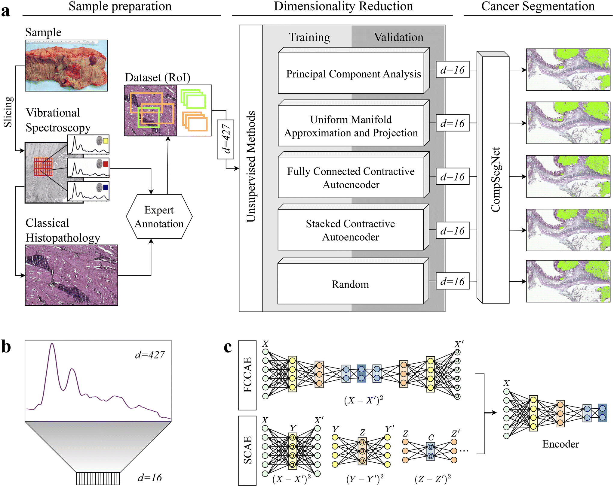 | ||
| Fig. 1 Schematic overview of the general workflow. a: Colon samples were measured with a quantum cascade laser and subsequently H&E stained. After getting expert annotations, regions of interest for control and cancer samples of varying sizes are defined. On only a subset, dimensionality reduction was performed with principal component analysis, uniform manifold approximation and projection, two autoencoders, and random projection in which random wavenumbers were chosen. To evaluate the encodings, a segmentation task was conducted using CompSegNet, yielding a cancer segmentation map. b: Each pixel in an infrared image is represented by a 427-dimensional vector and is embedded into a 16-dimensional space. c: Two contractive autoencoders were tested for dimensionality reduction: a series of stacked contractive autoencoder with a single hidden layer were trained36 and afterwards connected to form a deep autoencoder (SCAE, lower). In the second approach, all hidden layers were jointly trained, yielding a fully-connected contractive autoencoder (FCCAE, upper). | ||
In the optimization process, the local distances of the embedded data points to be preserved can be adjusted by a minimum distance parameter.25 For our UMAP approach, all combinations of a set of minimum distances min_dist = 0.01, 0.1, 0.5, 1, a set of k-neighbours for each data point n_neighbors = 5, 15, 50, 100 and eight metrics to compute the distance between points metric = {braycurtis, canberra, chebyshev, correlation, cosine, euclidean, manhattan, minkowski} were tested on a standardized test dataset, consisting of 100 healthy and 100 cancerous pixel spectra. The data was embedded into a Euclidean space (n_componetns = 2) for visualization. All metrics showed similar results under identical parameters. The default parameters for minimum distance and number of neighbors worked best for the majority of metrics, so for our dimensionality reduction study, we choose min_dist = 0.01, n_neighbors = 15, metric = correlation and a dimensional space of n_components = 16.
2.5. Cancer segmentation with CompSegNet
To evaluate the encoded datasets created by our dimensionality approaches, a cancer segmentation task was subsequently performed. A Comparative Segmentation Network (CompSegNet)5 was trained for each of the five dimensionality reduction methods. The network was trained on the full colon dataset described in section 2.3. The CompSegNet is a weakly supervised method using coarse-grained labels on patch-level only to overcome the bottleneck of requiring pixel-precise segmentations for localizing tumor or other relevant tissue components. The topology of CompSegNet comprises an extended U-Net39 architecture, whose input layer we adapted to the 16-dimensional input image features at each pixel. The output layer of the U-Net yields an activation map of equal spatial dimensions as the input data and is connected to a pooling neuron p. The activation of each neuron is bounded by a sigmoid function between 0 and 1 and is averaged in p, using the corresponding binary mask for each sample. The pooled activation is weighted by the relative amount of foreground pixels in each mask, giving a percentage of tumor present. The activation for control samples should be minimized while the activation for tumor samples should lie between a lower bound α and an upper bound α + β, to counteract overdetection of cancer.A total of 12 CompSegNet models for each approach were trained to allow for hyperparameter optimization and to find the combination of parameters yielding the highest metric values. Building on previous work,5 cancer patches were assumed to contain between 20% (α = 0.2) and 90% (α + β = 0.9) tumor, which was optimized among all combinations of α ∈ 0.05, 0.1 and α + β ∈ 0.8, 0.85, 0.9. We used a set of initial learning rates (5 × 10⁻⁴, 1 × 10⁻⁴) along with a learning rate scheduler (decay = 0.9 every 10 or 30 epochs) and a batch size of 4. RMSprop was the optimizer of choice with a momentum of 0. The models were trained for 400 epochs but were terminated earlier if overfitting occurred.
2.6. Model selection and binarization of activation maps
After training, each epoch is evaluated on validation data with a classification approach. The relative amount of activation in each RoI is calculated by taking the overall sum of activation and divide it by the sum of tissue pixels. If the resulting value lays between α and α + β, the RoI is labeled as 1 (cancer), 0 otherwise. The model yielding the highest F1 score of each approach is chosen.In the next step, activation maps have to be binarized to be comparable to groundtruth annotation. Therefore, we make use of two different thresholds θ and ρ, similar to Schuhmacher et al., 2022.5 The first threshold θ actually binarizes the image while the second threshold acts as a tumor-fraction threshold with an upper bound. The combination of both thresholds will classify a RoI as cancerous if the ratio of tumor pixels exceed ρ but is still below 90% of existing tissue pixels after binarization using θ. We systematically computed all possible combinations with a step size of 0.01 for θ and 0.02 for ρ to maximize F1 scores.
2.7. Implementation
All calculations were conducted on either of two different hardware constellations. First, a server (HPC) with an Intel(R) Xeon(R) Platinum 8176 CPU Processor with 56 CPU threads and 1.5 TB of RAM and an Nvidia Tesla V100 PCIe with 16 GB memory size; and second, a server (DL) an Intel(R) Xeon(R) Gold 6148 CPU Processor with 44 CPU threads with 385 GB of RAM with an Nvidia Tesla V100 SXM2 with 32 GB memory size. All computations on the HPC were implemented in Python (version 3.7.10), using the libraries sklearn (version 0.23.1), umap (version 0.5.1), tensorflow-gpu (version 2.1.0), and numpy (version 1.20.2). Computations on the DL server were computed using python (version 3.7.3), sklearn (version 0.23.1), tensorflow-gpu (version 2.2.0), and numpy (version 1.18.5).3. Results
3.1. Encoding comparison using t-SNE
Four of the five dimensionality reduction approaches require unsupervised pre-training, which was conducted on the subset comprising 1.77 million spectra. Computing principal components (PC) and the subsequent projection took less than 10 minutes (Table 2), while UMAP required 1.5 hours. Training of the fully connected AE took around 1.5 days, and training the stacked AE required more than seven days. No training was required in the Random approach, in which the dimensions of the dataset were reduced to 16 randomly selected wavenumbers. All encoding approaches were compared to a neural network using full spectra (Schuhmacher et al., 2022).5| t train dim. red. model on subset (h) | t load data (train/val) + encode data (h) | t train model (h) | Validation data | Testing data | |||||||
|---|---|---|---|---|---|---|---|---|---|---|---|
| Sens. (%) | Spec. (%) | Acc. (%) | F1 (%) | Sens. (%) | Spec. (%) | Acc. (%) | F1 (%) | ||||
| PCA | ∼0.1 | ∼5 | ∼24 | 96.12 | 97.78 | 96.00 | 96.90 | 91.34 | 97.21 | 94.92 | 93.39 |
| UMAP | ∼1.5 | ∼500 | ∼24 | 92.23 | 96.51 | 94.39 | 94.21 | 93.53 | 94.43 | 94.08 | 92.54 |
| FCCAE | ∼36 | ∼5 | ∼24 | 95.79 | 97.78 | 96.79 | 96.73 | 96.55 | 95.54 | 95.94 | 94.92 |
| SCAE | ∼180 | ∼5 | ∼24 | 93.85 | 99.05 | 96.47 | 96.35 | 93.10 | 98.61 | 96.45 | 95.36 |
| Random | — | ∼2 | ∼24 | 99.35 | 97.46 | 98.40 | 98.40 | 97.41 | 94.25 | 95.43 | 94.36 |
| Full spectra | — | ∼2 | ∼168 | 94.94 | 99.69 | 97.33 | 97.24 | 95.40 | 97.77 | 96.82 | 96.00 |
In order to visualize and compare the latent space representations and decompositions, the t-SNE algorithm was applied to one test sample to further reduce the dimensions to Euclidean space. The chosen sample comprises different tissue types, including areas of cancer (1, red), crypts (2, green), lymphocytes (3, blue), muscle (4, cyan), and connective tissue (5, purple). A background area not covered with tissue is labeled as class 0 (black) and was also included (Fig. 2a). For classes 1–5, an area of 100 × 100 pixels is defined as the representative of each tissue class, with the exception of lymphocytes (blue rectangle), due to the limited amount of lymphocytes in the tissue. If background pixels were present in other classes, they were masked and left out in further analysis. In the next step, the spectral cut-outs of each class were combined and their embeddings were calculated by our 5 proposed techniques. To compare if each dimensionality reduction approach captures local data structures while preserving the global ones as well, t-SNE (perplexity = 10, 30, ESI Fig. 2 and 3†) was conducted on low-dimensional data while we also examined the ability of t-SNE to separate the tissue classes given the full spectral range (Fig. 2b, top row). Here, we focus on t-SNE embeddings of SCAE and random projection in comparison to embeddings given the full spectral range. The embeddings of all tissue classes are illustrated in a combined scatter plot for each method. No clear separation of clusters can be found in the combined scatter plots regardless of different perplexity values (ESI Fig. 2 and 3†) although all methods were able to separate the background pixels from the other data points, except UMAP. The only embedding method that forms more compact clusters and allows for a more visual separation is the SCAE. Here, clusters overlap in more sparse areas while the dense pixel clouds are located towards the edges of the plot: the main pixels of the tumor class are located in the middle of the plot, the crypts and connective tissue are in the upper left and right corner, the background and lymphocytes are to the left and right of the main cancer pixels and the muscle class is below. While such trends may be due to distortions in the two dimensional t-SNE projections, they are consistently observed under varying perplexity values for t-SNE embeddings.
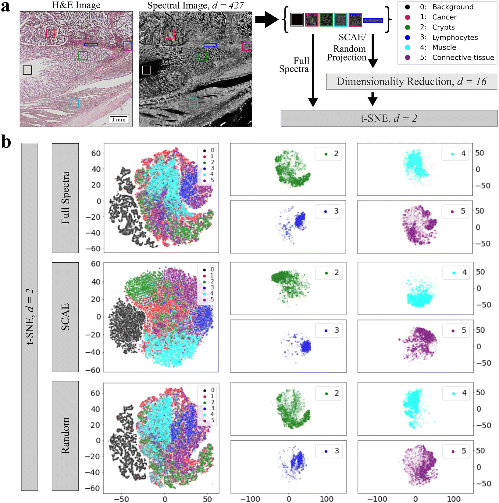 | ||
| Fig. 2 Comparison of encodings with t-SNE in Euclidean space. a: Spectral data of 6 different (tissue) classes (0, background, black; 1, cancer, red; 2, crypts, green; 3, lymphocytes, blue; 4, muscle, cyan; 5, connective tissue) from a test patient have been encoded with SCAE and random projection into 16 dimensions and were afterwards embedded into an Euclidean space with t-SNE. t-SNE was also conducted on full spectra for comparison. b: Results of t-SNE embeddings: each approach includes a main t-SNE plot showcasing the embeddings of all six classes. Additionally, a separate t-SNE plot is dedicated to classes 2, 3, 4, and 5, allowing a focused examination of these specific classes within the dataset. | ||
3.2. Computation time
As a next step, a cancer segmentation task is performed on the complete dataset. Therefore, a total of 1267 training and 627 validation data points (i.e., image patches) have to be embedded within each reduction approach. The loading time for full spectra takes approximately two hours (Table 2). Adding the embedding step, the overall loading and preprocessing time is extended by only 3 hours for PCA, FCCAE and SCAE. However, embedding with UMAP took around 3 weeks and the dataset was saved as an intermediate step. Reducing the wavenumbers of each dataset to 16 random numbers takes less than a second and can be neglected.Training the CompSegNet on full spectra for 400 epochs takes around one week, which is reduced to a training time of roughly one day on the dimensionality-reduced images. Thus, the overall training time could be decreased by 85%.
3.3. Deep learning classification performance
As described in section 2.6, the RoIs of the validation cohort that maximizes the F1 score were binarized, and a threshold on the number of tumor pixels classifies the sample as cancer or cancer-free, so that accuracy, sensitivity and specificity could be computed as performance measures. The results shown in Table 2 surprisingly indicate that classification on random wavenumbers yields sensitivity, accuracy and F1 score of 99.35%, 98.40% and 98.40%, respectively, exceeding the performance of any of the four non-trivial dimensionality reduction methods. The specificity score is one of the lowest (97.46%). The highest specificity of 99.69% was obtained using the full spectral range.For measuring performance on the independent test data, we used the same thresholds as for the validation data. The highest sensitivity score (97.41%) was likewise obtained by the random approach, while the highest specificity was obtained by the SCAE. The best accuracy and F1 scores were achieved by training on full spectra.
3.4. Cancer segmentation results
To evaluate cancer segmentations, the trained CompSegNet models were applied to a set of three whole-slide images from the test set using a sliding window of 256 × 256 with an offset of 64 pixels to obtain tumor segmentations. In overlapping areas of the sliding CompSegNet windows, the maximum activation was assigned to each pixel. Activation maps were binarized subsequently compared to groundtruth annotations taken from previous work.5 We used F1 scores to measure the performance of each cancer segmentation (Fig. 3, color: lime). Segmentations were further divided into true-positive pixels (yellow), false-positive areas (green) and false-negative ones (purple). The F1 scores of all five methods indicate a good agreement between annotation and tumor associated areas, where random projection yields the highest score exceeding 81%. Remarkably, no major differences can be noticed when comparing segmentations on any of the five dimensionality reduction methods to the segmentation obtained using full spectra. Only segmentations based on UMAP embeddings exhibit a significant amount of false positive pixels.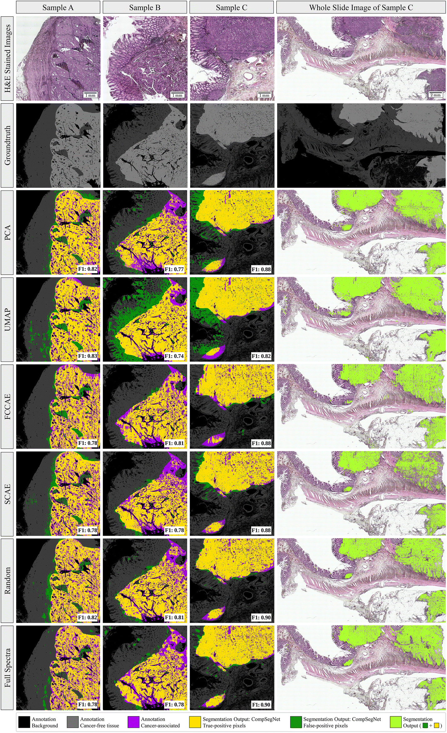 | ||
| Fig. 3 Comparison of whole-slide cancer segmentation on infrared samples and embeddings. Segmentations of 3 different samples of the independent test cohort of the ColoPredict Plus 2.0 registry study. Black: background of sample with no tissue. Grey: annotation of cancer-free tissue. Light grey: annotation of cancer tissue. Purple: cancer-associated tissue that is not detected by the neural network (false-negative). Yellow: segmentation output of cancerous pixels (true-positive). Green: segmentation output of hypothetical cancerous pixels (false-positive). Lime: segmentation output (green + yellow). Annotations were performed on H&E slides by a pathologist. | ||
In order to assess how far the classifiers rely on tissue morphology rather than spectral information, we created a morphology-free dataset by shuffling spectra randomly within each tile. As shown in ESI Fig. 4,† this results in a vanishing F1 score of the resulting segmentations on pixel level, while the classification of complete RoIs remains high (ESI Table 2†). This underlines the CompSegNet's heavy reliance on tissue morphology for accurate segmentations.
4. Discussion
The most striking and remarkable phenomenon we observe are the relatively small differences in performance, not only between the five dimensionality reduction methods, but also compared to training on full spectra. This indicates that, at least in the tumor localization task under our investigation, the convolutional neural network makes only limited use of spectral information for classification, which is underlined by the vanishing F1 score in a pixel permuted dataset. This is further supported by the unexpectedly strong performance of random projection. The neural networks not exploiting spectral information clearly suggests that classifications of infrared microscopic images by convolutional neural networks can utilize morphological or other spatial information. Two aspects remain open: first, it is unclear what is the physical origin of the spatial information, which could be due to morphological patterns of molecular vibrations, or result from (resonant) Mie scattering of cells or subcellular particles.40 While it is interesting that spatial information contained in infrared microscopic images is useful for classifying disease status, it is also dissatisfying. It suggests that the strong improvements in terms of accuracy and model generalization seen in recent infrared-microscopy based tissue diagnostic studies5,41 are at least partially due to spatial information. This clearly calls for the exploration of machine learning models that systematically exploit spectral information, while matching or exceeding the steep improvements in accuracy and model generalization that convolutional neural networks brought to the field recently.While differences between the four non-trivial embedding methods under investigation are small, they are far from negligible. The computationally very efficient PCA appears to be competitive with the much more resource demanding methods, which yet must be taken with a grain of salt. Only one out of the twelve CompSegNet models trained on PCA embedded spectra yielded reasonable segmentations, while the embeddings by the UMAP, FCCAE, SCAE and also random projection were much less sensitive to CompSegNet parameter settings. The t-SNE projections in Fig. 2 indicate that the SCAE conserves both local and global spectral information more strongly than any of the other methods. UMAP somewhat falls behind, not only because of high computation times, but also false positive tumor identification.
Dimensionality reduction clearly delivers the promise of resource efficient training of strong disease classifiers by reducing the time needed for training by almost one order of magnitude, while achieving essentially identical performance compared to using full spectra. This finding, however, cannot be transferred to arbitrary settings: our results do not exclude that in other settings, e.g. when dealing with classifying or localizing cancer subtypes,8,42,43 performance could suffer significantly under dimensionality reduction. The same holds for neural network topologies other than the CompSegNet investigated here, which could potentially be more or less sensitive to dimensionality reduction.
5. Conclusions
We have systematically compared how five different dimensionality reduction approaches applied to infrared microscopic pixel spectra affect subsequent disease classification by convolutional neural networks. Our most striking finding is that convolutional neural networks, at least in the setting given here, make strong use of spatial information rather than spectral information for disease classification, raising the quest for future developments of machine learning approaches that incorporate both levels of information. Yet, dimensionality reduction significantly reduces the resource demand required to train stable machine learning models, suggesting that low dimensional embeddings are a useful tool for establishing infrared microscopy based tissue diagnostics, at least in classification tasks where spatial context is informative for classification.Code and data availability
The source code to perform dimensionality reductions is available at https://github.com/RUB-Bioinf/DimensionalityReduction. A suitable docker image can be downloaded here: https://hub.docker.com/r/bioinfbo/dimensionality_reduction. The spectral and medical data that support the findings of this study are available from the corresponding author AM upon reasonable request.Author contributions
Conceptualization: DM, AM; data curation: SS, FG; formal analysis: DM; funding acquisition: KG, AM, AT, ARS; investigation: DM, AM; methodology: DM, AM, DS; project administration: KG, FG, AM; resources: KG, AM, IT; software: DM; supervision: AM; validation: DM, AM; visualization: DM; writing – original draft: DM, AM; writing – review & editing: DM, AM, FG, SS, KG, AT, ARS.Conflicts of interest
The authors declare that they have no known competing financial interests or personal relationships that could have appeared to influence the work reported in this paper.Acknowledgements
The Center for Protein Diagnostics (PRODI) is funded by the Ministry of Culture and Science (MKW) of the State of North-Rhine Westphalia, Germany (grant number: 111.08.03.05-133974). Part of this research was conducted within the Slide2Mol project funded by the Computational Life Sciences program of the German Federal Ministry of Education and Research, grant number 031L0264.References
- E. Goormaghtigh, Biomed. Spectrosc. Imaging, 2016, 5, 325–346 Search PubMed.
- H. J. Byrne, M. Baranska, G. J. Puppels, N. Stone, B. Wood, K. M. Gough, P. Lasch, P. Heraud, J. Sulé-Suso and G. D. Sockalingum, Analyst, 2015, 140, 2066–2073 RSC.
- A. Kallenbach-Thieltges, F. Großerüschkamp, A. Mosig, M. Diem, A. Tannapfel and K. Gerwert, J. Biophotonics, 2013, 6, 88–100 CrossRef.
- C. Kuepper, A. Kallenbach-Thieltges, H. Juette, A. Tannapfel, F. Großerueschkamp and K. Gerwert, Sci. Rep., 2018, 8, 7717 CrossRef PubMed.
- D. Schuhmacher, S. Schörner, C. Küpper, F. Großerueschkamp, C. Sternemann, C. Lugnier, A.-L. Kraeft, H. Jütte, A. Tannapfel and A. Reinacher-Schick, et al. , Med. Image Anal., 2022, 82, 102594 CrossRef PubMed.
- A. Akalin, X. Mu, M. A. Kon, A. Ergin, S. H. Remiszewski, C. M. Thompson, D. J. Raz and M. Diem, Lab. Invest., 2015, 95, 406–421 CrossRef PubMed.
- C. Kuepper, F. Großerueschkamp, A. Kallenbach-Thieltges, A. Mosig, A. Tannapfel and K. Gerwert, Faraday Discuss., 2016, 187, 105–118 RSC.
- K. Gerwert, S. Schörner, F. Großerüschkamp, A.-L. Kraeft, D. Schuhmacher, C. Sternemann, I. S. Feder, S. Wisser, C. Lugnier, D. Arnold, et al..
- P. Bassan, A. Kohler, H. Martens, J. Lee, H. J. Byrne, P. Dumas, E. Gazi, M. Brown, N. Clarke and P. Gardner, Analyst, 2010, 135, 268–277 RSC.
- M. A. Brandsrud, R. Blümel, J. H. Solheim and A. Kohler, Sci. Rep., 2021, 11, 1–14 CrossRef PubMed.
- A. P. Raulf, J. Butke, C. Küpper, F. Großerueschkamp, K. Gerwert and A. Mosig, Bioinformatics, 2020, 36, 287–294 CrossRef CAS PubMed.
- P. Pradhan, S. Guo, O. Ryabchykov, J. Popp and T. W. Bocklitz, J. Biophotonics, 2020, 13, e201960186 CrossRef PubMed.
- J. Van der Laak, G. Litjens and F. Ciompi, Nat. Med., 2021, 27, 775–784 CrossRef CAS PubMed.
- P. Lasch, Chemom. Intell. Lab. Syst., 2012, 117, 100–114 CrossRef CAS.
- D. C. Fernandez, R. Bhargava, S. M. Hewitt and I. W. Levin, Nat. Biotechnol., 2005, 23, 469–474 CrossRef CAS PubMed.
- S. Banerjee, M. Pal, J. Chakrabarty, C. Petibois, R. R. Paul, A. Giri and J. Chatterjee, Anal. Bioanal. Chem., 2015, 407, 7935–7943 CrossRef CAS PubMed.
- S. D. Krauß, R. Roy, H. K. Yosef, T. Lechtonen, S. F. El-Mashtoly, K. Gerwert and A. Mosig, J. Biophotonics, 2018, 11, e201800022 CrossRef PubMed.
- I. V. Kovalenko, G. R. Rippke and C. R. Hurburgh, J. Near Infrared Spectrosc., 2007, 15, 21–28 CrossRef CAS.
- E. Kaznowska, J. Depciuch, K. Szmuc and J. Cebulski, J. Pharm. Biomed. Anal., 2017, 134, 259–268 CrossRef CAS PubMed.
- E. Kaznowska, J. Depciuch, K. Łach, M. Kołodziej, A. Koziorowska, J. Vongsvivut, I. Zawlik, M. Cholewa and J. Cebulski, Talanta, 2018, 186, 337–345 CrossRef CAS PubMed.
- R. K. Reddy and R. Bhargava, Analyst, 2010, 135, 2818–2825 RSC.
- S. T. Roweis and L. K. Saul, Science, 2000, 290, 2323–2326 CrossRef CAS PubMed.
- N. Qi, Z. Zhang, Y. Xiang and P. d. B. Harrington, Anal. Chim. Acta, 2012, 724, 12–19 CrossRef CAS PubMed.
- J. B. Tenenbaum, V. d. Silva and J. C. Langford, Science, 2000, 290, 2319–2323 CrossRef CAS PubMed.
- L. McInnes, J. Healy and J. Melville, arXiv preprint arXiv:1802.03426, 2018.
- L. Lovergne, D. Ghosh, R. Schuck, A. A. Polyzos, A. D. Chen, M. C. Martin, E. S. Barnard, J. B. Brown and C. T. McMurray, Sci. Rep., 2021, 11, 1–19 CrossRef PubMed.
- M. A. Aslam, C. Xue, Y. Chen, A. Zhang, M. Liu, K. Wang and D. Cui, Sci. Rep., 2021, 11, 1–12 CrossRef PubMed.
- C. He, S. Zhu, X. Wu, J. Zhou, Y. Chen, X. Qian and J. Ye, ACS Omega, 2022, 7, 10458–10468 CrossRef CAS PubMed.
- C. Zhang, L. Zhou, Y. Zhao, S. Zhu, F. Liu and Y. He, Chemom. Intell. Lab. Syst., 2020, 203, 104063 CrossRef CAS.
- J. A. Lee and M. Verleysen, Nonlinear dimensionality reduction, Springer, 2007, vol. 1 Search PubMed.
- R. Gautam, S. Vanga, F. Ariese and S. Umapathy, EPJ Tech. Instrum., 2015, 2, 1–38 CrossRef PubMed.
- I. T. Jolliffe and J. Cadima, Philos. Trans. R. Soc., A, 2016, 374, 20150202 CrossRef PubMed.
- E. Becht, L. McInnes, J. Healy, C.-A. Dutertre, I. W. Kwok, L. G. Ng, F. Ginhoux and E. W. Newell, Nat. Biotechnol., 2019, 37, 38–44 CrossRef CAS PubMed.
- M. W. Dorrity, L. M. Saunders, C. Queitsch, S. Fields and C. Trapnell, Nat. Commun., 2020, 11, 1–6 CrossRef PubMed.
- I. Goodfellow, Y. Bengio and A. Courville, Deep Learning, MIT Press, 2016 Search PubMed.
- S. Rifai, G. Mesnil, P. Vincent, X. Muller, Y. Bengio, Y. Dauphin and X. Glorot, Joint European conference on machine learning and knowledge discovery in databases, 2011, pp. 645–660.
- X. Glorot and Y. Bengio, Proceedings of the thirteenth international conference on artificial intelligence and statistics, 2010, pp. 249–256.
- L. Van der Maaten and G. Hinton, J. Mach. Learn. Res., 2008, 9, 2579–2605 Search PubMed.
- O. Ronneberger, P. Fischer and T. Brox, International Conference on Medical image computing and computer-assisted intervention, 2015, pp. 234–241.
- E. A. Magnussen, B. Zimmermann, U. Blazhko, S. Dzurendova, B. Dupuy-Galet, D. Byrtusova, F. Muthreich, V. Tafintseva, K. H. Liland and K. Tøndel, et al. , Commun. Chem., 2022, 5, 1–10 CrossRef PubMed.
- K. Gerwert, S. Schörner, F. Großerüschkamp, A.-L. Kraeft, D. Schuhmacher, C. Sternemann, I. S. Feder, S. Wisser, C. Lugnier and D. Arnold, et al. , Eur. J. Cancer, 2023, 122–131 CrossRef CAS PubMed.
- F. Großerueschkamp, A. Kallenbach-Thieltges, T. Behrens, T. Brüning, M. Altmayer, G. Stamatis, D. Theegarten and K. Gerwert, Analyst, 2015, 140, 2114–2120 RSC.
- N. Goertzen, R. Pappesch, J. Fassunke, T. Brüning, Y.-D. Ko, J. Schmidt, F. Großerueschkamp, R. Buettner and K. Gerwert, Am. J. Pathol., 2021, 191, 1269–1280 CrossRef CAS PubMed.
Footnote |
| † Electronic supplementary information (ESI) available. See DOI: https://doi.org/10.1039/d3an00166k |
| This journal is © The Royal Society of Chemistry 2023 |