
 Open Access Article
 This Open Access Article is licensed under a Creative Commons Attribution-Non Commercial 3.0 Unported Licence
Colloidal membranes of chiral rod-like particles
Anja
Kuhnhold
 *,
Nils
Göth
and
Nadja
Helmer
*,
Nils
Göth
and
Nadja
Helmer
Institute of Physics, University of Freiburg, 79104 Freiburg (Breisgau), Germany. E-mail: anja.kuhnhold@physik.uni-freiburg.de
First published on 27th December 2021
Abstract
We study colloidal (or smectic) membranes composed of chiral rod-like particles through Monte Carlo simulations. These objects are formed due to the presence of Asakura-Oosawa spheres acting as depletants and creating an effective attraction between the rods. The membranes' shape and structure can be influenced by several parameters, e.g. the number of spheres and rods, their length and their interaction. In order to compare simulation results to an elastic theory, we follow two ansatzes, approximating the free elastic energy in different ways. Both of them lead to reasonable results and capture the behaviour of the colloidal membrane system. One approximation, however, is not suited for achiral rods, where twisting occurs due to surface energy rather than elastic energy. We extract the inverse cholesteric pitch and twist penetration depth for chiral rods with this approximation. The other one is used to introduce a complementary method to estimate elastic constants from the shape of colloidal membranes. Besides, we describe the transition from homogeneously twisted membranes to membranes composed of substructures that occur when the chiral interaction exceeds a length-dependent threshold. We believe that our detailed study and discussion of different aspects of this model system are valuable from a fundamental research viewpoint and suitable for material design suggestions.
1 Introduction
Anisotropic particles are the basis of phases of matter beyond isotropic or crystalline: the orientational degrees of freedom allow for intermediate liquid-crystalline phases with different levels of symmetry. Such liquid crystals (LCs) have been subject to research for more than a century,1 and sustained studies of LC systems led to applications like liquid crystalline displays (LCDs) or optical sensors and usage in cosmetics and fashion.2 Even simple hard rod models that can be treated theoretically via standard approximations or computer simulations show a rich phase behaviour. On the experimental side, pertinent counterparts of such hard rod models are viruses.3,4 They are monodisperse by nature, and it is possible to tune their spatial dimensions and their interparticle interaction potential (e.g. by inducing mutations and coating the viruses with specific proteins). A speciality of the pair interaction between viruses is that it is chiral, which leads to a chiral nematic (or cholesteric) LC phase, where the orientation of the viruses (or the mesogens in general) rotates in space. However, not only the bulk phases are of interest; the present work was inspired by the various objects that arise from mixtures of viruses and polymers or colloids: tactoids (nematic droplets), 2d membranes, 1d ribbons and hexagonal crystalline platelets, to name a few.5–7 The polymers/colloids act as depleting agents and drive the assembly of the viruses into such finite objects. We encourage the reader to have a look into ref. 5, where one gets an excellent impression of these objects. The possibility to tune the hierarchical self-assembly of this system on several levels (individual viruses, pair interaction, collective behaviour) makes it a perfect model for research of new functional materials.The experimental findings are complemented by theoretical models and simulations that combine the insights and enhance this model's value. With our paper, we will add a further piece to that by performing and analysing extensive Monte Carlo simulations and by comparing the results to theoretical predictions. As a target object, we chose a colloidal membrane, i.e. a one-layer thick assembly of rods with a finite size and an almost circular shape. An example snapshot of a colloidal membrane is shown in Fig. 1. The rods do, in general, not point in the same direction but show some twist towards the edge to minimise the system free energy (details are discussed below). From a theoretical point of view, there are, for example, studies regarding the equation of state of colloidal membranes,9,10 the effective interaction between two of those membranes,11 and their coalescence.12,13 Further examples are the line tension of the membrane edge,14 the phase separation and raft formation in membranes composed of two species,15–21 and the twist angle profile that minimises the free energy.14,22 The latter will be discussed here as one of the main points. In other studies with a similar simulation model but a different research focus, colloidal membranes often span the simulation box in two dimensions and rods have constraints on the orientational degrees of freedom.23,24 Here, we explicitly include the membrane's boundary in our particle-based simulations and allow for arbitrary rod orientations.
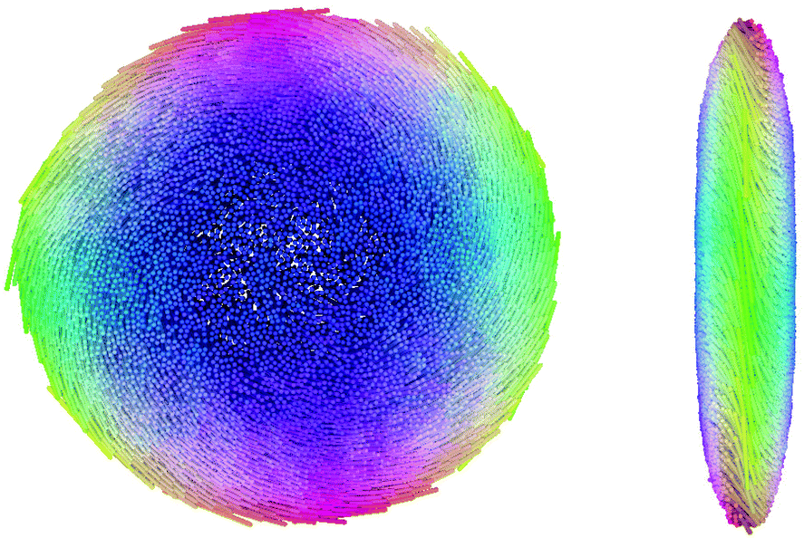 | ||
Fig. 1 Top (left) and side (right) view of a simulated colloidal membrane. The snapshot was rendered using POV-Ray8 and the colour codes the orientation of the rod-like particles. System parameters are N = 4900, ![[small script l]](https://www.rsc.org/images/entities/char_e146.gif) = 20, ε = 15 kBT. = 20, ε = 15 kBT. | ||
Approximations of the free energy of liquid crystalline systems are usually based on a continuum description using the Frank elastic energy. This includes different types of deformations of the nematic director field, which describes the LC mesogens' local orientation. Typically, one considers splay, twist and bend deformations that contribute to the elastic energy with weights given by the respective Frank elastic constant. However, details of the approaches vary from one-constant approximation to microscopic derivation of elastic constants, and there are also differences in the inclusion or neglect of further terms. We will use two versions of an approximation of the free energy: (1) using microscopic expressions for elastic constants and an effective 2d description (with fixed membrane radius), based on ref. 22. (2) A 3d description (with fixed membrane volume) similar to that introduced for tactoids (nematic droplets) in ref. 25, and parametric elastic constants. We do not judge which one is better, as this depends on the question at hand. However, we show how they can be applied to the colloidal membrane systems and offer a guide for studies on similar systems, including experimental ones.
A homogeneously twisted membrane can also be regarded as a single layer of a so-called double-twist cylinder.26 Double twist refers to having two axes around which the local orientation of particles (the director) rotates, in contrast to a single axis in a perfect cholesteric (or chiral nematic) phase. In a bulk system, double-twist cylinders (DTCs) cannot fill space so that defects arise naturally. The corresponding bulk phase is called blue phase, and there are several distinctions that depend on the arrangement of the DTCs. Recently, two-dimensional blue phases were found in experiment27 and simulation.28 In this phase, the DTCs are arranged in a hexagonal lattice, and the director in each DTC twists by π/2 from the centre to the edge (half-skyrmion structure). Continuum simulation also showed that the 2d blue phase could be preserved in confinement.28 We utilise particle-based simulations of a model chiral liquid crystal that lead to similar structures and complement the previous insights.
The paper is structured as follows. First, we explain the model and the simulations that we employ in Section 2. Then in Section 3, we discuss two versions of an approximate theory of the system's free energy. Afterwards, we describe and examine the simulation results, Section 4.1. We compare the simulation results to the first version of the theory in Section 4.2. The different terms that contribute to the free energy approximated by the second version are discussed in Section 4.3. In Section 4.4, we demonstrate how to estimate elastic constants from a comparison between simulation and theoretical results. In the last part, Section 4.5, we present the transition from homogeneous to substructured membranes. Finally, the conclusion is provided in Section 5.
2 Model and simulations
We employ particle-based Monte Carlo simulations to study the properties of colloidal membranes. The rod-like particles are modelled as spherocylinders with diameter D and length L. These rods are not allowed to overlap (hard-core repulsion) and have a distance- and orientation-dependent pair interaction based on Goossens' potential:29 | (1) |
![[m with combining circumflex]](https://www.rsc.org/images/entities/i_char_006d_0302.gif) i is the unit vector along the long axis of particle i and
i is the unit vector along the long axis of particle i and ![[r with combining right harpoon above (vector)]](https://www.rsc.org/images/entities/i_char_0072_20d1.gif) ij = rij
ij = rij![[r with combining circumflex]](https://www.rsc.org/images/entities/i_char_0072_0302.gif) ij is the distance vector between the particles' centres of mass. With this, the preferred angle between two rods is π/4. This model has already been studied concerning its bulk properties. It forms a cholesteric phase, with the inverse pitch being proportional to the chiral strength.30
ij is the distance vector between the particles' centres of mass. With this, the preferred angle between two rods is π/4. This model has already been studied concerning its bulk properties. It forms a cholesteric phase, with the inverse pitch being proportional to the chiral strength.30
Additionally, we add spherical particles that act as depletants to the rods and keep them assembled. They are modelled as Asakura-Oosawa spheres, i.e. they do not interact with each other, but they have a hard core repulsion with the rods (no overlap allowed). The sphere diameter was chosen to be twice that of the rods so that the number of spheres necessary to confine the rods is small enough to limit the computational cost but large enough to allow treating them as a pressure bath.
We apply Metropolis Monte Carlo (MC) simulations using an implicit depletants scheme for placing the spheres,31 that results in an NμDVT ensemble, with the number of rods N, the simulation box volume V, the temperature T, and the chemical potential of the depletants μD. In short, this means the spheres are no actual objects that are saved during the run, but they are put randomly around the rods for each rod move. If there is an overlap between the put sphere and the rod that was moved, and at the same time, there is no overlap between the sphere and the rod in its old position or any neighbouring rod, the move of the rod is rejected. If none of the spheres overlaps only with the rod that was moved, the Metropolis acceptance criterion is used to decide about accepting or rejecting the move finally: if the potential energy difference of the system in the new and old state ΔU = Unew − Uold < 0 the move is accepted, otherwise it will be rejected with a probability of 1 − exp(−ΔU/kBT). Here, kB is the Boltzmann constant, T is the absolute temperature, and kBT is used as the unit of energy. If the rods are achiral (ε = 0 kBT), only rod-rod and rod-sphere overlaps are checked. In practice, instead of their chemical potential μD, the depletants are characterised by their average number density ρD. The simulation box does have a fixed volume and periodic boundary conditions; however, due to the implicit depletants, the actual volume does not play a role as long as it is large enough to have the membrane not interacting with itself through any boundary.
In the initial setup, all rods point in the same direction, say z, their centres are fixed to a plane, which here corresponds to z = 0, and they are arranged in circular layers or on a hexagonal lattice. Then they are relaxed to adopt their equilibrium state. To achieve this, we randomly apply single-particle moves: translations within the chosen plane and rotations around arbitrary axes. During the equilibration, the maximum displacement and angle of rotation are adjusted to have an acceptance rate of 0.5. The equilibration takes at least several 105 MC sweeps (in one sweep, each rod has been tried to be moved once on average), but this strongly depends on the parameters and number of rods. A system is equilibrated when averaged quantities like nematic order parameter, system energy, membrane radius, and twist angle profile do not change anymore, apart from small fluctuations. Configurations of relaxed systems are also used as a starting point for simulations with other sets of parameters.
3 Theory
To study the behaviour of liquid crystalline systems from a theoretical point of view, one commonly tries to compute the systems' free energy. For these systems, the main contributions to the free energy originate from deformations of the director field. These contributions can be described by the Frank elastic energy, which for a bulk chiral nematic phase is:32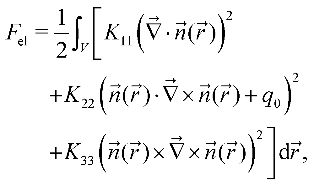 | (2) |
![[n with combining right harpoon above (vector)]](https://www.rsc.org/images/entities/i_char_006e_20d1.gif) () is the nematic director field, and q0 is the inverse cholesteric pitch, which is the length that corresponds to a full rotation of the nematic director.
() is the nematic director field, and q0 is the inverse cholesteric pitch, which is the length that corresponds to a full rotation of the nematic director.
In the following, we describe two ways of using the Frank elastic energy to approximate the free energy of the (finite) colloidal membranes studied in this paper.
3.1 Version I
One of the general theoretical attempts to describe colloidal (smectic) membranes is based on the microscopic expression of the free energy of a non-uniform director field introduced by Onsager and Straley.33 For details, we refer the reader to the original publication, ref. 22, and only mention the main ingredients here. The director field is parameterised in cylindrical coordinates, and only small gradients in any direction are considered (linearisation). The elastic constants then arise as orientational averages, including second-virial integrals. These are finally evaluated using a Gaussian approximation.The microscopic expressions are then used in the continuum expression for the free energy of a colloidal membrane. By assuming circular symmetry and negligible splay (zero radial component of the long axes of the rods), the director field may be represented by the twist angle profile φ(r) that only depends on the distance from the membrane centre:
| () = cos(φ(r))êz + sin(φ(r))êϕ() |
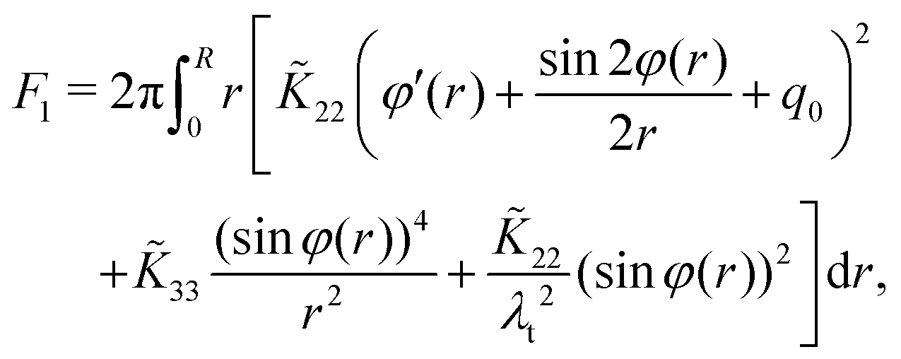 | (3) |
 | (4) |
 | (5) |
 | (6) |
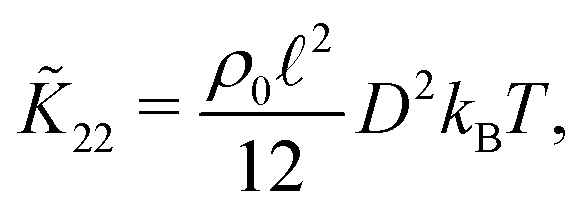
= L/D the rod aspect ratio and ρ0 the 2d number density of rods within the membrane.
The approximated free energy F1 is then minimised with respect to the twist angle profile, φ(r), keeping the radius fixed. Results for different membrane radii R, penetration depths λt, and inverse cholesteric pitches q0, can be found in ref. 22, where the minimisation was done with a simulated annealing method and a discretised twist angle profile.
3.2 Version II
The second attempt takes the membrane as a 3d object with an explicit surface, similar to the treatment of tactoids in ref. 25 or membranes in the one-constant approximation in ref. 14. I.e. the free energy terms include the local height of the membrane, Lcos![[thin space (1/6-em)]](https://www.rsc.org/images/entities/char_2009.gif) φ(r), the surface area (cover surface Sc and lateral surface S), and an anchoring strength w accounting for effects due to the anisotropy of the particles. The action of the depletants is translated to a surface tension τ, and the associated surface energy is given by:
φ(r), the surface area (cover surface Sc and lateral surface S), and an anchoring strength w accounting for effects due to the anisotropy of the particles. The action of the depletants is translated to a surface tension τ, and the associated surface energy is given by:where

![[q with combining right harpoon above (vector)]](https://www.rsc.org/images/entities/i_char_0071_20d1.gif) () denotes the surface normal at position . In addition, also the saddle-splay contribution F24 is included, which is related to director field deformations at the surface that are usually neglected in bulk systems,
() denotes the surface normal at position . In addition, also the saddle-splay contribution F24 is included, which is related to director field deformations at the surface that are usually neglected in bulk systems,with K22 + K24 the corresponding (constant) proportionality factor.

Since the membrane is a single layer of rods with centres fixed to a plane, the surface is given by the local height, which is defined by the twist angle profile, h() = Lcosφ(). The local height is also used to calculate the surface normal (). Assuming circular symmetry again, the resulting approximation of the free energy reads:
 | (7) |
| =:K22F22 + K33F33 + (K22 + K24)F24 + τSc + τwSw + τS. | (8) |
The elastic constants K22 and K33 are different from those in the first attempt, where the system is treated as an effective two-dimensional one. The approximated free energy F2 will be minimised for a given set of the constants (Kij, τ, w) by varying parameters of an explicit form of the twist angle profile φ(r). We minimise F2 under the assumption of a constant membrane volume. Strictly speaking, the pressure is constant and given by the density of the depletant gas so that the volume fluctuates about its average value. However, the constant volume assumption is sufficient for our purposes because we will compare with averaged simulation results, and the average volume is constant. F2 is computed using numerical integration routines of Mathematica.
In this paper, we use version II to extract the Frank elastic constants by comparing theoretical and simulated twist angle profiles. And we use version I to determine the inverse cholesteric pitch and the twist penetration depth, likewise by comparing theoretical and simulation results.
4 Results
4.1 Simulation results
The parameters that were varied in this Monte Carlo simulation study are the rod aspect ratio = L/D, the number of rods N, the number density of Asakura-Oosawa (AO) spheres ρD, and the chiral strength ε.
An important quantity to measure is the twist angle profile φ(r). It describes the angle between the membrane normal and the average nematic director at a distance r from the membrane's centre. Most of the twist angle profiles can be described by three parameters: the radius of the membrane, R, the twist angle at the rim of the membrane, φ0, and an exponent α that determines the slope of the profile at the rim. So we take the functional form to be:
 | (9) |
To calculate the twist angle profile from the simulated configurations, we need the local nematic director (). The nematic director of a collection of uniaxial particles is the eigenvector that belongs to the largest eigenvalue of the ordering tensor Qij:
 k is the unit vector along the axis of particle k, and Nc is the number of particles. The largest eigenvalue itself is the nematic order parameter S2. In bulk, S2 is close to 1 for a nematic phase and 0 for an isotropic phase. For the finite-sized membranes, it will be close to 1 if the membrane is untwisted and smaller than one if there is a double-twist. If the twist happens only close to the rim (curved twist angle profile), S2 will be larger compared to the case of a homogeneously twisted membrane (linear profile). Exemplary twist angle profiles are shown in Fig. 6 in Section 4.2, where the comparison to theoretical predictions is discussed.
To finally be able to fit eqn (9) to the simulation results and to calculate the two-dimensional number density of rods in the membrane, ρ0 = N/(πR2), we need to define the radius R. Because the membranes are not perfectly circular and the rod-depletant interface is not sharp, we employ the following procedure. We measure the radial number density profile ρr(d) = Np(d)/Vr(d), where d is the binned radial in-plane coordinate with respect to the membrane's centre of mass. Vr(d) is the volume of a thin cylindrical ring with radii d − Δd/2 and d + Δd/2; both bin width and height of the cylindrical ring are set to Δd = 0.1D. The quantity Np(d) represents the reduced number of segments with distance in [d − Δd/2, d + Δd/2) from the membrane's centre. We introduce this quantity to account for the occupied space of the whole rods and not only of their centres of mass (keep in mind that an upright and a lying rod look the same when only the centre of mass is considered). Therefore the rods are divided into L/D + 1 segments of equal width. The reduced number of segments in a bin is the actual number of segments divided by L/D + 1 to assure the correct scaling of the number density. We fit the rod-depletant interface to a hyperbolic tangent t(d) = a(tanh(c(b − d)) + 1), with fit parameters a, b and c, and use this to find the equal-mass point by numerical integration in cylindrical coordinates. Equal-mass means that the amount of material missing on the material-rich side equals the surplus material on the material-poor side compared to a sharp interface. I.e. we solve

We focus on liquid-like membranes that show a homogeneous double twist, as, for example, seen in Fig. 1. To achieve this, one has to set the depletant concentration in a suitable range. Stable membranes exist when a demixing of the binary system (hard rods and AO spheres) minimises the system's free energy. If the number density of depletants is very low, the system starts to mix, and the membrane falls apart (unstable region). On the other end, when the depletant density is very high, the system undergoes an ordering transition, finally resulting in a hexagonal platelet of parallel rods. This transition is also found in experimental systems composed of fd viruses and Dextran as nonabsorbing depleting agent.9 A discussion about the intermediate states found in our simulations is given in the Appendix A.1. For the main text, we take depletant concentrations that result in liquid-like membranes. We choose two example sets of simulations to examine further details; one with a fixed number of rods and varying depletant densities and one with a fixed depletant density and a varying number of rods.
![[small script l]](https://www.rsc.org/images/entities/b_char_e146.gif) = 20, N = 2209.
We begin by considering the achiral case, ε = 0 kBT. The two-dimensional number density of rods (short: rod density) in the membrane, ρ0 = N/(πR2), can be tuned over a wide range (≈0.3–0.7D−2) by adapting the depletant density, as can be seen in Fig. 2(a). As the rod density increases, the edge twist angle decreases, i.e., the membranes appear less twisted, cf.Fig. 3(a), which comes from the incommensurability of dense packing and tilting of rods. The simulation with the lowest depletant density deviates from this trend. At this point, we are close to the limit of stability before the membranes fall apart. Also, the curvature parameter α is smaller than 1 in that case (Fig. 3(b)), resulting from a negative curvature of the twist angle profile. It is not within the scope of this paper to study the dissolution of membranes, so we did not investigate the low ρD limit in more detail. Due to the decreasing twist, the nematic order parameter increases with increasing depletant density (curve with ε = 0 kBT in Fig. 2(b)). Thus, it is easy to change the density of colloidal membranes for practical purposes and, with that, also their stiffness and internal structure by adding more or less depleting agents. Similar effects can be expected by changing the strength of the depletant interaction due to variable depletant sizes, which can, for example, be achieved by using thermoresponsive depletants that adjust their size upon varying the temperature.34
= 20, N = 2209.
We begin by considering the achiral case, ε = 0 kBT. The two-dimensional number density of rods (short: rod density) in the membrane, ρ0 = N/(πR2), can be tuned over a wide range (≈0.3–0.7D−2) by adapting the depletant density, as can be seen in Fig. 2(a). As the rod density increases, the edge twist angle decreases, i.e., the membranes appear less twisted, cf.Fig. 3(a), which comes from the incommensurability of dense packing and tilting of rods. The simulation with the lowest depletant density deviates from this trend. At this point, we are close to the limit of stability before the membranes fall apart. Also, the curvature parameter α is smaller than 1 in that case (Fig. 3(b)), resulting from a negative curvature of the twist angle profile. It is not within the scope of this paper to study the dissolution of membranes, so we did not investigate the low ρD limit in more detail. Due to the decreasing twist, the nematic order parameter increases with increasing depletant density (curve with ε = 0 kBT in Fig. 2(b)). Thus, it is easy to change the density of colloidal membranes for practical purposes and, with that, also their stiffness and internal structure by adding more or less depleting agents. Similar effects can be expected by changing the strength of the depletant interaction due to variable depletant sizes, which can, for example, be achieved by using thermoresponsive depletants that adjust their size upon varying the temperature.34
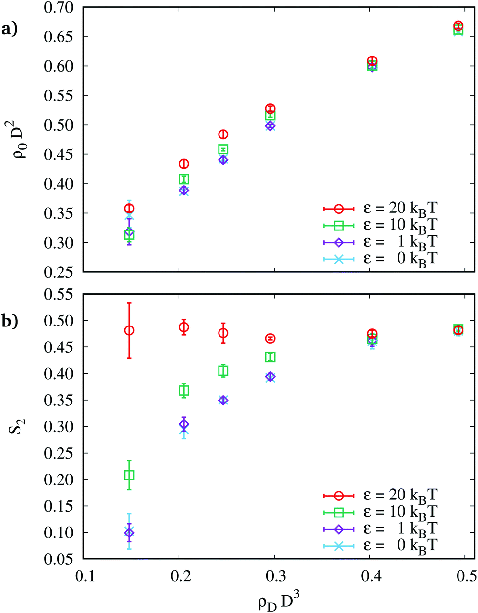 | ||
| Fig. 2 (a) Rod number density and (b) nematic order parameter vs. depletant density for different ε and = 20, N = 2209. Error bars depict the standard error of the mean from at least three independent simulation runs. | ||
 | ||
| Fig. 3 (a) Edge twist angle and (b) curvature parameter from fitting simulated twist angle profiles to eqn (9)vs. depletant density for different ε and = 20, N = 2209. Error bars depict the standard error of the mean from at least three independent simulation runs. | ||
A non-zero chiral strength has two effects: (i) the interaction between rods becomes attractive or repulsive depending on the angle that is embedded between their axes (see eqn (1), (ii) the nematic phase in bulk systems is replaced by a chiral nematic (or cholesteric) phase with a finite pitch; i.e. the nematic director rotates along an axis, and the pitch tells on which length it does a full rotation. This, qualitatively speaking, results in (i) a shift of ordering transitions, (ii) a more strongly twisted membrane, and (iii) an even greater variety of structures (see below).
When increasing the chiral strength, we find a change in the behaviour of the nematic order parameter versus the depletant density, cf.Fig. 2(b). For small ε, it increases with increasing density, but for ε = 20 kBT, S2 has much higher values for low ρD. For higher depletant densities, it coincides again with the values for lower ε. This originates from the different behaviour of α for ε = 20 kBT, cf.Fig. 3(b): a large value of α means that the twist happens mainly close to the membrane rim so that a large fraction of rods in the membrane centre is less twisted, resulting in a high value of S2 found for low densities. As expected, the edge twist angle and the curvature parameter increase with the chiral strength, cf.Fig. 3. Furthermore, due to the attractive nature of the interaction potential, the rod number density also slightly increases with increasing chiral strength. For high ρD, the curves for different ε in Fig. 2 merge because there the dominant interaction is the depletion interaction that suppresses the effects of the chiral interaction. Thus, to see an effect of a chiral interaction on the shape and structure of colloidal membranes, the depletant concentration must be chosen in a suitable range.
= 20, ρD = 0.25D−3.
For the rod density as a function of the number of rods, we observe two regimes: ρ0 decreases up to a size of about N = 3000 and increases again for larger membranes (Fig. 4(a)). The nematic order parameter behaves similar, but with a shift of the minimum to slightly smaller membranes (N = 2000, Fig. 4(b)). Besides, we find that for small membranes, the twist angle profile is almost linear, i.e., α ≈ 1, while for large membranes, it gets more and more curved so that the central part is virtually untwisted and the twist happens only close to the rim (this is illustrated for a chiral case in Fig. 6(a)). At the same time, the twist angle at the rim, φ0, increases with increasing size up to N ≈ 3000 and slightly decreases for larger membranes, cf.Fig. 5 which is discussed later on. If one could separate the effects from edge twist angle, profile curvature, and membrane size (in terms of the number of rods), one would expect the following: for fixed φ0 and profile shape, the order parameter increases with membrane size because more and more rods are only weakly twisted. For fixed membrane size and profile shape, the order parameter decreases with φ0. Furthermore, for fixed membrane size and φ0, the order parameter increases for stronger curved profiles. From these three effects, we can explain the two observed regimes for S2. We conclude that for N < 2000, the order parameter decreases due to the strong increase of the edge twist angle φ0, while the increase of S2 for larger N complies with the increasing size and curvature. Note: the somewhat larger error bar for N = 1600 and ε = 20 kBT is a result of one of the simulations having a membrane separated in two compartments. For a further discussion on this, see Section 4.5. Remark (not shown): for shorter rods, we find that the respective minimum of the order parameter is shifted to a smaller membrane size.
 | ||
| Fig. 4 (a) Rod number density and (b) nematic order parameter vs. number of rods within the membrane for different ε and = 20, ρD = 0.25D−3. Error bars depict the standard error of the mean from at least three independent simulation runs, except for N > 5000, where only 1–2 simulations were carried out. | ||
 | ||
| Fig. 5 (a) Edge twist angle and (b) curvature parameter from fitting simulated twist angle profiles to eqn (9)vs. number of rods within the membrane for different ε and = 20, ρD = 0.25D−3. Error bars depict the standard error of the mean from at least three independent simulation runs, except for N > 5000, where only 1–2 simulations were carried out. | ||
For chiral strengths ε ≤ 20 kBT, we find a reversal of the order parameter's behaviour with increasing chiral strength: for N ≤ 625 S2 decreases with ε and for N ≥ 900 S2 increases with ε, while the density increases with ε for all N. This again results from the combination of membrane size (given by N), edge twist angle (φ0), and curvature of the twist angle profile (given by α): for small N, the edge angle varies strongly with the chiral strength, while the curvature stays relatively unaffected, resulting in a decreasing nematic order parameter, cf.Fig. 5. However, for N around 1000–3000, the edge angle changes only weakly with ε, while the curvature increases, resulting in an increasing order parameter. Finally, for larger membranes, the twist angle again strongly depends on the chiral strength but not strong enough to compensate for the effect of the increase of α, so that S2 still increases with ε.
In conclusion, we have two valuable findings: we can tune density and nematic order parameter in a non-monotonic way by varying the numbers of rods in a membrane, and we can find a size where the response to a change in the interaction (changing ε or temperature T) is reversed. A brief evaluation of the potential energy in these systems is given in the Appendix A.2.
We now turn to the discussion of the theoretical predictions and their applications.
4.2 Comparison to theory version I
The twist angle profile that is predicted by version I of the approximation to the free energy is the one that minimises the elastic energy in eqn (3) for a given set of parameters. Some of the parameters can directly be inferred from simulations: the membrane radius R, the two-dimensional number density ρ0, and the aspect ratio of the rods. Only two parameters are left for which the mapping is not known precisely: the inverse cholesteric pitch q0 and the twist penetration depth λt. How they are extracted from the simulations, under the assumption that the theory applies to the simulated system, is described below.
But first, we show that similar trends as found in ref. 22 appear in our simulations (cf.Fig. 2 in ref. 22). The parameters tuned in the simulations are the number of rods in the membrane N, the number density of depletants ρD, and the interaction strength between rods ε. The radius is found from the simulations using the density profile as described in Subsection 4.1. The trends found in our simulations are as follows:
(i) The twisted region moves to the membrane edge with increasing membrane size, Fig. 6(a). This is in accord with ref. 22.
 | ||
| Fig. 6 Twist angle profiles. The angle is scaled to the angle at the edge, φ0, and the distance from the centre is scaled to the membrane radius R. (a) different N and = 20, ε = 20 kBT, ρD = 0.25D−3, (b) different ρD and = 20, ε = 20 kBT, N = 2209, (c) different N and ε and = 20, ρD = 0.25D−3. The same graphs with different axes scaling are shown in the Appendix A.3. | ||
(ii) The twist angle profile's curvature decreases with increasing depletant concentration, Fig. 6(b). This hints at a proportionality between ρD and the twist penetration depth λt, for which the same trend is found in ref. 22. The relation is not obvious but connected to the fact that we cannot increase the depletant density without increasing the rod density as well (up to maximum packing, of course).
(iii) The chiral strength affects the twist angle profile: the curvature increases the larger the chiral strength, Fig. 6(c). This is not seen in Fig. 2 of ref. 22, but this might be related to the choice of parameters in a regime that is less affected by the chiral interaction strength. We provide the graphs of Fig. 6 with different axes scaling in the Appendix A.3.
Returning to the comparison to the predictions obtained by version I, the inverse pitch and penetration depth are found by minimising squared residuals between simulated and predicted twist angle profiles. In detail, this means.
• Run a simulation with parameters (l, N, ρD, ε).
• Compute the twist angle profile φsim(r) and determine the membrane radius R and density ρ0.
• Choose the remaining parameters λt and q0; e.g. on a lattice in a predefined region.
• Find the twist angle profile φth1(r) that minimises eqn (3) for each pair of (q0, λt); e.g. by simulated annealing.
• Compute the sum of squared residuals  where rk are discretised distances.†
• Find the pair of (q0, λt) that minimises the squared residuals S(q0, λt).
The expected behaviour is that q0 is proportional to ε; especially the case ε = 0 should correspond to q0 = 0. λt is expected to relate to the densities of both, rods and depletants.
Fig. 7 shows the dependence of q0 on ε for different membrane sizes and fixed depletant concentration. The expected trend is affirmed: |q0| increases with increasing ε. However, for ε = 0 kBT we do not find q0 = 0/D. The reason is that for q0 = 0/Deqn (3) is minimised for φ(r) = 0, i.e. no twist at all. In contrast, for ε = 0, the simulated membrane still twists to reduce its surface. This discrepancy enhances the smaller the membrane is, and so we can define a limitation of the theory: achiral and small systems cannot be captured by eqn (3). A size dependence of q0 is also found for ε ≠ 0 kBT. In general, this size dependence is not only related to the surface-to-volume ratio of a membrane but also to the size dependence of the rod number density. The latter influences the cholesteric pitch and can be non-monotonic, as, e.g. in the examples shown in Fig. 4(a).
 | ||
| Fig. 7 Inverse cholesteric pitch from mapping results of theory I to results of simulations with different N and ε and = 20, ρD = 0.25D−3. q0 is found from minimising squared residues of theoretical and simulated twist angle profiles. Error bars denote the range of values found from different runs. | ||
Fig. 8 shows the dependence of λt on ρD for different chiral strengths and a fixed membrane size. With increasing chirality, the penetration depth decreases, which is related to lowering the cholesteric pitch (which is a characteristic length scale of chiral nematic systems). The behaviour of λtvs. the depletant concentration depends on the chiral strength: the penetration depth decreases slightly with ρD for small ε and increases with ρD for large ε. Similar differences were obtained for the nematic order parameter (Fig. 2(b)) and the twist angle profile (Fig. 3). Thus, we conclude that the behaviour of λt is also related to the behaviour of the membrane curvature, Fig. 3(b).
 | ||
| Fig. 8 Twist penetration depth from mapping results of theory I to results of simulations with different ρD and ε and = 20, N = 2209. λt is found from minimising squared residues of theoretical and simulated twist angle profiles. Error bars denote the range of values found from different runs. | ||
In summary, version I comes with explicit expressions for elastic constants and leads to reasonable results when compared to simulations unless the membranes get too small or are composed of achiral rods. To get a deeper insight into the different contributions to a membrane's free energy, we base our further discussions on the more general version II of the theoretical approximation.
4.3 Discussion of terms in theory version II
To examine the different free energy contributions in version II of the approximation to the free energy, eqn (8), we chose a specific form for the twist angle profile that matches the findings from the simulations: φ(r) = φ0(r/R)α, cf.eqn (9). We assume that the membrane volume is fixed by the number of rods within the membrane and the depletant density. Hence, when we want to find the twist angle profile that minimises the free energy in eqn (8) for a specific set of parameters, we need to fix the volume V. This, in turn, means that the radius depends on the currently chosen twist angle profile and is found from | (10) |
In the following, we describe how the different terms in eqn (8) change with the twist angle profile for a constant volume of V = 10000D3 (if not stated differently).
Fig. 9 shows the twist contribution F22 for different parameters. It is the only term that changes its behaviour when a chiral interaction is turned on. It is clear that in the achiral case (q0 = 0, Fig. 9(a)) any deviation from the uniform, untwisted state, φ(r) = φ0 = 0, is penalised by an increase in the energy. However, if the system needs to twist, a linear twist angle profile (α = 1) is favoured over a curved one (α > 1). In the chiral case (q0 ≠ 0, Fig. 9(b) and (c)) the twist contribution shows a minimum at φ0 > 0, as expected. The minimum shifts to larger angles with an increasing absolute value of the inverse pitch q0 (Fig. 9(b)). This is the same as in bulk: the smaller the cholesteric pitch, the stronger the system needs to twist. The volume of the membrane also affects the position of the minimum (Fig. 9(c)): it roughly scales with  which is proportional to the membrane radius.
 | ||
| Fig. 9 Twist contribution to the free energy in eqn (8). (a) q0 = 0/D, = 10, V = 10000D3 and different α, (b) α = 4, = 10, V = 10000D3 and different q0, (c) α = 4, q0 = −0.04/D, = 10 and different V. | ||
Fig. 10 shows the bend contribution for different α, which reduces to

 | ||
| Fig. 10 Bend contribution to the free energy in eqn (8) for different α and = 10. | ||
Fig. 11 shows the saddle-splay contribution

 | ||
| Fig. 11 Saddle-splay contribution to the free energy in eqn (8) for different α and = 10. | ||
Fig. 12 shows the cover surface area Sc for different combinations of α, and V. Any twist increases the cover surface area, which is one part of the interface between the membrane rods and the depletants. The rise is strongest for small α (linear profile), long rods and small membrane volumes (note: the graphs show Sc/V because Sc(φ0 = 0) ∝ V). So this contribution also drives the membrane to an untwisted state. In contrast, the lateral surface area S decreases (to zero) with increasing twist angle at the rim, Fig. 13. It slightly depends on α because the radius depends on α, and it increases proportionally to  and .
and .
 | ||
| Fig. 12 Cover surface area for different combinations of α, and V. | ||
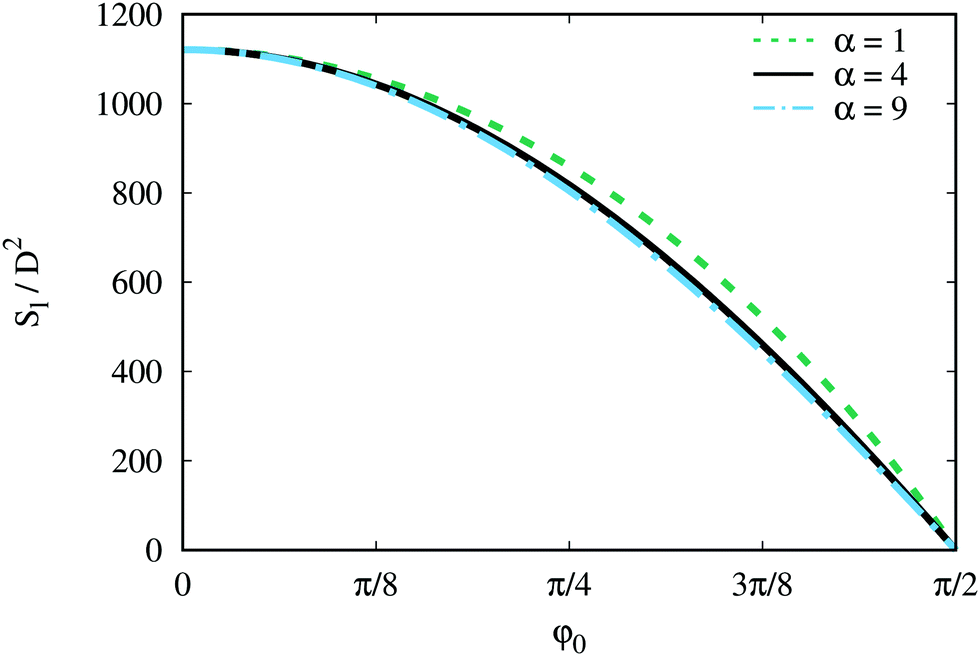 | ||
Fig. 13 Lateral surface for different α and = 10. (The scaling  is not extra shown). is not extra shown). | ||
Finally, the surface anchoring contribution Sw has its minimum at φ0 = π/2, Fig. 14. It is smallest for small α (linear profile), long rods and small membrane volumes. This behaviour is obvious when considering that the angle between the local nematic director and the local surface normal must everywhere be as large as possible to reduce the surface anchoring contribution. (Note: for Sw(φ0 = 0), the same scaling applies as for Sc).
 | ||
| Fig. 14 Surface anchoring contribution to the free energy eqn (8) for different combinations of α, and V. | ||
Table (1) summarises the impact of all contributions on φ0 and α. With this at hand, there appear (at least) two applications: (i) if the elastic constants Kij, the inverse pitch q0, the anchoring strength w and the interfacial tension τ and their dependencies on rod and depletant densities are known, one can tune the shape of colloidal membranes target-oriented. (ii) If the twist angle profile is measured (in experiments or simulations), one can deduce a set of prefactors (Kij, τ, w) for which the measured profile minimises the membrane free energy. Thus, this defines a complementary way for determining elastic constants, interfacial tension and anchoring strength‡ (and even the cholesteric pitch) of (chiral) liquid crystalline systems.
| F 22 | F 33 | F 24 | S c |
S
|
S w | |
|---|---|---|---|---|---|---|
pf: prefactors for the different contributions to the free energy in eqn (8). V and : scaling ranges of the contributions with volume and rod aspect ratio. The two values for F22 refer to q0 = 0 and q0 ≠ 0. ⇕ means that no specific scaling is found, but depends on q0. “—” means no dependence. φ0 and α: impact of the contributions on the twist angle profile defined by eqn (9); the radius is given by a fixed volume. The two values for F22 refer to q0 = 0 and q0 ≠ 0.⇓ (⇑) means that the contribution pulls the value of φ0 or α down (up) to minimise the energy penalty.  is a minimum that depends on the chirality given by q0 and φ0 is pulled towards is a minimum that depends on the chirality given by q0 and φ0 is pulled towards  . “—” means no effect. . “—” means no effect. |
||||||
| pf | K 22 | K 33 | K 22 + K24 | τ | τ | τw |
| V | —; ⇕ | — | — | V 0.5⋯1.0 | V 0.5 | V 1.5⋯1.0 |
|
1.0; ⇕ |
1.0 |
1.0 |
−1.0⋯0.5 |
0.5 |
−1.0⋯−2.5 |
| φ 0 | ⇓;  |
⇓ | ⇓ | ⇓ | ⇑ | ⇑ |
| α | ⇓; ⇓ | ⇑ | — | ⇑ | ⇑ | ⇓ |
4.4 Elastic constants from comparison of simulation and theory
A common way to determine elastic constants from simulations is to sample director field fluctuations at different length scales. This usually involves transformations to and calculations in Fourier space and a polynomial fit to finally get the values of the constants.35 Another route to finding elastic constants uses direct correlation functions and the Poniewierski-Stecki theory.36,37 To get the Frank elastic constants from experiments common methods are light scattering32,38,39 and using the Fréedericksz transition.40,41Here, we test a different approach to map theory and simulation results. As described in the previous subsection, it is possible to find a set of elastic constants and interface parameters for the colloidal membrane by comparing the twist angle profile found in simulations to the one predicted by theory. We assume that the simulation profiles fit the quite simple form eqn (9). If this would not be the case, another functional form could be chosen, and the analysis in the previous subsection would be repeated. However, we suppose that the trends do not depend on the specific form used to describe the twist angle profile as long as the characteristics are similar.
To get elastic constants from the comparison of simulation and theory, we propose the following procedure:
• Run a simulation with parameters (l, N, ρD, ε).
• Compute the twist angle profile φsim(r), determine the membrane radius R, and fit the profile to eqn (9) to get α and φ0.
• Compute the volume that will be kept fixed using the profile and membrane radius from the simulation in eqn (10).
• Choose an initial guess for the set of parameters (Kij, τ, w) and find the twist angle profile φth2(r) that minimises the free energy approximated by eqn (8).
• Minimise the difference between φsim(r) and φth2(r) by adapting the parameters (Kij, τ, w). We compare the twist angle profiles pertaining to the values of φ0 and α, but one could also define other similarity measures.
The set of parameters (Kij, τ, w) that lead to a specific twist angle profile is, in general, not unique. Therefore it is inevitable to (i) have some other input (e.g. parameters that are already known or parameter regions that can safely be excluded or results from related systems) and (ii) do validity checks. For example, in earlier studies of achiral hard spherocylinders of aspect ratio = 10 that form nematic tactoids in a bath of Asakura-Oosawa spheres, surface tension and anchoring strength were estimated to be: τ = 0.07kBT/D2 and w = 0.8.42 Because the minimum of eqn (8) is independent of an overall factor, we can only find ratios of energy parameters; therefore, we set K22 to be the unit of all other elastic constants and the surface tension (multiplied by D). With the assumptions made in ref. 42 this translates the value 0.07kBT/D2 to τ = 0.23K22/D. For a membrane composed of N = 3600 hard (achiral) rods of aspect ratio = 10 and depletant density ρD = 0.46D−3, we find parameter sets with reasonably close values of τ and w: 0.98 < w < 1.23 for 0.16 < τD/K22 < 0.42. We provide ranges and not single values because several sets of parameters result in the same twist angle profile. Within these ranges we find possible values of K33 to be: 5 < K33/K22 < 107, and of K24 to be: 1.4 < K24/K22 < 14.4. These ranges are somewhat reasonable but not very narrow. So we go on by assuming that ε does not affect w.§ We also know that for positive ε, the inverse pitch q0 must be negative, and its magnitude increases with ε. Therefore we compare parameter sets for ε = 0, 5, 9, 10 kBT and otherwise same simulation parameters, and find the following behaviours in the narrow range 1.068 < w < 1.078:
q 0 decreases from 0/D to −0.22/D at ε = 10 kBT (with approximately ∝ − ε4); τD/K22 increases from 0.217 to 0.267 (with approximately ∝ε6); K33/K22 increases from 20 to 61 (with approximately ∝ε2–ε3); and K24/K22 increases from 5 to 24 (with approximately ∝ε4). Note that the given values and power laws are rough estimates from the mapping results; for each of the four ε values, a few parameter values were collected, and the corresponding fits to power laws were assessed. This part should merely demonstrate the procedure. The correctness of functional forms for the quantities of interest can always be improved by analysing more twist angle profiles. For experimental studies, the first two points of the procedure need to be adapted. However, the general procedure should work similarly well, and it should also be suitable for determining elastic constants and interfacial properties of experimental systems.
4.5 Transition to two-dimensional blue phase
What happens when the chiral strength is increased to very high values? The equilibrium bulk cholesteric pitch is inversely proportional to the chiral strength, i.e. with increasing chirality, the rods tend to increase the angle between successive layers. In a colloidal membrane, the rods cannot tilt arbitrarily. The twist angle is largest at the rim and decreases monotonically to zero in the centre. However, if the chiral potential is strong enough, the membrane starts to form substructures to lower its overall free energy. Using the straightforward Metropolis-Monte-Carlo technique, we find various structures, but we do not verify whether they are stable or meta-stable in this paper. To do this, one needs other simulation approaches, but this is not the scope of the current study. Also, fixing the rods to a plane influences the substructures; if moving away from the plane would be allowed, the rods would escape to the third dimension and form complex 3D structures. This scenario would be better comparable to existing experiments, where an increasing chiral interaction leads to the formation of a rippled membrane edge and the transition to twisted ribbons.5 We are aware that the fixed-particle setup chosen for the current study cannot account for such a transition and that the findings presented in this section are specific to our (artificial) simulation setup. For a realisation, one could think about fixing chiral molecules to a fluid–fluid interface; but we are not aware of experiments on the formation of disk-shaped membranes in such a setup.We find several types of structures that depend on the initial condition and the rod aspect ratio and begin the discussion by describing our findings. The options used for initial conditions are: (i) untwisted membrane, (ii) twisted membrane without substructure, (iii) twisted membrane with substructure. The resulting structure does also depend on the magnitude of the chiral strength.
There is a critical chiral strength ε*, above which substructures appear. If the chiral strength is close to that (and the initial condition is (i) or (ii)), it is likely to find a membrane that twists towards the rim, as for lower chiral strength, but starts to divide in the centre (Fig. 15(a) and (c)).
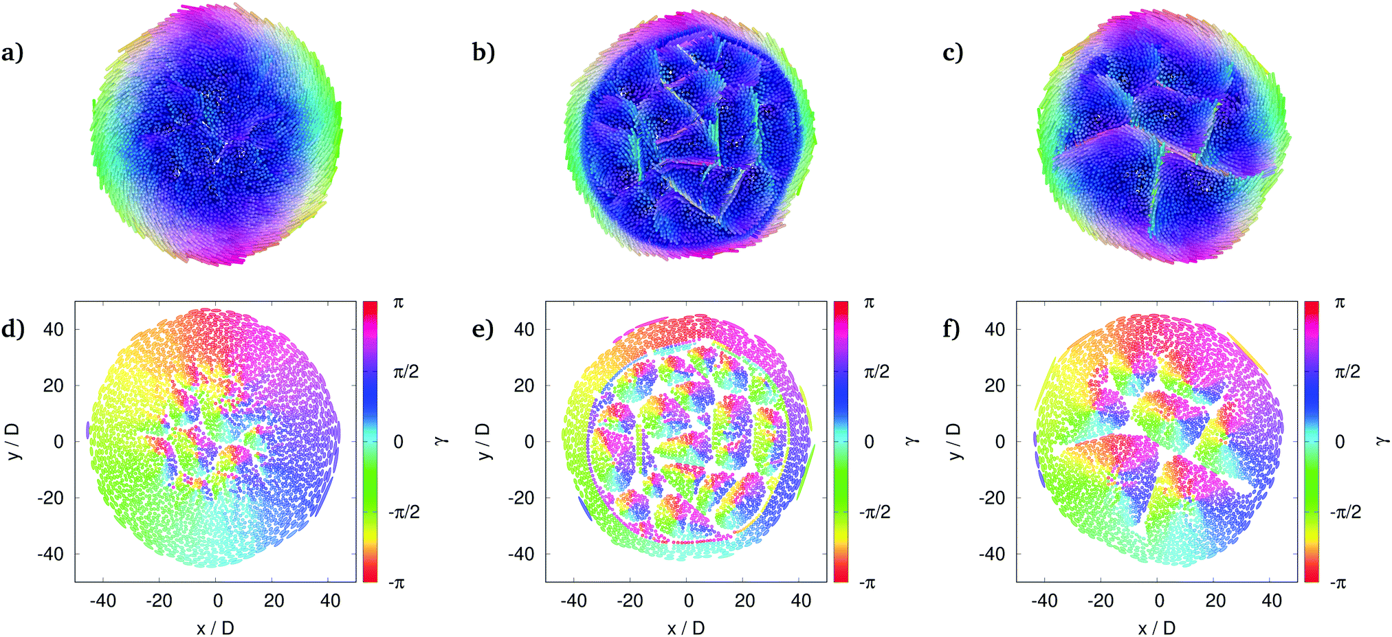 | ||
| Fig. 15 Different substructures for the same set of parameters (N = 3136, = 20, ε = 25 kBT, ρD = 0.25D−3). (a) and (d) Sub-twists start to form in the central part but are not fully developed. (b) and (e) An outer twisted ring is separated from inner sub-twists by a few layers of weakly twisted rods. (c) and (f) Developed sub-twists merge at the rim. The lowest potential energy is found for structure (b), the highest one for structure (c). For the membrane nematic order parameter, the inverse order applies. The upper panel shows rendered snapshots of the rods in the membranes, where the colour-coding indicates the rods' orientation. The lower panel shows cuts through the fixed plane so that tilted rods are shown by ellipses, and the colour-coding indicates the polar angle γ of the projection of the rods onto the plane. Double(sub)twists are therefore seen as objects including the whole colour spectrum. | ||
For slightly larger chirality, the membrane entirely separates into a few large and twisted compartments (not shown).
Starting from (ii) and increasing ε much beyond the critical value, the membrane separates into a twisted outer ring and an inner part that contains so-called sub-twists. Taking such a configuration as an initial condition for a simulation with a smaller chirality (but still larger than ε*), we find that the ring plus sub-twist structure is maintained (Fig. 15(b)). The rods in the ring's innermost and in the adjacent layer strongly decrease the potential energy by enclosing a large angle.
Starting from (i), on the other hand, leads to an arrangement of sub-twists that fills the total membrane area (Fig. 16), and can be regarded as a two-dimensional blue phase, but not necessarily with hexagonal structure as it was found in ref. 28. A hexagonal order would not be easy to achieve because the sub-twists are also not perfectly monodisperse in size. The size and number of sub-twists depend on ε, as can be seen by the three examples in Fig. 16. Increasing the chiral strength decreases the sub-twist size and hence increases their number.
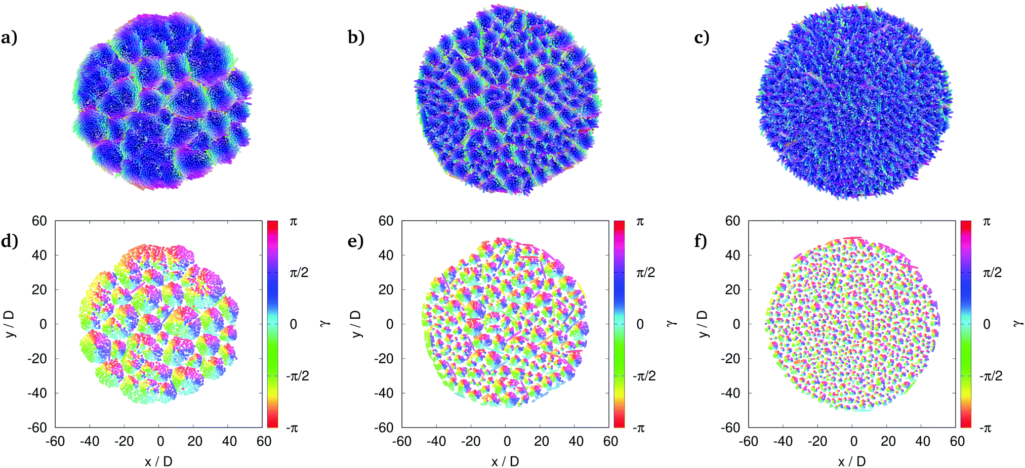 | ||
| Fig. 16 Sub-twist arrangement for different chiral strengths (N = 3600, = 10, ρD = 0.46D−3). (a) and (d) ε = 15 kBT, (b) and (e) ε = 25 kBT, (c) and (f) ε = 35 kBT. For too strong chiral interactions (c) sub-twists can hardly be defined anymore. Upper and lower panel as for Fig. 15. | ||
In general, the ring plus central part structure frequently appears for longer rods ( = 20), whereas the membrane usually fully decomposes to sub-twists for shorter ones. Also, the critical chiral strength for forming substructures increases with increasing rod aspect ratio.
To determine the critical chiral strength, one can, for example, find the point where the slope of the reduced potential energy as a function of chiral strength changes, as can be seen in Fig. 17 for = 20 and ρD = 0.25D−3, where the critical chiral strength is about ε* = 22 kBT. The change of the slope can be explained through the following considerations. From a theoretical point of view and regarding the different free energy terms, creating substructures has several effects:
 | ||
| Fig. 17 Reduced energy per particle vs. chiral strength for different N and = 20, ρD = 0.25D−3. Error bars depict the standard error of the mean from at least three independent simulation runs. | ||
(i) The overall surface is increased. There are many interfaces, and interfaces usually cost free energy.
(ii) But in this system, the potential energy decreases, especially at the interfaces, where adjacent rods from different sub-twists can have a larger mutual angle than the adjacent rods within the sub-twist.
(iii) By reducing the length scale over which deformations occur, the elastic energy is increased.
Above the critical chiral strength ε*, the enhanced elastic deformation and surface free energy is outweighed by the overall decrease of the chiral potential energy due to substructure formation. The membrane size does not affect the critical chiral strength. It does, however, influence the standard error of the mean of the energy from independent simulation runs. This originates from the lower number of possible substructures in small membranes, where a slight change in composition, e.g. from two to three substructures, leads to a large change in energy.
For possible applications of the substructure formation, it will be necessary to improve the control of the sub-twists' size and distribution.
5 Conclusion
We studied the behaviour of colloidal membranes composed of chiral rod-like particles by Monte Carlo simulation and compared our observations to two versions of an elastic theory. The typical form of such membranes is a one-layer thick double-twist cylinder showing circular symmetry. It is described by a twist angle profile, which is used to test the validity of different theoretical approaches. The profile depends on various parameters: the number and aspect ratio of rods, the strength of the chiral interaction, and the number density of the depleting agents. Qualitatively, the behaviour (trends with a change of parameters) is well described by both versions of the theory. The difference between the models (besides additional terms) is that the first uses the microscopic parameters from the simulation (only two parameters needed to be matched). In contrast, in the second version, all elastic and surface constants were used to map the theoretical profiles to those from simulations. One of the main take-home messages is that with the latter, we provide a method to determine Frank elastic constants, surface tension and anchoring strength from observing configurations of quasi-two-dimensional colloidal membranes. Knowledge of these quantities is, on the one hand, interesting from a theoretical (basic research) point of view and, on the other hand, essential for material design and engineering. The method is not restricted to simulated systems but may be used for experiments similarly; one just needs to measure the twist angle profile for several configurations, as was done, for example, in ref. 43. Thus, we think that the proposed procedure is applicable to experiments as a complementary method for determining elastic constants. We hope that our approach will stimulate more investigations in this direction.There is a transition to more complex structures for high chiral strengths, including rings and sub-twists (array of double-twists), where the latter is reminiscent of a two-dimensional blue phase. A rod aspect ratio dependent critical chiral strength for substructure formation was found from a change in the reduced potential energy behaviour.
We also found a distorted hexagonal lattice structure that, to our knowledge, has not been described before, and it would be interesting to study in more detail which kinds of transitions this system undergoes.
Conflicts of interest
There are no conflicts to declare.A Appendix
A.1 High density states
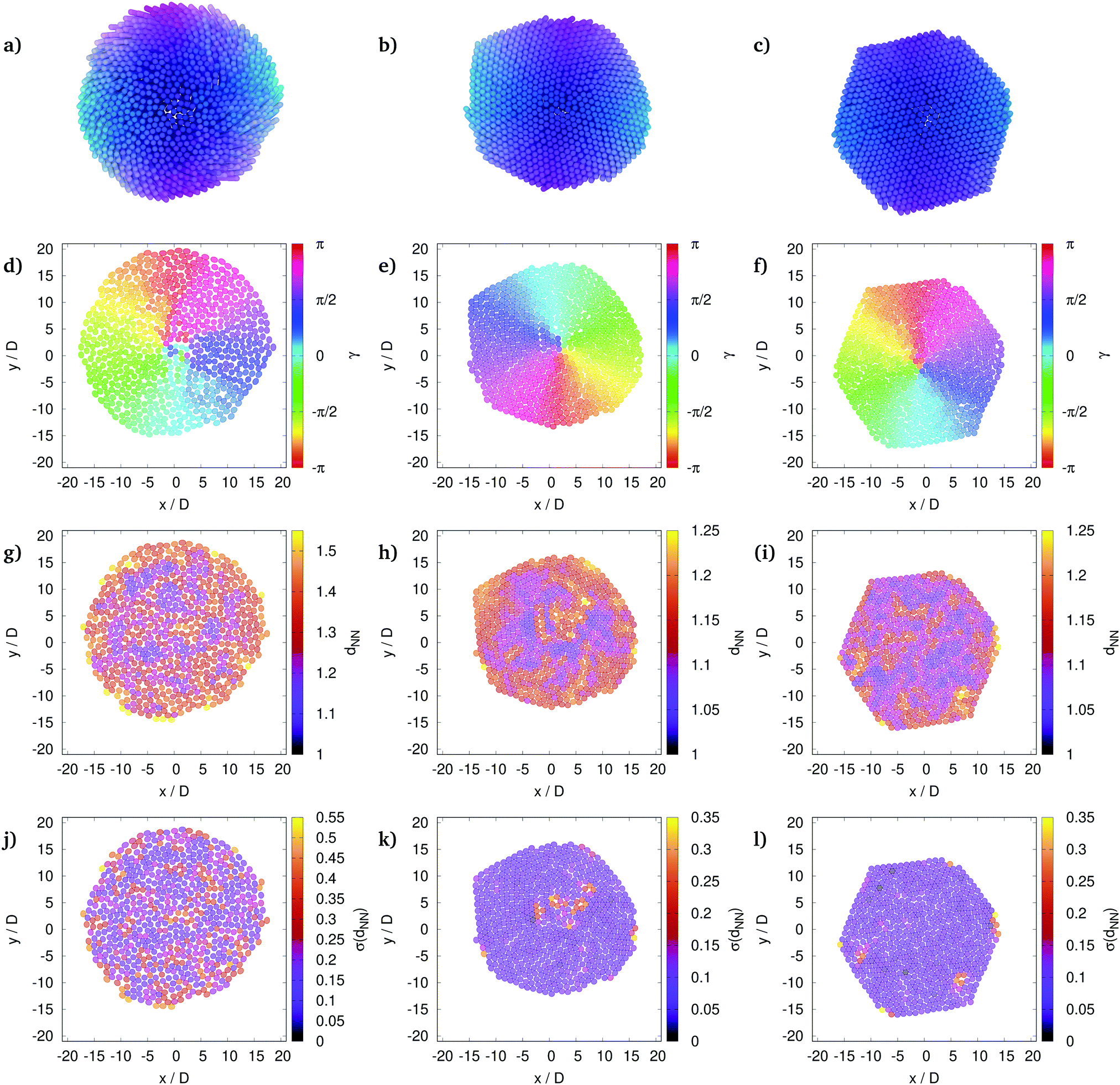
In the main text, we focus on twisted membranes in the liquid state; an example is shown in the first column of Fig. 19. The system shows short-range translational order and a double-twist director field in this state. By increasing the depletant density, we find a special intermediate state, before the system forms a perfect crystalline state. This intermediate state has a distorted hexagonal lattice (DHL) and a double-twist director field. DHL means the rods arrange on a lattice, but depending on their twist angle, the distances between centres of mass need to vary. This is best seen by cutting the system at the plane to which the centres of mass are fixed, cf.Fig. 19(d)–(f). Upright (untwisted) rods look like disks in this view, while tilted rods appear as ellipses. I.e. in the centre, where rods are untwisted, we find hexagonally packed disks. On the other hand, towards the membrane edge, where rods get more tilted than in the centre, we find ellipses that are also packed densely but do not sit exactly on a hexagonal lattice. The different possible structures are depicted in Fig. 19 for a small membrane of weakly chiral rods. (Note: we noticed no significant difference between ε = 0 kBT and 1 kBT for other sets of parameters and assume this holds for the shown set as well.) In the main text, we focus on homogeneously twisted membranes as the one in the first column (liquid); the second column shows the newly described distorted hexagonal lattice (DHL), and the third column presents an example of a nearly hexagonal lattice (crystal). The panels visualise different aspects of the membranes. In the top row, rendered snapshots of the membranes are shown. Here the double-twist is visualised by orientation-dependent colouring. The second row presents cuts through the fixed plane as described above, and the colour code indicates the polar angles of the ellipses. From this panel it is evident that even the nearly hexagonally shaped membrane has a double-twisted director field. The colour code in the third row shows the average distance to the six nearest neighbours. This distance distinguishes the DHL and crystal states: for the former, the distance increases towards the membrane edge due to the tilting of rods, while for the latter, this distance is constant. The shown nearly hexagonal example does not have a constant value for the average neighbour distance, confirming the declaration as ‘nearly’ hexagonal because it is not in a perfect crystalline state. In the fourth row, the colour code indicates the standard deviation of the average distance (from row three). It highlights defects in the lattice structure and illustrates that DHL has defects preferably close to the centre, while in the nearly crystal state, they are found away from the centre. (A perfect crystal would not have any defect.) The different structures can be found in simulations with the same set of parameters, as can be seen from the examples in columns 2 and 3 of Fig. 19. However, it is not the scope of this paper to discuss the origin of the different cases and the transitions between them in more detail (e.g. regarding the type – first-order vs. Kosterlitz-Thouless-Halperin-Nelson-Young scenario). Because of the elliptical cross-section of tilted rods, known results for two-dimensional colloidal disk systems that show liquid, hexatic, and crystal phases44,45 cannot simply be transferred to the current system. However, they could be used in future studies to compare the findings.The upper panel shows rendered snapshots of the rods in the membranes. The colour-coding indicates the rods' orientation (blue: only z-component, red: only x-component, green: only y-component; mixed colours according to the ratio of components). Depleting agents (Asakura-Oosawa spheres) are not shown, but they form a dense cloud around the membranes. The second panel shows cuts through the fixed plane so that tilted rods are shown by ellipses, and the colour-coding indicates the polar angle γ of the projection of the rods onto the plane (the colour is not related to the length of the projection). Double-twists are therefore seen as objects that include the whole colour spectrum. In the third panel, the colour-coding shows the average distance to the six nearest neighbours dNN of each rod; the outermost layer of rods (having fewer nearest neighbours) is removed. For the DHL structure, this distance increases towards the membrane edge. For a perfect undistorted lattice, the distance would be constant. The lower panel shows the nearest neighbour distance's standard deviation, σ(dNN). With this, defects in the lattice structures are highlighted.
A.2 Potential energy of twisted membranes
A non-zero chiral strength allows measuring the potential energy of the system, which gives further hints for understanding the system's behaviour. Fig. 18 shows the reduced energy per particle, U/(Nε), for example II, where U is the sum of all pair interactions given by eqn (1). With increasing membrane size, a large fraction of the system is untwisted, which is unfavored by the interaction potential and therefore increases its value. However, with increasing chiral strength ε, the reduced energy (note: already divided by ε) decreases. This can only mean that the gain of negative potential energy is large enough to compensate the loss of entropy due to the enhanced twisting and closer packing (the rod number density increases with increasing chiral strength, cf.Fig. 2(a) and 4(a)). The slight decrease of the energy for large membranes and high ε is due to the onset of emerging substructures discussed in Section 4.5. | ||
| Fig. 18 Reduced energy per particle vs. number of rods within the membrane for different ε and = 20, ρD = 0.25D−3. Error bars depict the standard error of the mean from at least three independent simulation runs, except for N > 5000, where only 1–2 simulations were carried out. | ||
 | ||
| Fig. 19 Different main structures found in simulations of weakly chiral rods (N = 729, = 10, ε = 1 kBT). (a), (d), (g) and (j) Short-range translational order and double-twist director field for ρD = 0.91D−3. (b), (e), (h) and (k) Distorted hexagonal lattice (DHL) and double-twist director field for ρD = 1.82D−3. (c), (f), (i) and (l) Nearly hexagonal lattice for ρD = 1.82D−3. Note that the system parameters for the latter two are the same. | ||
A.3 Alternative scaling of twist angle profiles
We present two versions of different scalings of Fig. 6 in Fig. 20 and 21.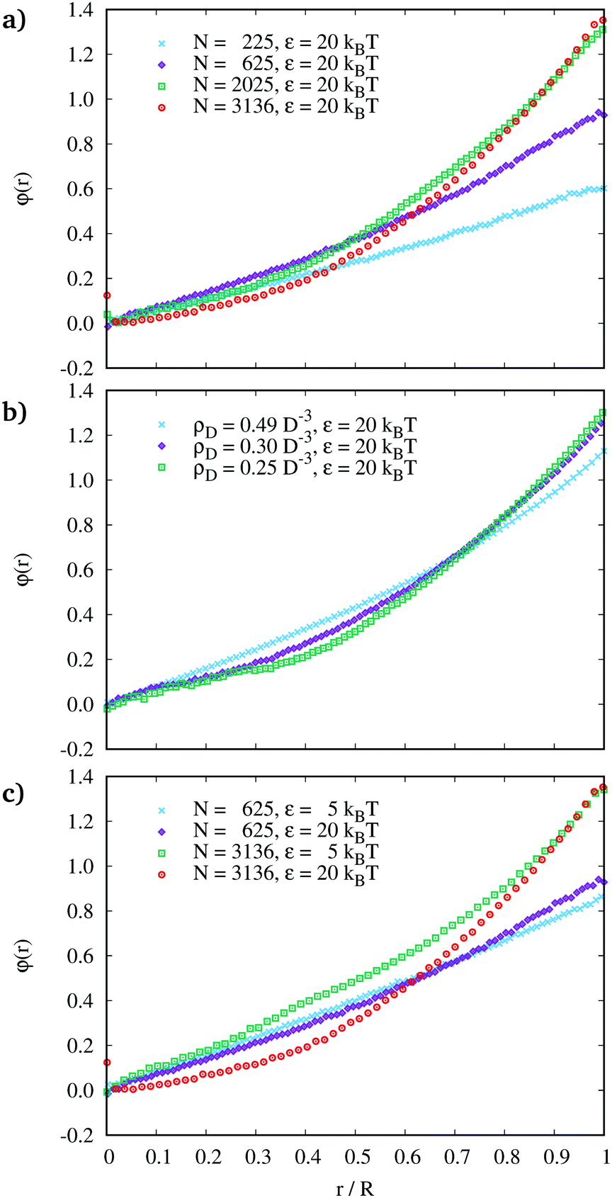 | ||
| Fig. 20 Twist angle profiles. The distance from the centre is scaled to the membrane radius R. (a) different N and = 20, ε = 20 kBT, ρD = 0.25D−3, (b) different ρD and = 20, ε = 20 kBT, N = 2209, (c) different N and ε and = 20, ρD = 0.25D−3. | ||
 | ||
| Fig. 21 Twist angle profiles (no rescaling). (a) different N and = 20, ε = 20 kBT, ρD = 0.25D−3, (b) different ρD and = 20, ε = 20 kBT, N = 2209, (c) different N and ε and = 20, ρD = 0.25D−3. | ||
Acknowledgements
The authors like to thank Tanja Schilling and Rik Wensink for helpful discussions and for providing basic code that we adapted for our purposes, and Paul van der Schoot, with whom a related system is studied. Support by the state of Baden-Württemberg through bwHPC and the German Research Foundation (DFG) through grant no INST 39/963-1 FUGG (bwForCluster NEMO) is acknowledged.References
- H. Kelker, Mol. Cryst. Liq. Cryst., 1973, 21, 1–48 CrossRef CAS.
- P. Palffy-Muhoray, Phys. Today, 2007, 60, 54 CrossRef CAS.
- Z. Dogic and S. Fraden, Curr. Opin. Colloid Interface Sci., 2006, 11, 47–55 CrossRef CAS.
- Z. Dogic, Front. Microbiol., 2016, 7, 1013 Search PubMed.
- T. Gibaud, J. Phys.: Condens. Matter, 2017, 29, 493003 CrossRef PubMed.
- B. Sung, A. de la Cotte and E. Grelet, Nat. Commun., 2018, 9, 1405 CrossRef PubMed.
- B. Sung, H. Wensink and E. Grelet, Soft Matter, 2019, 15, 9520–9527 RSC.
- Persistence of Vision Pty. Ltd. (2004) Persistence of Vision Raytracer (Version 3.6) [Computer software]. Retrieved from http://www.povray.org/download/.
- T. Gibaud and D. Constantin, J. Phys. Chem. Lett., 2018, 9, 4302–4307 CrossRef CAS PubMed.
- A. J. Balchunas, R. A. Cabanas, M. J. Zakhary, T. Gibaud, S. Fraden, P. Sharma, M. F. Hagan and Z. Dogic, Soft Matter, 2019, 15, 6791–6802 RSC.
- E. Barry and Z. Dogic, Proc. Natl. Acad. Sci. U. S. A., 2010, 107, 10348–10353 CrossRef CAS PubMed.
- M. J. Zakhary, T. Gibaud, C. Nadir Kaplan, E. Barry, R. Oldenbourg, R. B. Meyer and Z. Dogic, Nat. Commun., 2014, 5, 3063 CrossRef PubMed.
- C. Nadir Kaplan and R. B. Meyer, Soft Matter, 2014, 10, 4700–4710 RSC.
- L. Kang, T. Gibaud, Z. Dogic and T. C. Lubensky, Soft Matter, 2016, 12, 386–401 RSC.
- P. Sharma, A. Ward, T. Gibaud, M. F. Hagan and Z. Dogic, Nature, 2014, 513, 77–80 CrossRef CAS PubMed.
- S. Xie, M. F. Hagan and R. A. Pelcovits, Phys. Rev. E, 2016, 93, 032706 CrossRef PubMed.
- R. Sakhardande, S. Stanojeviea, A. Baskaran, A. Baskaran, M. F. Hagan and B. Chakraborty, Phys. Rev. E, 2017, 96, 012704 CrossRef PubMed.
- L. Kang and T. C. Lubensky, Proc. Natl. Acad. Sci. U. S. A., 2017, 114, E19–E27 CrossRef CAS PubMed.
- M. Siavashpouri, P. Sharma, J. Fung, M. F. Hagan and Z. Dogic, Soft Matter, 2019, 15, 7033–7042 RSC.
- J. M. Miller, C. Joshi, P. Sharma, A. Baskaran, G. M. Grason, M. F. Hagan and Z. Dogic, Proc. Natl. Acad. Sci. U. S. A., 2019, 116, 15792–15801 CrossRef CAS PubMed.
- J. M. Miller, D. Hall, J. Robaszewski, P. Sharma, M. F. Hagan, G. M. Grason and Z. Dogic, Sci. Adv., 2020, 6, eaba2331 CrossRef PubMed.
- H. H. Wensink and L. Morales Anda, J. Phys.: Condens. Matter, 2018, 30, 075101 CrossRef CAS PubMed.
- Y. Yang, E. Barry, Z. Dogic and M. F. Hagan, Soft Matter, 2012, 8, 707–714 RSC.
- S. Xie, R. A. Pelcovits and M. F. Hagan, Phys. Rev. E, 2016, 93, 062608 CrossRef PubMed.
- P. Prinsen and P. van der Schoot, J. Phys.: Condens. Matter, 2004, 16, 8835 CrossRef CAS.
- E. Dubois-Violette and B. Pansu, Mol. Cryst. Liq. Cryst. Inc. Nonlinear Opt., 1988, 165, 151–182 CrossRef CAS.
- A. Nych, J. Fukuda, U. Ognysta, S. Žumer and I. Muševi, Nat. Phys., 2017, 13, 1215–1220 Search PubMed.
- L. Metselaar, A. Doostmohammadi and J. M. Yeomans, Mol. Phys., 2018, 116, 2856–2863 CrossRef CAS.
- W. J. A. Goossens, Mol. Cryst. Liq. Cryst., 1971, 12, 237–244 CrossRef CAS.
- A. Varga and G. Jackson, Chem. Phys. Lett., 2003, 377, 6–12 CrossRef.
- J. Glaser, A. S. Karas and S. C. Glotzer, J. Chem. Phys., 2015, 143, 184110 CrossRef PubMed.
- P. G. de Gennes and J. Prost, The physics of liquid crystals, Clarendon Press, Oxford, 1993 Search PubMed.
- J. P. Straley, Phys. Rev. A: At., Mol., Opt. Phys., 1973, 8, 2181 CrossRef CAS.
- A. Modlińska, A. M. Alsayed and T. Gibaud, Sci. Rep., 2016, 5, 18432 CrossRef PubMed.
- M. P. Allen and D. Frenkel, Phys. Rev. A: At., Mol., Opt. Phys., 1988, 37, 1813 CrossRef PubMed; M. P. Allen and D. Frenkel, Phys. Rev. A: At., Mol., Opt. Phys., 1990, 42, 3641 CrossRef PubMed.
- N. H. Phuong, G. Germano and F. Schmid, J. Chem. Phys., 2001, 115, 7227–7234 CrossRef CAS.
- A. Poniewierski and J. Stecki, Mol. Phys., 1979, 38, 1931–1940 CrossRef CAS.
- H. Usui, H. Takezoe, A. Fukuda and E. Kuze, Jpn. J. Appl. Phys., 1979, 18, 1599 CrossRef CAS.
- V. G. Taratuta, A. J. Hurd and R. B. Meyer, Phys. Rev. Lett., 1985, 55, 246 CrossRef CAS PubMed.
- P. R. Gerber and M. Schadt, Z. Naturforsch., 1980, 35a, 1036–1044 CrossRef CAS.
- E. P. Raynes, C. V. Brown and J. F. Strömer, Appl. Phys. Lett., 2003, 82, 13–15 CrossRef CAS.
- Y. Trukhina, S. Jungblut, P. van der Schoot and T. Schilling, J. Chem. Phys., 2009, 130, 164513 CrossRef PubMed.
- E. Barry, Z. Dogic, R. B. Meyer, R. A. Pelcovits and R. Oldenbourg, J. Phys. Chem. B, 2009, 113, 3910–3913 CrossRef CAS PubMed.
- K. Binder, S. Sengupta and P. Nielaba, J. Phys.: Condens. Matter, 2002, 14, 2323 CrossRef CAS.
- A. L. Thorneywork, J. L. Abbott, D. G. A. L. Aarts, P. Keim and R. P. A. Dullens, J. Phys.: Condens. Matter, 2018, 30, 104003 CrossRef PubMed.
Footnotes |
| † Usually, the bin width in the theory will be smaller than in the simulation; so one needs an intermediate step to match the bins. |
| ‡ These, of course, also depend on the depleting agent. |
| § We can also assume that ε does not affect τ, but from the mapping procedure, we only get τ/K22, which might depend on the chiral strength through K22. |
| This journal is © The Royal Society of Chemistry 2022 |