DOI:
10.1039/D1SM01298C
(Paper)
Soft Matter, 2022,
18, 172-185
nn-PINNs: Non-Newtonian physics-informed neural networks for complex fluid modeling
Received
7th September 2021
, Accepted 16th November 2021
First published on 18th November 2021
Abstract
Time- and rate-dependent material functions in non-Newtonian fluids in response to different deformation fields pose a challenge in integrating different constitutive models into conventional computational fluid dynamic platforms. Considering their relevance in many industrial and natural settings alike, robust data-driven frameworks that enable accurate modeling of these complex fluids are of great interest. The main goal is to solve the coupled Partial Differential Equations (PDEs) consisting of the constitutive equations that relate the shear stress to the deformation and fully capture the behavior of the fluid under various flow protocols with different boundary conditions. In this work, we present non-Newtonian physics-informed neural networks (nn-PINNs) for solving systems of coupled PDEs adopted for complex fluid flow modeling. The proposed nn-PINN method is employed to solve the constitutive models in conjunction with conservation of mass and momentum by benefiting from Automatic Differentiation (AD) in neural networks, hence avoiding the mesh generation step. nn-PINNs are tested for a number of different complex fluids with different constitutive models and for several flow protocols. These include a range of Generalized Newtonian Fluid (GNF) empirical constitutive models, as well as some phenomenological models with memory effects and thixotropic timescales. nn-PINNs are found to obtain the correct solution of complex fluids in spatiotemporal domains with good accuracy compared to the ground truth solution. We also present applications of nn-PINNs for complex fluid modeling problems with unknown boundary conditions on the surface, and show that our approach can successfully recover the velocity and stress fields across the domain, including the boundaries, given some sparse velocity measurements.
1 Introduction
A vast majority of fluids are considered to be non-Newtonian with respect to their response to an applied deformation/flow owing to various states of evolving internal structures. Complex fluids exhibit a wide range of rheological behaviors to different flow conditions,1–15 and hence their behavior becomes rate- and time-dependent. As the material's response to an applied deformation or stress becomes more complicated, so does the constitutive model of choice to describe such response, resulting in more model parameters and hence more experimental protocols to determine those parameters. Decades of research effort in constructing mathematical expressions that describe such complex rheological behavior through closed-form constitutive equations has contributed greatly in better understanding and designing these complex fluids and their processing conditions. Nonetheless, in order to design fluids with desirable behavior, or to predict their mechanical features, one critically needs to solve their constitutive differential equations for realistic flow and processing conditions. This requires the ability to mimic the flow in different geometries, for different material functions, and different flow protocols, whether the goal is to model blood flow in microcapillaries or to recover crude oil flow during deep water extraction. Conventional computational fluid dynamic (CFD) codes commonly solve a series of mass and momentum conservation equations for a Newtonian fluid such as air or water, in which the viscosity is constant regardless of the deformation rate or time. However, when dealing with nuances of different complex fluids such as yielding behavior, some CFD codes fail to capture the realistic behavior or they become computationally too expensive and prohibitive. Thus, solvers that enable a facile choice of constitutive models for non-Newtonian fluids and can be adapted for arbitrary geometries and boundary conditions are of great importance and interest across many disciplines.
Over many decades, several classes of constitutive models have been developed with each capturing different aspects of non-Newtonian fluids. The simplest class of constitutive models is referred to as Generalized Newtonian Fluid (GNF) equations. GNFs are a class of empirical constitutive equations in which different rate-dependent functional forms are designated to replace the constant viscosity in Newtonian constitutive law.1–3 There exist a wide range of GNF models, such as the simple power-law (PL) model with only two model parameters, the Herschel–Bulkley model with an additional parameter to represent the yield stress behavior of the material, and the Carreau–Yasuda model with five parameters to capture the low and high viscosity limits of the material. In general, GNFs only provide a functional form for the viscosity and the other material functions, namely first and second normal stress differences, are not described through these equations. Furthermore, GNFs simply provide a rate dependent viscosity, but do not capture the intrinsic viscoelastic or thixotropic timescales associated with structured complex fluids. The time-dependent behavior of complex fluids manifests in viscoelasticity and/or thixotropy depending on the source of such time-sensitivity. Although viscoelasticity is a common feature of many non-Newtonian fluids, it is not the only property of the fluid associated with an intrinsic timescale. Thixotropy is commonly referred to as the sensitivity of the viscosity to the history of strain rate,16,17 and is commonly manifested in thermokinematic memory of the fluid5,8,18 and enhanced rheological hysteresis.19,20 In other words, these thixotropic effects originate from evolution of the microstructure of the material as a result of the interplay between the natural structure formation of the material and shearing forces exerted by the flow. While many common fluids show different levels of thixotropy,21 representing such a complex microstructurally-driven macroscopic response is far from trivial. Many complex fluids commonly show thixotropic, static and dynamic yielding, rate-dependent shear thinning, and elastic responses under different flow protocols and are referred to as Thixotropic Elasto-Visco-Plastic (TEVP) fluids.22–24 In order to fully capture different time- and rate-dependent phenomena commonly observed in complex fluids, one will need to employ detailed multi-component phenomenological models to represent such behavior. For instance, the Iso-Kinematic Hardening model8,25 considers a combination of a viscoelastic element, in addition to a sliding block that represents the plastic component. Predictably, such a detailed model is able to capture a wide range of time and rate dependent rheological behaviors of a complex fluid; however, the model consists of 9–15 parameters that are inevitably challenging to be determined.
Note that the constitutive equations mentioned above merely represent a limited number of models that have been developed, in order of computational complexity. For many decades, phenomenological models from early models such as Maxwell and Kelvin, to most recent ones such as IKH and other thixotropic models with microstructural parameters16 have been developed and employed for understanding the underpinning physics of a problem. For each of these classes of constitutive models, from empirical GNFs models to phenomenological constitutive equations with embedded memory and elastic effects, one critically needs to consider the material under the question, the flow protocol, and the material function of interest before choosing the appropriate model. For a pedagogical review of different models and their capabilities, refer to Morrison,1 Macosko,2 Bird et al.,3 Phan-Thien and Mai-Duy.26 Nonetheless, as the material becomes multi-component and more complex, the number of additional parameters required to fully capture the rheological response of the fluid to an applied deformation increases and eventually becomes computationally prohibitive. The emergence of multiple time and length scales due to structure formation and break up at different local or global scales18–20 requires combining different models or increasing the number of parameters to make the CFD modeling more accurate.
Many engineering and scientific software packages have been developed to perform fluid mechanical simulations of a given geometry, material, and processing condition based on discretization of the system's governing partial differential equations (PDEs).27–29 Although discretization is very helpful in solving any system of PDEs, it also brings its own complexities and requires additional expertise and attention to how one should discretize a particular domain.30,31 For instance, mesh-independent frameworks are important factors that should be considered in traditional PDE solvers to achieve the correct solution. Hence, an alternative numerical platform that reduces the computational complexity of implementing a fully resolved constitutive model to identify the behavior of a system is of great interest in general. Data-driven methods could lead to a significant improvement to be made in this area.
With an ever-increasing computational power and the ability to process data at an unprecedented rate in recent decades, Artificial Intelligence (AI) and Machine Learning (ML) algorithms have become an undeniable and extremely powerful method of choice for understanding and predicting different phenomena. ML algorithms are being used extensively in all avenues of science and data-driven models have become indisputable and powerful tools in engineering. There exists a great number of statistical-based ML frameworks in order to facilitate CFD modeling.32–34 However, there only exists a handful of studies employing ML algorithms in the field of soft matter and more specifically rheology.35–41 By utilizing the right method of ML, we can leverage such advanced methodologies in material science as well, and alleviate the issues faced in utilizing the traditional neural network frameworks. For instance, it is absolutely essential to train these traditional ML algorithms on extremely large data sets to achieve an accurately predictive metamodel. However, recent developments of physics-based ML algorithms eliminate the need for big data sets by including the physical laws directly in the training process. The pioneering work of Raissi et al.42 on Physics-Informed Neural Networks (PINNs) paved the way for physics-based ML algorithms to resolve these issues. The main concept is to add physical governing equations to the neural network (NN) framework to achieve a meaningful metamodel. By incorporating the governing physical laws by constraining the NN framework to adhere to these physical laws, the need for large training data sets can also be eliminated. Subsequently, different forms of PINNs were introduced and applied to solve various fluid mechanics problems as well as heat transfer problems.43–55
There are various methods of incorporating the essential physics into different ML algorithms. In the case of neural networks, the physical governing laws can be included implicitly or explicitly. Implicit inclusion of physics can be more effective when the physical laws that govern the phenomena are not particularly accurate. On the other hand, explicit inclusion of physics in the form of differential equations is proven to be very efficient in accelerating the solution of problems with known constitutive models. In this work, we present an explicit methodology for including physical intuition, referred to as non-Newtonian Physics-Informed Neural Network (nn-PINN), to construct the spatiotemporal solution for a complex fluid regardless of the type of rheological constitutive model. The goal of this work is to establish a data-driven framework that will preserve the essential physics of the problem while providing accurate predictions of the rheological response of a given non-Newtonian fluid. Thus, in the following we first describe the metamodeling approach using NNs in the form of nn-PINN in Section 2. Subsequently, we present results for various flow protocols and complex fluids in Section 3, followed by concluding remarks in Section 4.
2 Problem setup and methodology
2.1 Rheological constitutive models
In this study, a wide range of rheological models from the simplest GNF constitutive equation to a very complex TEVP model are considered. In this section the mathematical form of these equations is discussed.
The well-known PL model can be simply expressed as eqn (1), which represents a single exponent rate dependence for the viscosity. In this model η and n are the consistency index and the power law exponent. Based on the exponent power of the model, it can take a shear thinning or shear thickening form.
| | σxy = η![[small gamma, Greek, dot above]](https://www.rsc.org/images/entities/i_char_e0a2.gif) n n | (1) |
The Carreau–Yasuda (CY) constitutive equation, another GNF model, describes the variation of viscosity with shear rate through five parameters, capturing the low and high frequency viscosity limits commonly observed in polymer solutions and melts. This model can be written as
eqn (2). The empirical parameters, namely as
λ,
a, and
n, describe critical rates at which the fluid starts to transition from a plateau viscosity to shear-thinning regime, how sharp this transition is, and the slope of thinning regime, respectively. Also,
η∞ and
η0 are the high-shear rate and the zero-shear viscosities, respectively. Also,
η∞ and
η0 are the high-shear rate and the zero-shear viscosities, respectively.
| |  | (2) |
Many complex fluids exhibit a yield stress behavior manifesting in a diverging viscosity at vanishingly small shear rates. These fluids start to flow only upon reaching a critical yield stress.
56,57 In the simplest form, this behavior can be captured through a Bingham plastic model
58 shown as
eqn (3), where
σy is the yield stress, and
η is the viscosity at very high rates.
| | σxy = σy + η![[small gamma, Greek, dot above]](https://www.rsc.org/images/entities/i_char_e0a2.gif) | (3) |
The majority of the yield stress fluids exhibit a shear rate dependency upon reaching the yield stress.
59–63 A combination of
eqn (1) and (3) leads to the so-called Herschel–Bulkley (HB) model
64 with three different parameters, as indicated in
eqn (4) in which the viscosity itself is related to the shear rate in a non-linear way.
| | σxy = σy + η![[small gamma, Greek, dot above]](https://www.rsc.org/images/entities/i_char_e0a2.gif) n n | (4) |
Complex fluids often exhibit a time-dependent stress response under flow owing to their inherent viscoelastic and/or thixotropic timescales.
65–67 Since the transient behavior of many relevant flow protocols cannot be recovered through GNFs, more sophisticated constitutive equations capable of describing these memory and elastic effects are required. The Maxwell constitutive equation is one of the simplest constitutive models that is constructed by combining a purely viscous and a purely elastic part, and can be written as
eqn (5), in which
η is the viscosity and
G is the elastic modulus of the fluid.
| |  | (5) |
In order to fully capture different time and rate dependent phenomena commonly observed in complex fluids, one will need to employ detailed multi-component phenomenological models to represent such behavior. A TEVP constitutive model includes the elastic, plastic, viscous, and thixotropic behavior all at once. An example of a TEVP model is shown in
eqn (6), including six model parameters. In this equation,
G is the elastic modulus,
ηs and
ηp are the background fluid viscosity and plastic viscosity respectively,
σy is the yield stress,
![[small gamma, Greek, dot above]](https://www.rsc.org/images/entities/i_char_e0a2.gif)
is the shear rate, and
k+ and
k− are system-specific build-up and breakage time constants for the time-evolution of the structure parameter. As the TEVP model brings together viscoelastic and plastic components,
ηp represents the viscosity that emerges from the particulate phase's structure under flow, and as such can be considered a plastic viscosity.
| |  | (6) |
2.2 Fluid motion equations
The general format for the continuity equation as well as fluid equation of motion, which express conservation of linear momentum are shown as eqn (7). In these equations, ρ is the density, ![[v with combining low line]](https://www.rsc.org/images/entities/i_char_0076_0332.gif) is the velocity vector, and σ is the stress tensor.
is the velocity vector, and σ is the stress tensor.| |  | (7) |
In the case of incompressible flow by neglecting the effect of body forces, the continuity and conservation of momentum can be written as eqn (8):| |  | (8) |
In the case of two-dimensional flow in the Cartesian coordinate, a velocity field of ![[v with combining low line]](https://www.rsc.org/images/entities/i_char_0076_0332.gif) = (u, v) can be assumed for the fluid motion. Hence, the system of PDEs can be written as eqn (9):
= (u, v) can be assumed for the fluid motion. Hence, the system of PDEs can be written as eqn (9):| | 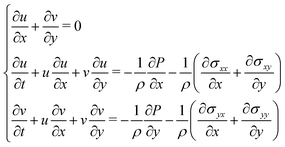 | (9) |
Based on different constitutive equations for the stress tensor appeared in eqn (9), various systems of PDEs are obtained to model complex fluids based on the type of material at hand. Even for a simple non-Newtonian fluid expressing PL behavior, the equation of motion becomes challenging to solve. There are several solvers for GNF models available; however, employing these solvers is far from trivial for modeling non-Newtonian flows for different geometries, and requires close familiarity with the software package. Moreover, the accuracy required to fully capture the detailed behavior of a complex fluid in various conditions will not be obtained due to the limitations of traditional numerical solvers. Here, we are leveraging the recent advancements in machine learning to solve the fluid flow behavior of complex fluids, regardless of the complexity of the model at hand. To this aim, we include a combination of eqn (9) and the rheological equations describing a complex fluid to the NN, and aim to predict the flow in a spatiotemporal domain.
2.3 Flow protocols
In this work, we chose various flow protocols and parameters to show the independence of our proposed method to any specifications on the type of flow. In order to prevent duplication and to have a reference for all future results, we summarize the flow protocols applied here in Fig. 1. We study the velocity profiles for a range of different constitutive models upon imposing a series of flow protocols, including pressure flows, boundary driven flows, strain imposed and stress imposed flows and oscillatory flow protocols, based on their relevance to rheological interrogation of complex fluids.
 |
| | Fig. 1 Schematic summary of the applied flow protocols in this study and their corresponding kinematics. These flow protocols are chosen due to their applicability and commonalities in rheological analysis of different non-Newtonian fluids. | |
2.4 Physics-informed neural networks
ML frameworks can be categorized in two different approaches based on the data at hand: supervised learning or unsupervised learning.68 Neural Networks are a subset of supervised ML algorithms, which correlate the complex relations between the inputs and outputs by creating a computational data-driven framework. This task is achieved by optimizing the neurons' variables to minimize the discrepancy between the predicted and the actual data. The traditional NN's training process is solely based on statistics, meaning that the NNs generate meta-models based on correlations in statistical variations of different complex systems. Hence, any prediction from these networks is naturally agnostic to the physical laws. Here, we are directly injecting the nonlinear physical governing laws without any prior assumptions such as linearization or local time-stepping to the NN architecture. We include the physical intuitions explicitly into the NN framework by leveraging the recent developments in Automatic Differentiation (AD)69 to differentiate the NN with respect to its input coordinates and model parameters. Fig. 2 shows a schematic description of nn-PINN. The input parameters are temporal (t) and spatial coordinates (x), and outputs are velocity (v) and shear stress (σ). In a thixotropic fluid, the number of outputs can be adjusted to capture the structure parameter as well. The outputs of this network are then utilized to calculate the loss function based on the physical law, initial conditions, and boundary conditions.
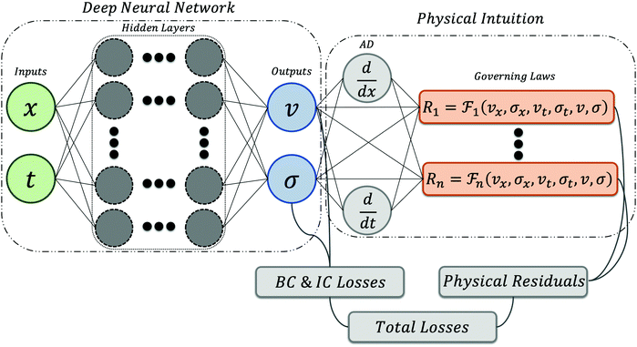 |
| | Fig. 2 Schematic illustrating the architecture of a non-Newtonian physics-informed neural network, which consists of two main parts: a Deep Neural Network (DNN) associated with the data (left part), and the correlation providing the association with the physical laws (right part). In the DNN part, the input layer (shown in green) consists of a spatial coordinate as x as well as temporal coordinate as t. For visual purposes, the output layer (shown in blue) contains only two outputs as velocity (v) and shear stress (σ). The layers that correlate inputs to outputs are hidden layers (shown in dark grey) and contain several neurons. Automatic Differentiation (AD) is employed to differentiate the output of the DNN with respect to the inputs. Subsequently, the physical governing laws (shown in brown) are introduced to guide the training process. As a motivating example, for a PL constitutive model as described in eqn (1) included in the network, the definitions of fi(![[thin space (1/6-em)]](https://www.rsc.org/images/entities/char_2009.gif) ) can be written as f1 = σ − μ0 ) can be written as f1 = σ − μ0![[small gamma, Greek, dot above]](https://www.rsc.org/images/entities/i_char_e0a2.gif) n and n and  . The boundary condition (BC) and initial condition (IC) losses are calculated based on the discrepancy between the predicted and actual value in the boundaries (for BC losses) and at the initial part of the process (for IC losses). . The boundary condition (BC) and initial condition (IC) losses are calculated based on the discrepancy between the predicted and actual value in the boundaries (for BC losses) and at the initial part of the process (for IC losses). | |
We define fi(x, y, t) to be given by the residuals of the system of PDE equations described in eqn (9) as well as stress tensor definitions, all in eqn (10).
| |  | (10) |
The traditional Neural Network algorithms are trained by the “training data”, and being tested by the “testing data”. However, in our proposed nn-PINN platform, instead of using data to train our network, we are using physical equations to guide the training process. Hence, we do not have a training data/testing data like the traditional data-based neural networks. In other words, during the training process, the variables of nn-PINN are learned by minimizing the loss function, a combination of each equation's residual, in addition to the discrepancy between the predicted and the actual ICs and BCs, described in
eqn (11).
| | | MSE = MSER + ω2MSEICs + ω3MSEBCs. | (11) |
In our system in
eqn (11), MSE
BC and MSE
IC are the discrepancies between the actual and the predicted values of the boundary conditions and initial conditions, respectively. MSE
R is the residual calculated from the system of PDEs. The mathematical definition of these parameters is provided in
eqn (12)–(14).
| |  | (12) |
| |  | (13) |
| |  | (14) |
In this study, instead of simply summing the residuals from BC, IC, and the system of PDEs, these losses are added based on some weight functions. In other words,
ωi is the contribution of different sources of residual. The main reason for using these weights is to enable control of the BCs/ICs effects. For instance, in cases with a slip BC, the weight of BC losses can be dialed down, so that the slip length/velocity in a certain domain can be recovered. For this study, since BCs and ICs are well-defined, one will need to find the best numbers for weights of each part of the loss function. To this aim, a comprehensive study of the role of these weights on the accuracy of the nn-PINN based on L2 norm defined in
eqn (15) is performed (
Table 1).
| |  | (15) |
It should be noted that all calculations presented here were carried out based on a Carreu–Yasuda fluid for a start-up of a flow.
Table 2 shows the L2-norm of nn-PINN architectures for different weights. In this study, the weights of BCs and ICs are chosen to be 20 and 50, respectively.
Table 1 The L2-norm (×10−3) based on different loss definitions based on their weights for a CY fluid in a start-up of a flow
|
ω
3
|
ω
2
|
| 1 |
10 |
20 |
50 |
| 1 |
5.63 |
6.25 |
5.72 |
5.59 |
| 10 |
4.78 |
3.21 |
3.45 |
4.49 |
| 20 |
6.29 |
3.77 |
3.54 |
3.89 |
| 50 |
7.91 |
3.76 |
3.18 |
4.72 |
Table 2 Errors in the L2 norm for different NN architectures based on their number of hidden layers (depth) and neurons per layer (width) on a single sample, keeping all other variables constant
| Width |
Depth |
| 1 |
2 |
4 |
8 |
| 10 |
0.169 |
0.0642 |
0.0346 |
0.0152 |
| 20 |
0.119 |
0.0444 |
0.0263 |
0.0109 |
| 50 |
0.107 |
0.0231 |
0.00318 |
0.0111 |
| 100 |
0.0966 |
0.0222 |
0.00833 |
0.00774 |
The design of NNs is a significant feature that needs to be extensively studied. The number of layers in a NN architecture as well as the number of neurons per layer can have an effect on the accuracy of NNs. Hence, the L2 norm as the measure of accuracy is employed to compare the role of the depth (number of hidden layers) and width (the number of neurons per layer) of the NN in the nn-PINN framework. This is used based on a predictive nn-PINN for a GNF (PL as the working model) in a start-up of a flow with top boundary condition of utop = 1 [m s−1] to eliminate any system-specific biases. As the width and depth of the system increases, the NN becomes more complex and the accuracy of the predictions changes. Nonetheless, this increase of complexity is not always necessarily in favor of enhancing the accuracy of the predictions. Often, adding more neurons to the NN can lead to overfitting, which in turn reduces the efficiency of the algorithm. Table 2 shows the L2 norm of different NN architectures in predicting the spatiotemporal flow based on a PL model. The architecture of the nn-PINN framework in this study is constructed by four hidden layers with 50 neurons in each layer, which is found to yield the best levels of accuracy to avoid overfitting.
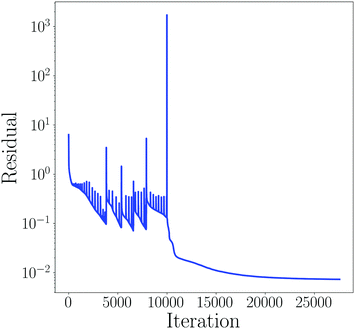
It should be noted that the loss function is optimized using a combination of Adams optimizer and LBFG-S method together with Xavier's initialization method, while the hyperbolic tangent function is employed as the activation function throughout this work. The convergence plot and residual losses for the nn-PINN architecture are shown in this section. The residual losses of the nn-PINN training phase are shown in Fig. 3. As inferred from the results, we only require ∼20![[thin space (1/6-em)]](https://www.rsc.org/images/entities/char_2009.gif) 000–25
000–25![[thin space (1/6-em)]](https://www.rsc.org/images/entities/char_2009.gif) 000 iterations to reach a properly trained metamodel that is deemed ready to be used for predictions. It should be noted that the criteria used throughout this study for the weighted total residual is to be less than 0.005.
000 iterations to reach a properly trained metamodel that is deemed ready to be used for predictions. It should be noted that the criteria used throughout this study for the weighted total residual is to be less than 0.005.
 |
| | Fig. 3 Required iterations during optimization of the loss function in the training process of nn-PINN. The sudden drop in the loss is caused by switching from the Adam to the L-BFGS optimizer. | |
All of the training and validations were completed on a computer with 32GB of RAM and an i7 processor. The longest training run time was two hours, with each training lasting an average of one hour. This means that only with a few hours of proper training, one can employ the trained nn-PINN to predict the spatiotemporal domain of a non-Newtonian fluid. It is worth mentioning that after training is done, the predictions can be made virtually instantaneously.
3 Results and discussion
Our main goal is to present a well-established, reliable, and accurate framework based on a physics-based ML algorithm in order to solve fluid flow problems containing non-Newtonian fluids. In other words, the NN is employed to find the solution to a rheologically relevant constitutive model in a given spatiotemporal domain with certain initial and boundary conditions. Thus, we present the predictions made using our nn-PINN framework for the non-Newtonian fluids following different GNF constitutive equations in various types of flow protocols of rheometric significance. Subsequently, we investigate the applicability of our proposed methodology to predict the behavior of the fluid with respect to more complex constitutive equations, namely viscoelastic and thixotropic phenomenological models. It should be noted that the highest Reynolds number throughout this paper is of O(10), and thus small enough to ignore any inertial effect.
3.1 Generalized Newtonian fluid
In the first step, we implement a series of GNF constitutive models into our nn-PINN platform and employ it as a data-driven tool to solve systems of coupled PDEs. It should be mentioned that this method uses the equations without any discretization and is completely based on training and consequent predictions, where the system of PDEs as well as the boundary and initial conditions are the only information used in the training process. Hence, the output of the nn-PINN will be the spatiotemporal response of the non-Newtonian fluid.
Before further testing of any data-driven approach, it is essential to demonstrate that the choice of model parameter has no effect on the predictions made by the metamodel. To do this, we adapted a simple power-law model (outlined in eqn (1) as the main constitutive model for the shear stress response of the fluid with three different power indices to enable comparison between different fluids: shear thinning (n = 0.8), Newtonian (n = 1.0), and shear thickening (n = 1.2). Fig. 4 presents the predicted spatiotemporal domain of a start-up flow protocol versus the numerical ground truth solution. We see from the results in the right hand panel for the error color maps, and from visual inspection of the nn-PINN predictions against the actual numerical solution, that our NN consistently predicts an accurate velocity profile for the fluid subject to the imposed strain, regardless of the power index, i.e. the nature of fluid. From the top row to the bottom row, the power index grows and the fluid nature transitions from shear-thinning to Newtonian, and to shear-thickening. As this transition occurs, the velocity profiles change systematically; however, the data-driven metamodel accurately tracks these changes with less than maximum of 4 percent error in all cases.
 |
| | Fig. 4 Velocity profiles for a power-law fluid in the spatiotemporal domain presented with no-slip boundary conditions at the walls and zero velocity initial conditions. The power law parameters for these results are ρ = 100 [kg m−3] and μ0 = 1 [Pa s]. The value of the shear rate exponent for the first to third rows is 0.8, 1.0, and 1.2, respectively. The first column panels are the actual numerical solution of the constitutive model in the domain, and the second column panels are the nn-PINN predictions. Third column panels represent the discrepancy between the nn-PINN predictions and the actual solutions. The coordinate across the velocity gradient (y-axis) is normalized by the size of the domain, and the color bars represent the velocity scales. | |
In the next step, we consider different (and most commonly used) GNF models outlined in eqn (1), (2), and (4) in a start-up of flow protocol, and compare the nn-PINN predictions against the numerical solutions. Fig. 5 shows the comparison between the ground truth solution of different GNF models and nn-PINN predictions in a start-up of shear flow protocol with a top boundary condition of Vtop = 1 [m s−1] while the bottom boundary is at rest. We expect a transient phase after applying the flow followed by a steady state upon reaching the linear velocity distribution. The parameters of each model are listed in Table 3.
 |
| | Fig. 5 Velocity profiles for GNF fluids in the spatiotemporal domain presented with no-slip boundary conditions at the walls and zero velocity initial conditions. Power-law, Herschel–Bulkly and Carreau–Yasuda GNF models are presented in the first, second and third row respectively. Model parameters are set based on Table 3. The first column panels are the actual numerical solution of the constitutive model in the domain, and the second column panels are the nn-PINN predictions. Third column panels represent the discrepancy between the nn-PINN predictions and the actual solutions. The coordinate across the velocity gradient (y-axis) is normalized by the size of the domain, and the color bars represent the velocity scales. | |
Table 3 The parameters of the GNF model for start-up of a flow shown in Fig. 4
| Model |
ρ [kg m−3] |
n
|
η [Pa s] |
η
0 [Pa s] |
η
∞ [Pa s] |
a
|
λ
|
σ
y
[Pa] |
| PL |
100 |
2 |
1 |
— |
— |
— |
— |
— |
| HB |
100 |
1.5 |
1 |
— |
— |
— |
— |
10 |
| CY |
100 |
0.5 |
— |
1 |
10 |
2 |
1.5 |
— |
On the third column of Fig. 5, we show the error in flow prediction using nn-PINN. The results in Fig. 5 clearly indicate that predictions of nn-PINN closely track the ground truth of the spatiotemporal response, regardless of the choice of model, since the local error in prediction is less than 2%. This is significant since models presented in Fig. 5 represent significantly different physical behaviors, and different mathematical complexities. For instance, the Herschel–Bulkly fluid uniquely mimics a yield-stress fluid and can be further extended to include shear-thinning effects as well.35,70 On the other hand, the Carreau–Yasuda model is very commonly used to describe the shear rheology of polymeric systems, having 2 terminal viscosities embedded in the model. As such, the results in Fig. 5 demonstrate that nn-PINN can be further generalized to include other GNF models of interest without losing accuracy and efficiency as well.
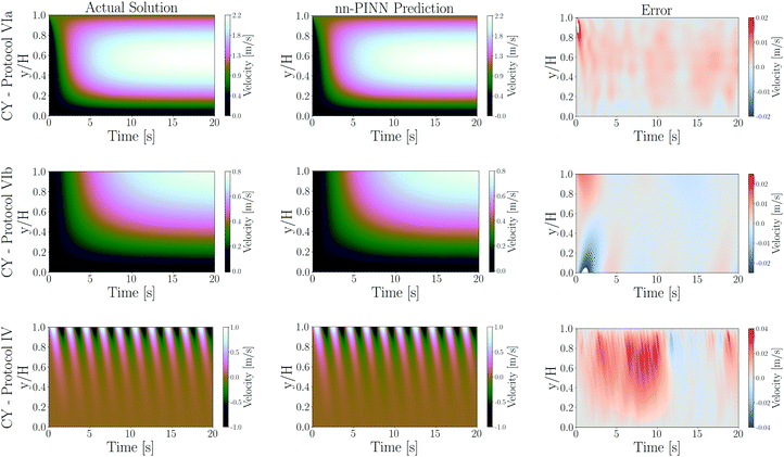
Having established the applicability and accuracy of nn-PINN with respect to the choice of GNF model and the model parameters, in the next step we seek to establish its applicability to different and more complex flow protocols. In practice, a number of different flow protocols can be applied to a non-Newtonian fluid to probe their properties and applicability. It is critical to ensure that the neural network provides a reliable prediction for all flow protocols as these experimentally relevant protocols are commonly encountered in various applications. To do so, we consider a Carreau–Yasuda fluid (as described in eqn (2)) in three flow protocols: a pressure–strain driven flow, a pressure–stress driven boundary, and a sinusoidal rate driven flow. The first two flow protocols become extremely important as one considers common processing methods such as extrusion or injection molding in which a combination of drag and pressure flows are present. In such geometries, it is essential to solve the constitutive equation for superposed flows to better design processing conditions. On the other hand, oscillatory flows are commonly used to probe rheological and viscoelastic properties of different fluids. It should be noted that the same analysis was performed for all different flow protocols with all of the GNF constitutive models as well, and for the sake of perspicuity only three of these cases are presented. However, the results and the accuracies remain consistent regardless of the choice of model here as well. Fig. 6 shows the comparison between the nn-PINN predictions and the ground numerical solutions of these flows for a Carreau–Yasuda model.
 |
| | Fig. 6 Velocity profiles for a Carreau–Yasuda fluid in the spatiotemporal domain presented with no-slip boundary conditions at the walls and zero velocity initial conditions. The model parameters are set to be ρ = 1000 [kg m−3], n = 0.8, μ0 = 3 [Pa s], μ∞ = 60 [Pa s], a = 2, λ = 3, and a = 2. The first column panels are the actual numerical solution of the constitutive model in the domain, and the second column panels are the nn-PINN predictions. The third column panels represent the discrepancy between the nn-PINN predictions and the actual solutions. The coordinate across the velocity gradient (y-axis) is normalized by the size of the domain, and the color bars represent the velocity scales. The first two rows represent the results under pressure and drag flows, and the final row presents oscillatory flow. | |
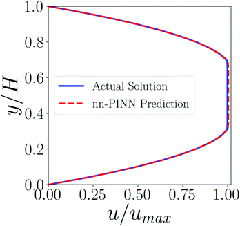
To further examine the differences in predicted flows by nn-PINN and the ground truth solution, steady-state velocity profiles of a Bingham fluid are compared in Fig. 7. As shown in the compared profiles, the nn-PINN is found to predict the yield point accurately. One should note that some commercial solvers commonly face challenges in solving for the yield point, and thus an alteration of the Bingham or the Herschel–Bulkly models with an arbitrarily large viscosity is used at a given threshold to avoid diverging zero shear viscosities. Nonetheless, nn-PINN directly uses the constitutive models as written with no further modification.
 |
| | Fig. 7 Predicted vs. calculated steady-state velocity profiles of a Bingham fluid in a Poiseuille flow with ρ = 500 [kg m−3], η = 0.1 [Pa], and σy = 1 [Pa]. | |
For all three complex flow protocols studied, the error panels in the right hand column suggest that nn-PINN deviates slightly from the numerical solution; these errors diminish after a few seconds of flow upon reaching a quasi-steady state. It should be mentioned that similar benchmarks with a wide range of boundary and initial conditions, model parameters, and flow protocols were performed, and the nn-PINN predictions were consistently found not to be limited by the choices made for any of the aforementioned parameters.
3.2 Viscoelastic fluids
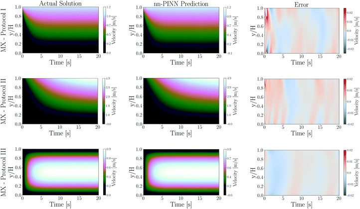
To capture the natural timescale of the material, phenomenological models have been developed in which the viscoelastic nature of the fluid under question is represented through distinct but connected elastic and fluid elements. These models generally involve using spring components for the elastic response of the material and dashpot components to mimic the viscous response under flow. These components can be connected in series (leading to the Maxwell equation) or in parallel (leading to the Kelvin model). Here, we adopt a Maxwell fluid as shown in eqn 5 in three different flow protocols as strain imposed, stress imposed, and pressure driven flows. The velocity and stress contours are shown in Fig. 8 and 9, respectively. In the stress response of the fluid in a strain imposed flow protocol, there is a gradient in the beginning of the flow, which is diminished after some time by reaching a steady state value. On the other hand, in the stress imposed flow protocol, the imposed stress is propagating to the fluid over time until it reaches the bottom boundary and after that the entire domain is experiencing a steady state value for stress, which is the same as the imposed stress. In the pressure driven flow, there is a symmetry in the value of the stress with a sign change in the center-line.
 |
| | Fig. 8 Velocity profiled across the spatiotemporal domain for a Maxwell fluid in various flow protocols. The model parameters are set to be ρ = 30 [kg m−3], G = 100 [Pa], and η = 2 [Pa s]. The first column is the actual solutions, the second column is the nn-PINN predictions, and the last column is the discrepancy between the predictions and actual solutions. The first row shows strain imposed flow, second row panels correspond to stress imposed flow and the last row represents pressure driven flow. | |
 |
| | Fig. 9 Shear stress response across the spatiotemporal domain for a Maxwell fluid in various flow protocols. The model parameters are set to be ρ = 30 [kg m−3], G = 100 [Pa], and η = 2 [Pa s]. The first column is the actual solutions, the second column is the nn-PINN predictions, and the last column is the discrepancy between the predictions and actual solutions. The first row shows strain imposed flow, second row panels correspond to stress imposed flow and the last row represents pressure driven flow. | |
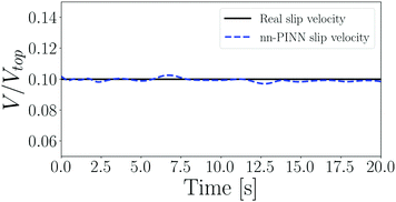
To address a common experimental artifact in rheologically relevant flows and perform another test of the model efficiency with different boundary conditions, we also investigated the applicability of nn-PINN in predicting the slip boundary condition. Slip parameter as ε = ubottom/utop is defined, and by changing this parameter we are able to acquire different levels of slippage. As a motivating example, we considered a Maxwell fluid with three cases as ε = 0.01, ε = 0.05, and ε = 0.10 leading to three different levels of slip velocities of: 1%, 5%, and 10% of the maximum velocity at the upper boundary. In either case, we assume that the bottom boundary has a slip velocity proportional to the applied shear rate to the top boundary. The results for the slip boundary condition are shown in Fig. 10. The results in Fig. 10 clearly indicate that the nn-PINN model can also recover the numerical solution at the boundaries with different wall slip conditions without losing accuracy. Considering the fact that PINNs have been proven very effective for inverse problems, these models can be used in quantifying the wall-slip and similar experimental artifacts effectively. To test this, we considered a case in which the bottom boundary condition is associated with 10% wall-slip as an unknown to the nn-PINN. The goal is to determine the functionality of the slippage velocity at the boundary, based on existing velocity profiles. To do so, we assume a handful of sparse data of the flow field is available. To be more precise, we consider some velocity sensors placed randomly in the spatiotemporal domain. In order to determine the unknown slippage boundary condition, we also added eqn (16) to the total loss function defined in eqn (11) with a weight of ω3.
| |  | (16) |
In addition, a side neural network is assigned to track and predict the unknown boundary velocity.
Fig. 11 represents the predicted velocity at the bottom boundary. In addition, we are able to find the stress field in the entire spatiotemporal domain with a great accuracy. This suggests that even with an ill-posed problem, only having a handful of data (∼50), nn-PINN enables a full reconstruction of the entire spatiotemporal velocity as well as the stress contours in the geometry under question.
 |
| | Fig. 10 Velocity profiled for a Maxwell fluid in spatiotemporal domain with included wall slip at three different levels of 1%, 5%, and 10%, in the first, second and third rows respectively. The model parameters are set to be ρ = 30 [kg m−3], G = 100 [Pa], and η = 2 [Pa s]. The first column is the actual solutions, the second column is the nn-PINN predictions, and the last column is the discrepancy between the predictions and actual solutions. | |
 |
| | Fig. 11 Predicted velocity at the bottom boundary condition with slippage. | |
3.3 Thixtropic fluids
To fully probe the capability of our proposed methodology in predicting the spatiotemporal response of a non-Newtonian fluid, we also implemented a TEVP fluid following eqn (6). Fig. 12 represents the comparison between the nn-PINN predictions and the ground solutions of the Thixotropic fluid for start-up of flow with three different initial conditions as fully structurized, fully fluidized, and half structurized fluid. A constant velocity of Vtop = 1 [m s−1] is applied on the top boundary while the bottom one is at rest. The contour panels show the results for the velocity profiles across the velocity gradient direction as a function of time, as well as the structure parameter, λ, at the same coordinates to show the correlation between fluidization processes and the resulting flow kinematics. As it can be seen from the error contours in the right hand side column of Fig. 12, nn-PINN gives a robust set of predictions with virtually no deviation from the ground solution of the constitutive equation, regardless of the structure parameter choice at the outset. Results in Fig. 12 further demonstrate the ability of these data-driven models to recover the fully resolved numerical solution of complex fluids with several material and flow timescales involved.
 |
| | Fig. 12 Velocity profiles (first, third, and fifth rows) and structure parameter (second, fourth, and sixth rows) prediction in the spatiotemporal domain for a TEVP fluid under start-up of shear flow protocol. The model parameters are set to be ρ = 30 [kg m−3], G = 100 [Pa], ηs = 5 [Pa s], ηp = 1 [Pa s], k+ = 0.1, and k− = 0.3. The first column is the actual solutions, the second column is the nn-PINN predictions, and the last column is the discrepancy between the predictions and actual solutions. | |
4 Conclusions
In this work, we presented a data-driven algorithm, nn-PINN, and comprehensively studied the performance of the proposed method for modeling the spatiotemporal behavior of a variety of complex fluids with different non-Newtonian constitutive models. The nn-PINN methodology leverages the recent advances and ever-increasing benefits of NNs in solving complex systems of coupled PDEs, allowing us to develop an alternative method for solving constitutive models for complex fluids in conjunction with the conservation of momentum and mass equations. This is particularly of interest with respect to complex rheological constitutive models that are challenging to implement within CFD solvers of choice. Commonly used flow protocols in the rheometry of complex fluids were examined, for different constitutive models of choice from simple generalized Newtonian, to thixotropic elaso-visco-plastic. The transient and steady state velocity profiles of the flow with these variations are presented to establish the applicability of the nn-PINN in handling different types of governing equations. The method was consistently found to recover the fully resolved numerical solution of the flow kinematics under the same spatiotemporal domain. We also systematically interrogated the applicability and adaptability of nn-PINN to the initial and boundary conditions and material/model parameters. Our study of the unknown boundary conditions in an inverse problem suggests that nn-PINNs can be employed to solve for a full reconstruction of velocity and stress fields having a few data points across the entire domain. These detailed investigations demonstrate clearly that the proposed model can rigorously track the ground truth solution of the constitutive equations, regardless of the choice of model, its parameters, and initial/boundary conditions. Needless to mention that benchmarking and detailed testing of the model have been performed on an exhaustive list of boundary conditions, initial conditions, noise levels, other constitutive models, and flow protocols; nonetheless, and for the sake of brevity a number of motivating examples have been selected for presentation here.
Our findings strongly suggest that data-driven models informed by the physical processes can make a leap in flow simulations of complex fluids. Investigation of complex geometries/domains, other tensorial descriptions of complex fluids, and most importantly the inverse solution of models based on data will be of particular interest and of great practical importance. For instance, three dimensional flows in which shear-banding and vorticity-banding occur, or complex contracting/diverging geometries are of great relevance to many real-world flows of interest.
Conflicts of interest
The authors declare that there is no conflict of interest.
Acknowledgements
M. M. and S. J. would like to acknowledge support by Northeastern University's Spark Fund program. G. K. was supported by DOE PhILMS Grant No. DE-SC0019453.
Notes and references
-
F. A. Morrison, Understanding Rheology, Oxford University Press, 2001 Search PubMed.
-
C. W. Macosko, Rheology: principles, measurements, and applications, VCH, 1994 Search PubMed.
-
R. B. Bird, R. C. Armstrong and O. Hassager, Dynamics of Polymeric Liquids: Fluid mechanics, Wiley, 1987 Search PubMed.
-
J. Mewis and N. J. Wagner, Colloidal Suspension Rheology, Cambridge University Press, Cambridge, 2011 Search PubMed.
- P. R. de Souza Mendes, Soft Matter, 2011, 7, 2471 RSC.
- A. K. Gurnon and N. J. Wagner, J. Fluid Mech., 2015, 769, 242–276 CrossRef CAS.
- S. A. Rogers, D. Vlassopoulos and P. T. Callaghan, Phys. Rev. Lett., 2008, 100, 128304 CrossRef CAS.
- C. J. Dimitriou and G. H. McKinley, Soft Matter, 2014, 10, 6619–6644 RSC.
- W. M. Gelbart and A. Ben-Shaul, J. Phys. Chem., 1996, 100, 13169–13189 CrossRef CAS.
- J. Vermant and M. J. Solomon, J. Phys.: Condens. Matter, 2005, 17, R187–R216 CrossRef CAS.
- K. Masschaele, J. Fransaer and J. Vermant, Soft Matter, 2011, 7, 7717–7726 RSC.
- N. J. Wagner and J. F. Brady, Phys. Today, 2009, 62, 27–32 CrossRef CAS.
- R. H. Ewoldt, A. E. Hosoi and G. H. McKinley, J. Rheol., 2008, 52, 1427–1458 CrossRef CAS.
- R. H. Ewoldt and G. H. McKinley, Rheol. Acta, 2017, 56, 195–210 CrossRef CAS.
- K. Hyun, M. Wilhelm, C. O. Klein, K. S. Cho, J. G. Nam, K. H. Ahn, S. J. Lee, R. H. Ewoldt and G. H. McKinley, Prog. Polym. Sci., 2011, 36, 1697–1753 CrossRef CAS.
- R. G. Larson, J. Rheol., 2015, 59, 595–611 CrossRef CAS.
- R. G. Larson and Y. Wei, J. Rheol., 2019, 63, 477–501 CrossRef CAS.
- S. Jamali, R. C. Armstrong and G. H. McKinley, Mater. Today Adv., 2020, 5, 100026 CrossRef.
- T. Divoux, V. Grenard and S. Manneville, Phys. Rev. Lett., 2013, 110, 018304 CrossRef.
- S. Jamali, R. C. Armstrong and G. H. McKinley, Phys. Rev. Lett., 2019, 123, 248003 CrossRef PubMed.
- Y. Wei, M. J. Solomon and R. G. Larson, J. Rheol., 2018, 62, 321–342 CrossRef CAS.
- P. R. de Souza Mendes and R. L. Thompson, J. Non-Newtonian Fluid Mech., 2012, 187–188, 8–15 CrossRef CAS.
- R. Radhakrishnan, T. Divoux, S. Manneville and S. M. Fielding, Soft Matter, 2017, 13, 1834–1852 RSC.
- S. Jamali, G. H. McKinley and R. C. Armstrong, Phys. Rev. Lett., 2017, 118, 048003 CrossRef PubMed.
- M. Geri, R. Venkatesan, K. Sambath and G. H. McKinley, J. Rheol., 2017, 61, 427–454 CrossRef CAS.
-
N. Phan-Thien and N. Mai-Duy, Understanding Viscoelasticity, Springer International Publishing, Cham, 2017 Search PubMed.
-
J. H. Ferziger and M. Peric, Computational Methods for Fluid Dynamics, Springer Berlin Heidelberg, 2012 Search PubMed.
-
D. R. Durran, Numerical Methods for Fluid Dynamics: With Applications to Geophysics, Springer, New York, 2010 Search PubMed.
-
M. Holt, Numerical Methods in Fluid Dynamics, Springer Berlin Heidelberg, 2012 Search PubMed.
- M. H. Zawawi, A. Saleha, A. Salwa, N. H. Hassan, N. M. Zahari, M. Z. Ramli and Z. C. Muda, AIP Conf. Proc., 2018, 020252 CrossRef.
- P. Kieckhefen, S. Pietsch, M. Dosta and S. Heinrich, Ann. Rev. Chem. Biomol. Eng., 2020, 11, 397–422 CrossRef CAS PubMed.
- D. Kochkov, J. A. Smith, A. Alieva, Q. Wang, M. P. Brenner and S. Hoyer, Proc. Natl. Acad. Sci. U. S. A., 2021, 118, e2101784118 CrossRef CAS PubMed.
-
O. Obiols-Sales, A. Vishnu, N. Malaya and A. Chandramowliswharan, Proceedings of the 34th ACM International Conference on Supercomputing, New York, NY, USA, 2020, pp. 1–12 Search PubMed.
- H. Zhong, Q. Xiong, L. Yin, J. Zhang, Y. Zhu, S. Liang, B. Niu and X. Zhang, Renewable Energy, 2020, 152, 613–626 CrossRef CAS.
- M. Mahmoudabadbozchelou, M. Caggioni, S. Shahsavari, W. H. Hartt, G. Em Karniadakis and S. Jamali, J. Rheol., 2021, 65, 179–198 CrossRef CAS.
- K. A. Janes and M. B. Yaffe, Nat. Rev. Mol. Cell Biol., 2006, 7, 820–828 CrossRef CAS PubMed.
- D. P. Solomatine and A. Ostfeld, J. Hydroinformatics, 2008, 10, 3–22 CrossRef.
-
D. Solomatine, L. M. See and R. Abrahart, Practical hydroinformatics, 2009, pp. 17–30 Search PubMed.
- H. Lei, L. Wu and W. E, Phys. Rev. E, 2020, 102, 043309 CrossRef CAS PubMed.
- R. Ershadnia, M. A. Amooie, R. Shams, S. Hajirezaie, Y. Liu, S. Jamshidi and M. R. Soltanian, J. Petrol. Sci. Eng., 2020, 185, 106641 CrossRef CAS.
- M. Mahmoudabadbozchelou and S. Jamali, Sci. Rep., 2021, 11, 12015 CrossRef CAS PubMed.
- M. Raissi, P. Perdikaris and G. E. Karniadakis, J. Comput. Phys., 2019, 378, 686–707 CrossRef.
- X. Jin, S. Cai, H. Li and G. E. Karniadakis, J. Comput. Phys., 2021, 426, 109951 CrossRef.
- Z. Mao, A. D. Jagtap and G. E. Karniadakis, Comput. Methods Appl. Mech. Eng., 2020, 360, 112789 CrossRef.
-
S. Cai, Z. Wang, C. Chryssostomidis and G. E. Karniadakis, Volume 3: Computational Fluid Dynamics; Micro and Nano Fluid Dynamics, 2020 Search PubMed.
- S. Cai, Z. Wang, S. Wang, P. Perdikaris and G. E. Karniadakis, J. Heat Transfer, 2021, 143, 060801 CrossRef CAS.
- A. D. Jagtap and G. E. Karniadakis, Commun. Comput. Phys., 2020, 28, 2002–2041 CrossRef.
- X. Meng, Z. Li, D. Zhang and G. E. Karniadakis, Comput. Methods Appl. Mech. Eng., 2020, 370, 113250 CrossRef.
- G. Pang, L. Lu and G. E. Karniadakis, SIAM J. Sci. Comput., 2018, 41, A2603–A2626 CrossRef.
-
G. Pang, M. D'Elia, M. Parks and G. E. Karniadakis, 2020, arXiv:2004.04276.
- H. Jiang, Z. Nie, R. Yeo, A. B. Farimani and L. B. Kara, J. Appl. Mech., 2021, 88, 051005 CrossRef.
- K. Meidani and A. Barati Farimani, Comput. Methods Appl. Mech. Eng., 2021, 381, 113831 CrossRef.
- P. Pant, R. Doshi, P. Bahl and A. B. Farimani, Phys. Fluids, 2021, 33, 107101 CrossRef CAS.
- K. Xu and E. Darve, Comput. Methods Appl. Mech. Eng., 2021, 384, 113976 CrossRef.
- K. Xu, D. Z. Huang and E. Darve, J. Comput. Phys., 2021, 428, 110072 CrossRef.
- P. Coussot, J. Non-Newtonian Fluid Mech., 2014, 211, 31–49 CrossRef CAS.
- D. Bonn, M. M. Denn, L. Berthier, T. Divoux and S. Manneville, Rev. Mod. Phys., 2017, 89, 35005 CrossRef.
- E. C. Bingham, Bull. Bur. Stand., 1916, 13, 309 CrossRef.
- J.-Y. Kim, J.-Y. Song, E.-J. Lee and S.-K. Park, Colloid Polym. Sci., 2003, 281, 614–623 CrossRef CAS.
- I. Kaneda and A. Sogabe, Colloids Surf., A, 2005, 270, 163–170 CrossRef.
- G. Petekidis, D. Vlassopoulos and P. Pusey, J. Phys.: Condens. Matter, 2004, 16, S3955 CrossRef CAS.
- N. Koumakis, A. Pamvouxoglou, A. S. Poulos and G. Petekidis, Soft Matter, 2012, 8, 4271–4284 RSC.
- C. Pellet and M. Cloitre, Soft Matter, 2016, 12, 3710–3720 RSC.
- W. H. Herschel and R. Bulkley, Kolloid-Z., 1926, 39, 291–300 CrossRef.
- J. Mewis, J. Non-Newtonian Fluid Mech., 1979, 6, 1–20 CrossRef CAS.
- H. A. Barnes, J. Non-Newtonian Fluid Mech., 1997, 70, 1–33 CrossRef CAS.
- A. Mujumdar, A. N. Beris and A. B. Metzner, J. Non-Newtonian Fluid Mech., 2002, 102, 157–178 CrossRef CAS.
- S. L. Brunton, B. R. Noack and P. Koumoutsakos, Annu. Rev. Fluid Mech., 2020, 52, 477–508 CrossRef.
-
A. G. Baydin, B. A. Pearlmutter, A. A. Radul and J. M. Siskind, 2015, arXiv:1502.05767.
- M. Caggioni, V. Trappe and P. T. Spicer, J. Rheol., 2020, 64, 413–422 CrossRef CAS.
|
| This journal is © The Royal Society of Chemistry 2022 |
Click here to see how this site uses Cookies. View our privacy policy here.  a,
George Em.
Karniadakis
b and
Safa
Jamali
 *a
*a
![[small gamma, Greek, dot above]](https://www.rsc.org/images/entities/i_char_e0a2.gif) n
n
![[small gamma, Greek, dot above]](https://www.rsc.org/images/entities/i_char_e0a2.gif)
![[small gamma, Greek, dot above]](https://www.rsc.org/images/entities/i_char_e0a2.gif) n
n
![[small gamma, Greek, dot above]](https://www.rsc.org/images/entities/i_char_e0a2.gif) is the shear rate, and k+ and k− are system-specific build-up and breakage time constants for the time-evolution of the structure parameter. As the TEVP model brings together viscoelastic and plastic components, ηp represents the viscosity that emerges from the particulate phase's structure under flow, and as such can be considered a plastic viscosity.
is the shear rate, and k+ and k− are system-specific build-up and breakage time constants for the time-evolution of the structure parameter. As the TEVP model brings together viscoelastic and plastic components, ηp represents the viscosity that emerges from the particulate phase's structure under flow, and as such can be considered a plastic viscosity.
![[v with combining low line]](https://www.rsc.org/images/entities/i_char_0076_0332.gif) is the velocity vector, and σ is the stress tensor.
is the velocity vector, and σ is the stress tensor.

![[v with combining low line]](https://www.rsc.org/images/entities/i_char_0076_0332.gif) = (u, v) can be assumed for the fluid motion. Hence, the system of PDEs can be written as eqn (9):
= (u, v) can be assumed for the fluid motion. Hence, the system of PDEs can be written as eqn (9):

![[thin space (1/6-em)]](https://www.rsc.org/images/entities/char_2009.gif) ) can be written as f1 = σ − μ0
) can be written as f1 = σ − μ0![[small gamma, Greek, dot above]](https://www.rsc.org/images/entities/i_char_e0a2.gif) n and
n and  . The boundary condition (BC) and initial condition (IC) losses are calculated based on the discrepancy between the predicted and actual value in the boundaries (for BC losses) and at the initial part of the process (for IC losses).


![[thin space (1/6-em)]](https://www.rsc.org/images/entities/char_2009.gif) 000–25
000–25![[thin space (1/6-em)]](https://www.rsc.org/images/entities/char_2009.gif) 000 iterations to reach a properly trained metamodel that is deemed ready to be used for predictions. It should be noted that the criteria used throughout this study for the weighted total residual is to be less than 0.005.
000 iterations to reach a properly trained metamodel that is deemed ready to be used for predictions. It should be noted that the criteria used throughout this study for the weighted total residual is to be less than 0.005.