Ion accumulation-induced capacitance elevation in a microporous graphene-based supercapacitor

Abstract

High-performance porous 3D graphene-based supercapacitors are one of the most promising and challenging directions for future energy technologies. Microporous graphene has been synthesized by the pyrolysis method. The fabricated lightweight graphene with a few layers (FLG) has an ultra-high surface area of 2266 m² g⁻¹ along with various-sized micropores. The defect-induced morphology and pore size distribution of the fabricated graphene are examined, and the results show that the micropores vary from 0.85 to 1.9 nm and the 1.02 nm pores contribute 30% of the total surface area. The electrochemical behaviour of the electrode fabricated using this graphene has been studied with various concentrations of the KOH electrolyte. The highest specific capacitance of the graphene electrode of 540 F g⁻¹ (close to the theoretical value, ∼550 F g⁻¹) can be achieved by using the 1 M KOH electrolyte. This high specific capacitance contribution involves the counter ion adsorption, co-ion desorption, and ion permutation mechanisms. The formation of a Helmholtz layer, as well as the diffusion of the electrolyte ions, confirms this phenomenon. The symmetrical solid-state supercapacitor fabricated with the graphene electrodes and PVA–KOH gel as the electrolyte exhibits excellent energy and power densities of 18 W h kg⁻¹ and 10.2 kW kg⁻¹, respectively. This supercapacitor also shows a superior 100% coulombic efficiency after 6000 cycles.

---

1. Introduction

The ever-increasing human population has led to large energy consumption while fossil fuel energy sources simultaneously decrease.¹ To overcome these crises, renewable energy sources have become promising as they cover more than 30% of the energy requirement.² High power density, safe and environment-friendly energy storage systems must store their energy uninterruptedly.³ Among the various energy storage systems, supercapacitors are far superior to batteries in terms of their power density, long cycling life, and durability.^4–6

Supercapacitors that store energy electrostatically are known as an electric double-layer capacitors (EDLCs) and those based on faradaic reactions are known as pseudocapacitors.^5–7 Its light weight, large surface area (theoretically ∼2180 to ∼3100 m² g⁻¹), excellent conductivity, and fast charge–discharge phenomena, with a limited specific capacitance of ∼250 F g⁻¹, have enhanced the popularity of high surface area-based porous carbon for EDLCs.^3,5,8 Competing with various carbon-based materials, graphene exhibits a high theoretical specific capacitance of ∼550 F g⁻¹, with excellent conductivity, mechanical durability, high selectivity, and high surface area (∼2630 m² g⁻¹), but in practice, its experimental specific capacitances have been limited to ∼300 F g⁻¹.^4,8–10

Efforts have been made to achieve high specific capacitance in graphene-based supercapacitors, such as doping with various elements and forming composites with metal oxides or conducting polymers. 3D graphene foam is a carbon-based material that can improve the flexibility and number of pores for electron transport in comparison to 2D graphene sheets due to the reduction of agglomeration.^11,12 The porous carbon structure with adequate nanopores allows for numerous active sites and defects, which are preferable for charge accumulation, contributing to achieving high-performance supercapacitors.^3,13 Porous 3D graphene is considered an ‘electric sponge’ that can absorb electrolyte ions. Therefore, graphene with optimum pore sizes is favorable for making high-performance supercapacitors.^5,6

Various templates have been used to acquire nanopores in the carbon chain of graphene, which require acid etching of the templates and impurity removal, making it expensive and complicated.^3,9,14 In this regard, currently, blowing or copolymerization methods are widely used to achieve foam/nanosized pore architectures of functional materials due to their low cost, simpler operation, and large-scale production. This method is composed of three major steps. Initially, the precursors and blowing agents are mixed thoroughly. At the intermediate stage, the foam is formed by nucleation or external effort in which the blowing agent and the precursors pass through gas–liquid phases to form a soft fluid-like foam due to a chemical reaction. Finally, the desired product is stabilized by solidification or crystallization. The pyrolysis of organic precursors or decomposition of inorganic salts used in this study is an example of blowing away trapped gases to produce a porous structure.

Besides the electrodes, the electrolyte nature, such as the solution concentration and cation/anion size, plays a crucial role in the performance of supercapacitors. Carbon materials with suitable pore size distribution and high surface area are of research interest to improve the capacitance of electrodes, particularly those with a pore size less than 1 nm (i.e. less than the solvated ion size), by dissolving electrolyte ions in the subnanometer pores.^5,15 Therefore, several methods such as activation and carbonization have been adopted to develop porous materials. Based on the International Union of Pure and Applied Chemistry (IUPAC) classification, the nature of pores can be divided into three categories, namely macropores (>50 nm), mesopores (2–50 nm), and micropores (0.2–2 nm).¹⁶ Nanosized micropores can be subdivided into two types: ultra micropores (<0.7 nm) and supermicropores (>0.7 nm).¹⁶ In this study, we will concentrate on developing microporous graphene to provide a high-performance supercapacitor.

In this report, we prepare a porous graphene-based electrode material via the copolymerization method. A high surface area with uniformly distributed micropores with defects is obtained from the fabricated graphene electrodes. The electrodes exhibit high specific capacitance, equal to their theoretical value, using an optimized KOH electrolyte. Furthermore, we produce a solid-state supercapacitor based on the electrodes and analyze the capacitance contribution and charge storage mechanism.

2. Experimental

Porous graphene was fabricated by the decomposition reaction of a dextrose and NH₄Cl mixture in an argon atmosphere. The mixture was slowly heated (@4 °C min⁻¹) at 950 °C for 4.5 h. The solid dextrose was transformed into a fluid-like state above 150 °C, and the NH₄Cl decomposed into NH₃ and HCl gases at 350 °C. These gases slowly and steadily polymerized the fluid-like state to a thin bubble-walled polymer or soft fluid-like foam. After reaching ∼550 °C, this thin polymer was transformed into a graphitic layer via the carbonization process. At a temperature of 950 °C, the formed excessive gasses burst the graphitic layer to form a lightweight, high-surface area and porous graphene foam. The behaviour of the graphene made in this study and its supercapacitor will be shown and discussed in the following sections.

3. Results and discussion

3.1 Microstructural observation of the fabricated graphene

The porous nature of graphene foam was confirmed by field emission scanning electron microscopy (FESEM) and transmission electron microscopy (TEM). The FESEM images (Fig. 1a and b) reveal a sponge-like architecture composed of both open and closed pores. The closed vent foams are composed of pores separated by discrete gas release pockets, as shown in Fig. 1a, whereas individual graphene sheets are bent and randomly coiled without any agglomeration, and are damaged to form an open vent foam (Fig. S1a and b†). This porous graphene structure observed from FESEM consists of ∼1.6 μm average-sized pores including curved concave sheets with ripples (Fig. 1b and S1a, b†). All the graphene sheets have rugged surfaces with sizes varying from 7 to 11 μm. This type of structure is developed due to the corrugation of polymers at high temperature.¹⁷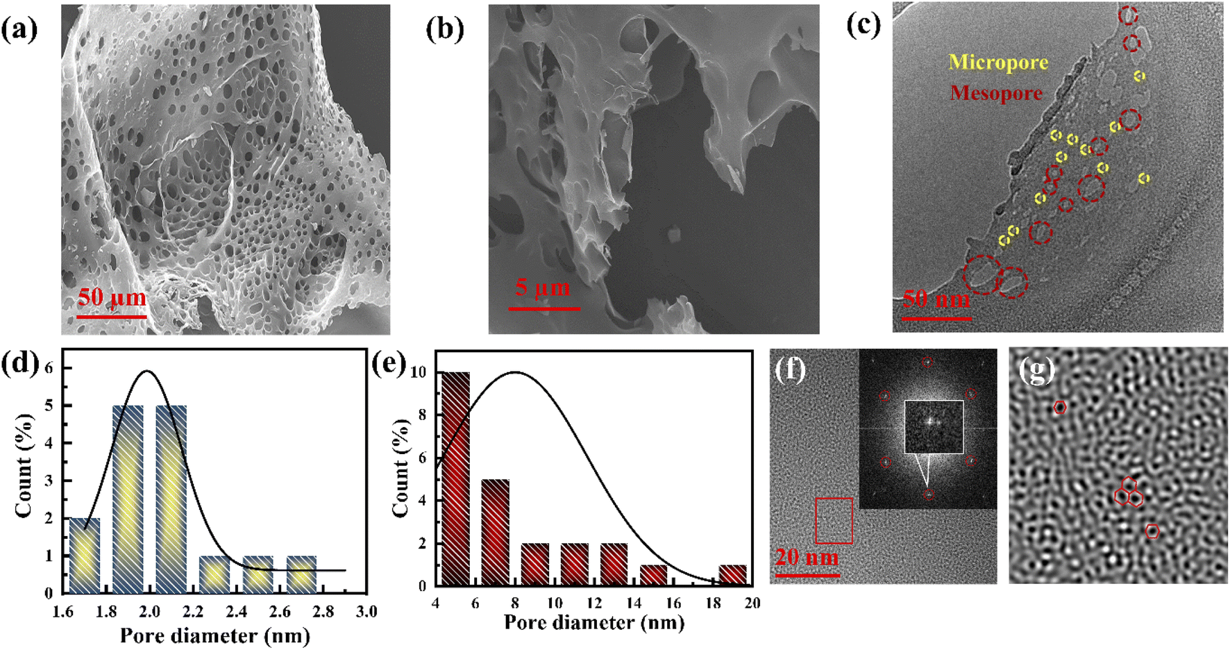

Fig. 1 (a and b) FESEM images of the porous graphene. (c) TEM image of the porous graphene (yellow circles highlight micropores and red circles highlight mesopores). (d and e) Statistical pore size distribution of the micropores and mesopores. (f) HRTEM images of the porous graphene layer. Inset shows the FFT of the porous graphene layer. (g) Filter image of the rectangular red-marked area in (f).

It is difficult to observe the micropores and mesopores from the above FESEM micrographs. However, such pores can be observed in the TEM images. The microstructure of sheet-type porous graphene (∼6 μm dimension) composed mainly of mesopores (average pore size of 9 nm) and surrounded by micropores (average pore size of 1.9 nm), according to Aboav–Weaire's and Lewis' law,¹⁸ was observed from the TEM images (Fig. 1c–e and S2a–c†). The graphene sheets show multiple hexagonal carbon architectures with atomic vacancy defects (Fig. 1f and g). A few concave-like circular graphene layers with an interplanar spacing of 0.39–0.43 nm are formed due to the eruptive species at high temperatures, confirming the presence of stacked multilayer graphene with surface defects (Fig. S2d–f†) rather than amorphous carbon.¹⁷ Few-layered graphene (FLG) with clear straight edges is also identified from the HRTEM images with a calculated interplanar distance of 0.37 nm, which reveals that typically 5–6 graphene layers are restacked, as shown in Fig. S2g and h.†

3.2 Structural study of the fabricated graphene

The presence of (002) peaks at 23.4° along with additional (100) and (101) peaks at 41.8° and 43.2°, respectively, in the X-ray diffraction (XRD) spectra confirms the well crystallized graphene layers (Fig. S3†).^19,20 Based on Lorentzian fitting, the (002) peak is the combination of several peaks with d spacings that vary from 3.42 to 4.16 Å, which confirms FLG (∼5) (Fig. S3† (inset)),²¹ corroborating the observation of the TEM micrographs (Fig. S2g and h†). The calculated crystallite width D (13.25 Å) and crystallite size L (68 Å) are similar to those of the graphene produced by the exfoliation of graphitic oxide.²² The slightly sharper intensities of those peaks (Fig. S3†) are attributed to defects, especially pores, which is consistent with the TEM results (Fig. 1g).

Fig. 2a presents the Raman spectra in the range of 1000 to 3000 cm⁻¹, to investigate the defects, the number of layers, and the porous nature of graphene.²³ Two overlapped broad peaks appear at 1325 cm⁻¹ (D band) and 1584 cm⁻¹ (G band), with a broad 2D band appearing at 2694 cm⁻¹, attributed to sp² bonded C–C chains and rings, defects, and the 2nd order zone boundary of phonons, respectively.^24–26 It has been well established that a high intensity of the D band indicates the presence of enormous defects at the edges and grain boundaries.^17,25 The five peaks are combined to create overlapped D and G bands (Fig. S4a†) attributed to the existence of the D′ (1604 cm⁻¹) band caused by defects.^22,25,27 Other peaks located at 1180 cm⁻¹ (D¹ band) and 1517 cm⁻¹ (D² band) are assigned to the sp² configuration and amorphous carbon, respectively.²⁸

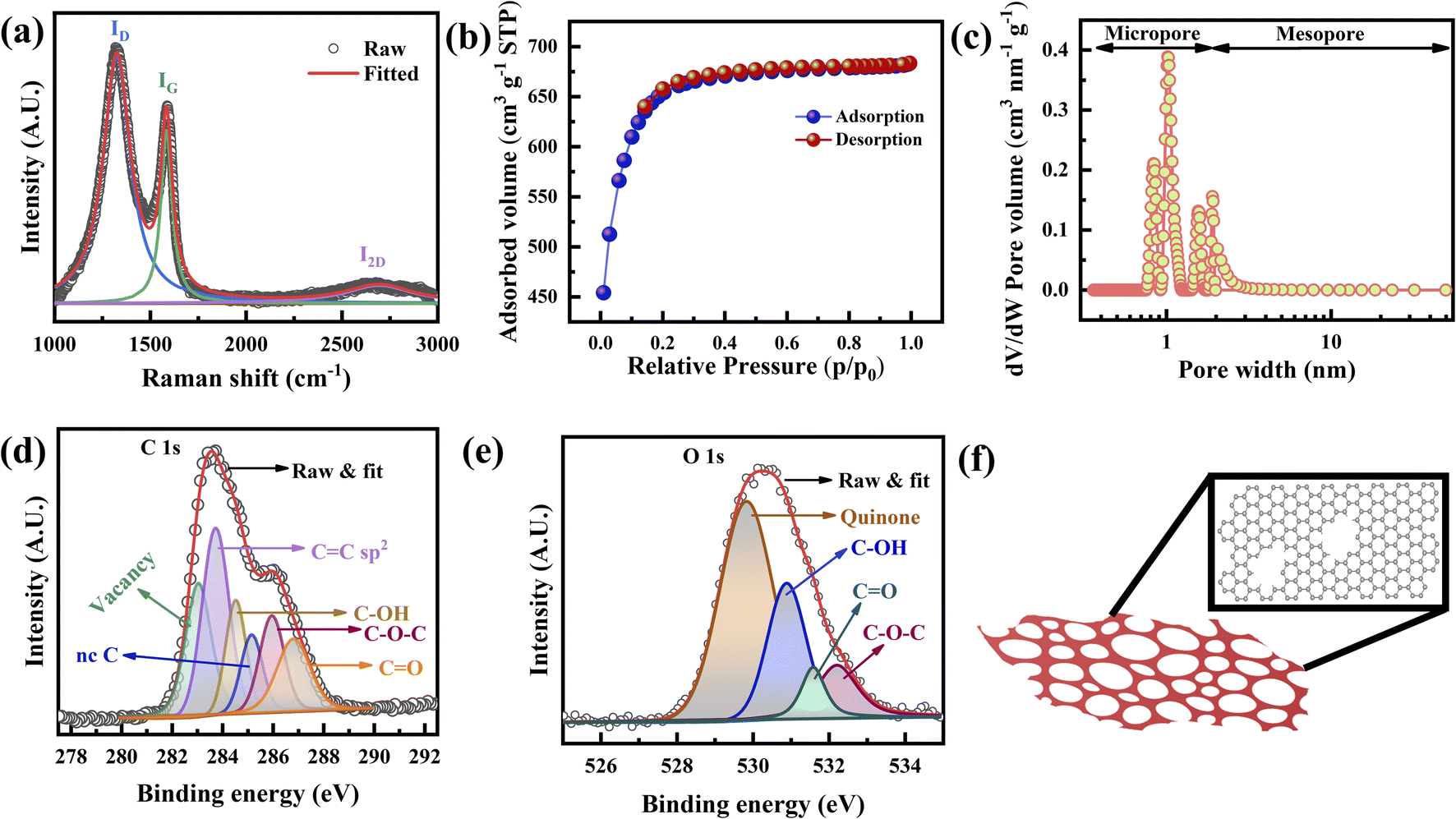Fig. 2 (a) Raman spectra of the porous graphene. (b) N₂ adsorption–desorption isotherm. (c) NLDFT pore size distribution. (d and e) C 1s and O 1s XPS spectra of the porous graphene. (f) Schematic representation of a porous graphene layer.

In other words, the 2D band can also be used to analyze the number of layers (stacking) as well as defects.^21,29–31 Four broad peaks originating from the Lorentzian fitting of the 2D band, denoted as G¹ (2533 cm⁻¹), G′ (2672 cm⁻¹), D + D′ (2839 cm⁻¹), and 2D′ (2907 cm⁻¹) as shown in Fig. S4b.†²⁵ Graphene with sufficient defects can only show the D + D′ peak, whereas the 2D′ peak appears due to momentum conservation restriction.^32,33 The full width at half maximum (FWHM) of the 2D band and the I_2D/I_G ratio clarify the stacking nature of the fabricated graphene.²¹ It is well established that the I_2D/I_G ratio is >2 for monolayer graphene, 1–2 for bilayer graphene, and <1 for FLG.^12,23 The I_2D/I_G ratio is found to be 0.10 (Fig. 2a), confirming that it is FLG.³² In addition, as the number of defects increases, the intensity of the D band increases, and that of the 2D band is suppressed.³² This will cause the I_2D/I_G ratio to decrease.

The crystallite size, L_a, defect concentration, and N_D were calculated from I_D/I_G (area ratio) to determine the charge storage ability of the graphene electrode.^25,29 The integrated intensity ratio of the D band and G band (I_D/I_G) is calculated to be 1.43, which is higher than the reported value of porous graphene foam.³⁴ The calculated L_a and N_D vary from 2.4 to 3 nm and 1.44 × 10¹² to 1.8 × 10¹² cm⁻¹, respectively, confirming the presence of highly crystallized graphene (ESI Note 1†). The intensity ratio of the D and D′ bands is found to be 3.2, revealing the presence of boundary defects.³⁵ Theoretically, the estimated carbon concentration (N_c) in graphene is 3.9 × 10¹⁵ cm⁻²; therefore, the very low carbon concentration (0.04% carbon) present in our graphene trivially affects the supercapacitor performance. Thus, XRD and Raman spectroscopy (Fig. 2a and S3, S4†) confirm that the fabricated porous graphene is mainly nanocrystalline and defective.

The specific surface area and pore size distribution of the porous graphene were analyzed using N₂ adsorption–desorption isotherms at a relative pressure (P/P₀) ranging from 0.01 to 1.0 STP (standard temperature and pressure). Fig. 2b shows the N₂ adsorption–desorption isotherm of the porous graphene, which manifests a type I isotherm with a H₄ hysteresis loop according to the IUPAC classification.^3,36,37 At P/P₀ < 0.15, the excessive inclination of the isotherm indicates the existence of a microporous structure, whereas a negligible hysteresis loop at a relative pressure P/P₀ of 0.15–0.8 STP confirms the presence of mesoporosity.^38,39 The porous graphene produced in this study achieves a total BET surface area (S_BET) of 2266 m² g⁻¹ with a total pore volume of 1.05 cm³ g⁻¹. S_BET is the combination of the micropore surface area (S_micro) and external surface area (S_ext). Therefore, the t-plot method was applied to calculate S_micro and S_ext at P/P₀ ranging from 0.1 to 0.27 STP (Fig. S5a†),^40,41 and it was found that S_micro and S_ext are 1585 and 681 m² g⁻¹, respectively. Based on the BJH model, the average mesopore width is ∼2.06 nm (Fig. S5b†).

The pore size distribution determination of the fabricated graphene was carried out using nonlocal density functional theory (NLDFT) and the result is shown in Fig. 2c, where the porous graphene shows predominantly microporous nature rather than mesoporous nature (Fig. S5c†). Based on the NLDFT calculations, the pore width of the fabricated graphene is distributed between 0.85 nm and 1.9 nm, which is compatible with the TEM observations (Fig. 1d, e and S5c†).⁴² The pore volumes based on the NLDFT calculations range from 0.21 cm³ g⁻¹ to 0.16 cm³ g⁻¹, corresponding to pore widths of 0.85 nm to 1.9 nm (Fig. S5c and Table S1†). The total micropore area of the fabricated graphene calculated from NLDFT is 1603 m² g⁻¹ (71% of the total BET surface area). It should be noted that the pore width is 1.02 nm from the NLDFT calculations and graphene possesses a large pore volume as well as a high surface area that can access a large number of electrolyte ions such as K⁺ (hydrated ion size of 0.33 nm) and OH⁻ (hydrated ion size of 0.30 nm) (Fig. S5c–e and Table S1†).^36,43

X-ray photoelectron spectroscopy (XPS) examination was carried out to investigate the presence of defects as well as the vacancies of the porous graphene. The C 1s spectra of the fabricated graphene (Fig. 2d) consist of C=C, C–OH, C–O–C, and C=O peaks at 283.73, 284.52, 285.95, and 286.81 eV, respectively. High-temperature treated graphitic structures are more prone to absorbing atmospheric moisture. The water molecules present are more reactive at the defect sites, grain boundaries and edges, resulting in the functional groups shown in the XPS spectra. It has been reported that single or multi-carbon vacancies in the hexagonal lattice and nearest neighbor plane create a chemical shift that causes peak broadening (due to the presence of defects⁴⁴) and a blue-shift of the C 1s peak.⁴⁵ Therefore, the peak at 285.15 eV is assigned to non-conjugated carbon bonding (nc–C) and/or C–H hydrogen bonding, which are known as graphite defects.^46,47 Additionally, the peak at 283.04 eV is attributed to the point defects at the pentagon and heptagon rings.⁴⁸ Excluding the peaks related to the functional groups, the total defect concentration of the fabricated graphene is ∼31%, in which nc–C and point defects related to pentagon and heptagon rings contribute 9% and 22%, respectively. Fig. 2e shows the O 1s spectra in which the peaks at 529.83, 530.89, 532.21, and 531.59 eV correspond to quinone, C–OH, C=O, and C–O–C.⁴⁹ The results of the Raman and XPS analyses (Fig. 2a, d, and e) confirm that the boundary defects are the dominant defects in the fabricated graphene.

3.3 Electrochemical examinations of the graphene electrode

The electrochemical performances of the porous graphene electrodes were studied by cyclic voltammetry (CV) and the galvanostatic charge–discharge (GCD) method using a three-electrode cell system with different concentrations of the KOH electrolyte, where the porous graphene, platinum, and Ag/AgCl were used as the working electrode, counter electrode and reference electrode, respectively. The electrode material shows nearly rectangular I–V (current–voltage) characteristics at a 1 V potential window when the electrolyte concentration varies from 0.1 M to 6.0 M, indicating capacitor-like behaviour (Fig. 3a). It is also observed that the current response increases with the KOH concentration from 0.1 to 1.0 M, leading to a more rectangular I–V curve and an increase in specific capacitance.⁵⁰ However, the reverse phenomenon is observed when the KOH concentration further increases to 6 M. This synergistic behaviour is not only controlled by the Helmholtz model but also depends on the Gouy–Chapman–Stern model and space charge (quantum capacitance) model. According to the Helmholtz model, the surface charge of the electrode is proportionate to the counter ion adsorption of the electrolyte (formation of a monolayer), whereas the Gouy–Chapman–Stern model describes the total charge balanced by the addition of a diffusion layer. Therefore, the total capacitance is the combination of the Helmholtz layer capacitance (C_H), diffuse layer capacitance (C_D), and quantum capacitance (C_Q).^16,51 It was reported that lower ionic conductivity upsets the specific capacitance for lower concentrations of the electrolyte, whereas the diffusion layer contributes predominantly at high molar concentrations.^16,52,53 The behaviour in Fig. 3a follows the previously published literature. The CV curves tend to attain an extended ellipsoid shape from a rectangular shape, as indicated in Fig. 3a and S6a–e.† In addition to electrolyte concentration, such shape changes strongly depend on the viscosity of the electrolyte and the pore sizes of the electrode. During an increase in scan rate, the current (I) increases linearly (I = Cγ, where γ is the scan rate and C is the EDL capacitance) for all KOH concentrations, resulting in almost symmetrical cathodic and anodic current responses, confirming the scan rate-independent charge storage (Fig. S6a–e†).⁵⁴ The calculated specific capacitances, C_sp, of the electrode are 60, 68, 348, 352, and 216 F g⁻¹ at the KOH concentrations of 0.1, 0.5, 1.0, 2.0, and 6.0 M at a scan rate of 5 mV s⁻¹, respectively (Fig. S6f†). This behaviour indicates that the optimum amount of charge storage requires the effective accumulation of ions on the porous graphene surfaces, which would result in specific capacitance enhancement. When the scan rate increases to 100 mV s⁻¹, the capacitance retention reduces from 52% to 34% for KOH concentrations ranging from 0.1 to 6.0 M. The capacitance retention decreases due to insufficient time to accumulate ions into the porous surface at high scan rates.

Fig. 3 (a) Cyclic voltammetry of the electrode with different electrolyte concentrations at a 10 mV s⁻¹ scan rate. (b) Capacitance vs. square root of scan rate. (c) Rate-independent specific capacitance calculated from (b). (d) Galvanostatic charge–discharge comparison with different electrolyte concentrations at a current density of 2 A g⁻¹. (e) Capacitance vs. square root of discharge time. (f) Rate-independent specific capacitance calculated from (e).

Comparative GCD studies also support the better performance of the electrode using 1.0 M KOH (Fig. 3d and S7a–e†). It exhibits a lower voltage drop and extended charge–discharge time in comparison to those with the other electrolyte concentrations. Fig. 3d shows that at all electrolyte concentrations, the GCD profiles are almost triangular due to the good coulombic efficiency. Defective microporous graphene enhances the faradaic/non-faradaic reaction sites on the surface/near-surface region, constrains the ion diffusion path, and improves the conductive pathways. The calculated specific capacitances, C_sp, from the GCD curves are shown in Fig. S7f,† where the current density varies from 2 to 30 A g⁻¹. At 2 A g⁻¹, the C_sp values are 69, 100, 540, 453 and 265 F g⁻¹ for 0.1, 0.5, 1.0, 2.0 and 6.0 M KOH, respectively (Fig. S7f†). The enhanced specific capacitance using 1.0 M KOH is due to the optimized number of the charged ions stored in the porous surface. When the electrolyte concentration increases from 0.1 to 1.0 M, ion migration within the electrode layer would be easier, leading to the feasible formation of a double-layer, resulting in an increase in C_sp. It is observed that the K⁺ ions in an aqueous solution have some interaction with water molecules as well as OH⁻ ions through the influence of van der Waals forces and Coulomb forces, respectively. This phenomenon would affect ion activity; therefore, the electrolyte ions might possess trivial charges due to their fragile interaction with water molecules. Besides the ion activity, the ion mobility depends on the ionic radii, counter ions, solvent nature, etc. in accordance with the Stokes–Einstein relation.^55,56 Consequently, by further increasing the concentration (up to 6.0 M), the ion activity may be reduced by the reduction of water hydration, leading to reduced ion mobility. As a result, K⁺ ions accumulated inside the pore decrease, causing a reduction in C_sp.⁵⁷ Therefore, an optimal electrolyte concentration (1.0 M) produces higher specific capacitance. The specific capacitances of the electrode at 10 A g⁻¹ are about 29%, 59%, 51%, 50% and 40% of the values at 2 A g⁻¹ for 0.1, 0.5, 1.0, 2.0 and 6.0 M KOH, respectively (Fig. S7f†). That is, the electrode at low current density has higher specific capacitance compared to those at higher current densities for all electrolyte concentrations. This is due to the time limitation of ion accumulation at the electrode surface.

The CV and GCD performances (Fig. 3a, d and S6, S7†) of the electrode are well in agreement with each other, although the calculated specific capacitances differ due to the different measurement techniques.⁵⁸ The total capacitances are the combination of the rate-independent (EDL) capacitance contribution, m₁, and faradaic contribution, m₂, as given by the following equation:⁸

where C represents the total capacitance in (F g⁻¹) and γ represents the scan rate (V s⁻¹).

Fig. 3b presents the variation in the specific capacitance of the electrode with the scan rate at different electrolyte concentrations. The capacitive contributions, m₁, are calculated by CV using eqn (1), when for the different concentrations of the electrolyte, as shown in Fig. 3c. It indicates that the highest capacitive contribution (130 F g⁻¹) is at 1.0 M KOH (Fig. 3c). Similarly, the capacitive contribution can also be calculated by GCD analysis. Fig. 3e indicates the variation in specific capacitance with the discharge time at different electrolyte concentrations. At γ = t^−1/2, the capacitive contribution can be calculated from eqn (1), when t^1/2 = 0. Fig. 3f presents the capacitive contribution varying with electrolyte concentration. The use of the 1 M KOH electrolyte contributes the highest capacitance (151 F g⁻¹) in comparison to the other concentrations of the electrolyte. It is indicated that the rate-independent capacitance dominates over the faradaic contributing capacitance due to the inconspicuous redox reaction (Fig. 3c and f). Therefore, from the consideration of capacitance domination, regardless of electrolyte concentration, the porous graphene electrode always shows EDLC-type behaviour.

To understand the electrolyte concentration effect on the behaviour of the porous graphene electrode, EIS measurement was carried out at a frequency range of 0.1 Hz to 0.1 MHz. Fig. 4a shows the Nyquist plot of the electrode with varying electrolyte concentration at −0.5 V. It exhibits that in all concentrations, the impedance spectra show a semicircle in the higher frequency range and inclination in the lower frequency range, revealing that the capacitance is hybrid. All the measured EIS results are fitted by an equivalent circuit, as shown in Fig. 4b, where the intercept along the Z′ axis represents the internal resistance (R_s) and the diameter of the semicircle represents the charge transfer resistance (R_ct) (CPE = constant phase element and W = Warburg element). Since R_s is independent of electrolyte concentration, R_ct can play a crucial role in the charge storage mechanism. The value of R_ct is extracted based on the equivalent circuit when the applied voltage varies from 0 to −1 V (Fig. 4b, c and S8†). It shows that R_ct varies independently of voltage. For the 0.1 M concentration, R_ct exhibits the highest value (∼15 Ω). On further increasing the concentration, the R_ct decreases to ∼10 Ω when the electrolyte concentration is 1.0 M and remains almost the same for higher concentrations (6.0 M). As shown in Fig. 4a, when the concentration increases from 0.1 to 6.0 M, the lower frequency region of the EIS curve becomes more vertical (i.e. the slope increases with increasing concentration), indicating that the EDL controls the charge storage. Fig. 4d presents the Bode plot of the electrode at −0.5 V when the electrolyte concentration varies from 0.1 to 6.0 M to visualize the characteristic frequency (knee frequency, f₀). This knee frequency is the critical frequency at a phase angle of 45° in which the capacitive and resistive behaviours become the same for energy storage devices. Therefore, the relaxation time constant τ₀ (1/2πf₀) can be calculated, which is when a supercapacitor device requires a minimum discharge time with ∼50% efficiency.⁵⁹ Fig. 4e presents the variation of the calculated relaxation time constant with potential, indicating that below 1.0 M, the tendencies of τ₀ variation become similar, whereas it becomes constant in the case of 6.0 M. In 2.0 M, above −0.4 V, τ₀ varies constantly and then starts to rise with increasing potential below −0.4 V. A similar phenomenon is observed in 1.0 M, where τ₀ varies constantly up to −0.6 V and starts rising to reach a maximum value at −1.0 V. These results confirm that the electrode at high electrolyte concentration has a good charge–discharge capability due to its higher conductivity and minimum time to discharge all energy with an efficiency higher than 50%. From the above phenomena, it is concluded that the electrodes at 1.0 M and 6.0 M KOH possess the lowest R_ct due to their higher conductivity, while that at 6.0 M KOH, there is stable τ₀ variation.

Fig. 4 (a) Electrochemical impedance spectra of the porous graphene material at a voltage of −0.5 V for varying electrolyte concentration (symbols represent the measured data and the solid line represents the fitted data based on an equivalent circuit). (b) Equivalent circuit diagram to fit the EIS spectra. (c) Variation of R_ct with potential for the different concentrations of the electrolyte. (d) Comparison of the Bode plots of the porous graphene at various concentrations of the electrolyte. (e) Variation of relaxation time with potential for the different concentrations of the electrolyte.

3.4 Charge storage mechanism of the supercapacitors

The predicted specific capacitance can be calculated based on a measured BET surface area as follows:⁶⁰where the surface area and specific capacitance are in terms of m² g⁻¹ and F g⁻¹, respectively. The electrode with the 1.0 M KOH electrolyte possesses the highest specific capacitance (540 F g⁻¹), exceeding the theoretically predicted capacitance value (474 F g⁻¹) from eqn (2), as shown in Fig. S7f.† Such a high specific capacitance may be due to the high surface area (almost equal to the theoretical surface area), optimized pore size, and defects of the fabricated graphene. A previous report indicated that the surface area-dependent specific capacitance varies linearly with pore width, and the electrode material with a pore width less than 0.7 nm contributes maximum EDL capacitance due to the non-solvated ion situated in the pore.^61,62 In this manner, by using NLDFT calculations at λ = 0, we have obtained the lowest and highest pore width of 0.85 and 1.9 nm, respectively (see ESI Note 2†). The highest micropore surface area of 765 m² g⁻¹ is obtained for the pore width of 1.02 nm at λ = 0. Therefore, the specific capacitance contribution was calculated based on the micropore surface area of the porous graphene, revealing that the electrode contributes a maximum specific capacitance of 182 F g⁻¹ at 1.0 M KOH, which reduces to 23 F g⁻¹ when the concentration reduces to 0.1 M, at a 1.02 nm pore width, due to the reduction of solvated ions (Fig. 5a). When the concentration increases 3 times (6 M), the capacitance reduces to half (89 F g⁻¹) of that at 1.0 M at 1.02 nm due to the increase in solvated ion repulsion.

Fig. 5 (a) Capacitance contribution based on the surface area associated with each pore size at a current density of 2 A g⁻¹. (b) Schematic of the hydrated K⁺ ion behaviour inside the graphene layers.

The possible reason for the decrease in d spacing due to K⁺ ions is given below. The two adjacent graphene layers can be stacked in either AA stacking or AB stacking via van der Waals interactions, with binding energies of −0.054 and 0.047 eV per atom for AA and AB, respectively.⁶³ Density functional theory (DFT) calculations indicates that the interlayer distance between adjacent layers is controlled by the hydrated K⁺ ions and aromatic ring, known as cation–π interaction.^43,64,65 The calculated hydration energy for K⁺(H₂O)₆ is −43.3 kcal mol⁻¹, whereas other hydrated cations such as Na⁺ (hydrated ion size of 0.358 nm) and Li⁺ (0.382 nm) have the hydration energies of −68.2 and −94.9 kcal mol⁻¹, respectively. The interaction energy between the graphene sheets is −39.6 kcal mol⁻¹, which is close to the hydration energy of K⁺ ions.⁴³. Consequently, K⁺ ions can easily commutate inside the graphene layers during the charge/discharge process. By contrast, the extended d spacing of graphene can accumulate a large number of hydrated K⁺ ions. Therefore, hydrated K⁺ ions intercalate into the graphene sheets and drag the two graphene layers closer to each other due to the energy difference between K⁺(H₂O)₆ and the graphene interaction energy, resulting in a slight decrease in interlayer spacing with the structural changes of K⁺(H₂O)₆.^65,66 The hydrated K⁺ ions might also enter the pore due to the cation–π interaction, although robust repulsion forces between the two hydrated cations prevent further cation insertion.^64,66 Therefore, step by step, a narrower spacing between graphene layers is filled by hydrated K⁺ ions to reach an optimum value and finally prevent pore filling.⁶⁵ These phenomena are shown in Fig. 5b. For lower concentrations, water molecules may fill the pore due to the difference between the hydration and interaction energies. Fig. 3a shows the reduced CV of 6.0 M KOH in comparison to those of 1.0 and 2.0 M KOH. This may be explained by the fact that a sufficient number of electrolyte ions are blocked from entering the graphene pore, i.e. the ion sieving effect.⁶⁷ Therefore, the specific capacitance is influenced by the suitable pore size associated with the surface area, type and concentration of electrolyte ions, and the hydration size of the ion.

To further investigate the charge storage mechanism, the electrolyte ion diffusion coefficient is studied, which is one of the parameters of the ion adsorption/desorption phenomenon. Since porous electrodes are accompanied by void space, the diffusion coefficient in the bulk electrolyte (D_bulk) is different from the in-pore diffusion coefficient of the electrolyte. Therefore, the calculated effective diffusion coefficient (D_eff) associated with each pore size is represented in Fig. 6a and S9† during the intercalation and deintercalation processes. The pores are initially filled by the electrolyte, i.e. D_bulk = D_eff (initial voltage, −1.0 V), and then D_eff reduces when the voltage changes from −1.0 to −0.9 V in all concentrations during the intercalation process (Fig. 6a), which implies the formation of a Helmholtz layer. With the voltage rising up to −0.8 V, the increase in D_eff reveals the formation of the diffusion layer, confirming that the charge storage is dominated by the diffusion of electrolyte ions. It is also shown in Fig. 6a that D_eff becomes steady at a potential of −0.7 to 0 V, confirming that the ion accumulation reaches its maximum value, attributed to the limit in the diffuse layer thickness. A similar behaviour can be seen during the deintercalation process in all electrolyte concentrations: as the Helmholtz layer formed initially, the increasing voltage from −0.3 to −1.0 V led to a steady change in D_eff with potential due to the reduction of the diffusion layer thickness, which confirms that the charges depleted in the pores (Fig. 6a and S9†). Such behaviour is observed for other pores, proving that the formation of the Helmholtz layer and diffusion layer is independent of the pore size (Fig. S9†). The overall D_eff variation decreases with increasing electrolyte concentration (1.0 to 6.0 M) due to the increase in the viscosity of the electrolyte following the Stokes–Einstein relation.

Fig. 6 (a) Effective diffusion coefficient variation with potential at varying electrolyte concentrations associated with the pore size of 1.02 nm (solid symbols represent intercalation and open symbols represent deintercalation). (b) Variation of the charge storage parameter X with potential. (c) The schematic charge storage mechanism of the porous surface.

During the charge–discharge process, electrode charges are balanced by the electrolyte ionic charges within the pores via the adsorption of counter ions, desorption of co-ions, and ion permutation.⁶⁸ Various experimental methods such as in situ NMR, eQCM, in situ XRT, in situ SAXS, and simulations can provide the possible charge storage mechanism via the change in cation and anion concentrations.^52,68–70 For higher electrolyte concentrations, porous electrodes are filled with the bulk electrolyte, whereas the electrode image forces at lower concentrations attract both cations and anions, resulting in an initial increase in the ion concentration inside the pore. As the potential increases, positive/negative ion permutation dominates for higher concentrations of the electrolyte, while co-ion desorption takes the lead for lower concentrations of the negative electrode.^52,68 To understand the charge confinement inside the pore, the parameter X can be calculated using the equation:^52,68

where D_eff(V) and D_eff(V₀) are the diffusion coefficients of the ions in the electrolyte at the potentials V and V₀, D_eff(K⁺)(V) and D_eff(OH⁻)(V) are the diffusion coefficients of the cation, K⁺, and anion, OH⁻, at potential V, and D_eff(K⁺)(V₀) and D_eff(OH⁻)(V₀) are the diffusion coefficients of the cation and anion at potential V₀, respectively. Ideally, a positive value of X represents counter ion adsorption, while a negative value indicates co-ion desorption, and zero indicates the ion permutation mechanism. Fig. 6b presents the calculated X of the porous graphene at a pore size of 1.02 nm in all electrolyte concentrations during the charging process. Initially, at a potential of −1.0 V, equal amounts of K⁺ and OH⁻ are filled inside the pore. At a −0.9 V potential, in all concentrations, the calculated X reaches a positive value, which implies K⁺ ion adsorption inside the pore. With further increase in potential (−0.8 V), X becomes negative in all concentrations except 1.0 and 2.0 M, implying that OH⁻ ions move outside the pore. The more positive response of X at 1.0 and 2.0 M with −0.8 V is responsible for more K⁺ ion accumulation inside the 1.02 nm pore. When the potential reaches −0.7 V, the positive X for the concentrations of 0.1, 0.5, and 6.0 M corresponds to K⁺ ion adsorption, whereas the negative X for the concentrations of 1.0 and 2.0 M is responsible for OH⁻ ion desorption. With an increase in potential from −0.6 to 0 V, X varies near the zero region, revealing that K⁺ and OH⁻ ion permutation takes place. It should be noted that the ion adsorption and desorption mechanisms occur for the potential range between −1.0 and −0.6 V, whereas the ion permutation mechanism is seen in the potential range between −0.6 and 0 V due to the non-equilibrium state of the K⁺ and OH⁻ ion concentrations inside the pores, although the overall charge balance is present for different pores (Fig. S10†). OH⁻ ion desorption happens at the pore sizes of 0.85 and 1.02 nm, whereas K⁺ ion adsorption takes place in 1.9 nm pores to achieve overall charge balance, and ion permutation occurs in 1.6 nm pores in the 0.1 M KOH concentration (Fig. S10a†) with a potential increase from −0.9 V to −0.8 V; thereafter, ion permutation takes place up to 0 V. In the case of the 0.5 M concentration, the total charge balance occurs via K⁺ ion adsorption in 0.85 nm pores and OH⁻ desorption in 1.02, 1.6, and 1.9 nm pores in the potential range of −0.9 V to −0.7 V (Fig. S10b†). A different charge storage phenomenon is observed in the 1 M electrolyte concentration. At this concentration, initially, K⁺ ions adsorb in the pore sizes of 0.85 and 1.02 nm, and subsequently, OH⁻ desorption takes place in the pore sizes of 1.6 and 1.9 nm when the potential varies from −0.9 V to −0.8 V, as shown in Fig. S10c.† By further increasing the potential to −0.4 V in 1.0 M KOH, alternative desorption of OH⁻ and adsorption of K⁺ take place together in the pore sizes of 0.85 nm and 1.02 nm; meanwhile, the reverse phenomena occur in the pore sizes of 1.6 nm and 1.9 nm, respectively, for the sake of total charge balance (Fig. S10c†), while adsorption phenomena are shown in the pore sizes of 0.85, 1.02 and 1.9 nm and equivalent desorption is observed in the 1.6 nm pores for 2.0 M KOH, as shown in Fig. S10d.† Similarly, for 6.0 M KOH, adsorption is seen in the 0.85 and 1.6 nm pores, and equivalent desorption is revealed in 1.02 and 1.9 nm pores (Fig. S10e†). Based on the above discussion, the schematic charge storage mechanisms for the adsorption of counter ions, desorption of co-ions, and ion permutation are presented in Fig. 6c. Therefore, it can be concluded that the alternate adsorption–desorption of K⁺ and OH⁻ ions for the 1 M concentration provides higher specific capacitance.

For energy storage applications, a symmetrical solid-state supercapacitor has been fabricated, where two identical porous graphene electrodes made in this study are used as the cathode and anode and a PVA–KOH-based polymer gel is used as the electrolyte. Fig. 7a presents the CV curves at various scan rates from 5 to 200 mV s⁻¹ with a potential window of 1.5 V. It is indicated that all the CV curves show a nearly rectangular shape, confirming that the device exhibits an EDLC nature. A similar behaviour is found for the GCD characteristics, where all the GCD curves display a linear voltage response at various current densities from 0.1 to 3 A g⁻¹ (Fig. 7b). According to the calculation of the GCD profile, the supercapacitor shows a specific capacitance of 58 F g⁻¹ at 0.1 A g⁻¹. When the current density increases to 3 A g⁻¹, the device exhibits a specific capacitance of 31 F g⁻¹ with a retention of up to 53% (Fig. 7c). For lower current densities, ion movement is slower during charging, resulting in a large amount of charges accumulating on the porous surface. When the current density becomes high, ions move faster, leading to a short time for charge accumulation on the porous surface, resulting in lower specific capacitance. Fig. 7d presents the Ragone plot of the supercapacitor, indicating linear variation. It delivers an energy density of 18 W h kg⁻¹ at a 300 W kg⁻¹ power density, and a maximum power density of 10.2 kW kg⁻¹ at a 7 W h kg⁻¹ energy density. The Nyquist plot confirms the internal and charge transfer resistances of the device (Fig. 7e). It shows an internal resistance of ∼2.73 Ω and a charge transfer resistance of ∼16.6 Ω. The resistance values of this gel electrolyte supercapacitor are higher than those of the ones with liquid electrolytes. Fig. 7f presents the cycling stability and coulombic efficiency of the supercapacitor. It delivers almost 100% capacitance retention and coulombic efficiency after 6000 cycles. The electrodes of the supercapacitor with a porous structure and defects provide additional active sites for electrolyte ions, leading to improved charge storage. Such stable performance may be caused by stable ionic charge movement and accumulation in the pores.

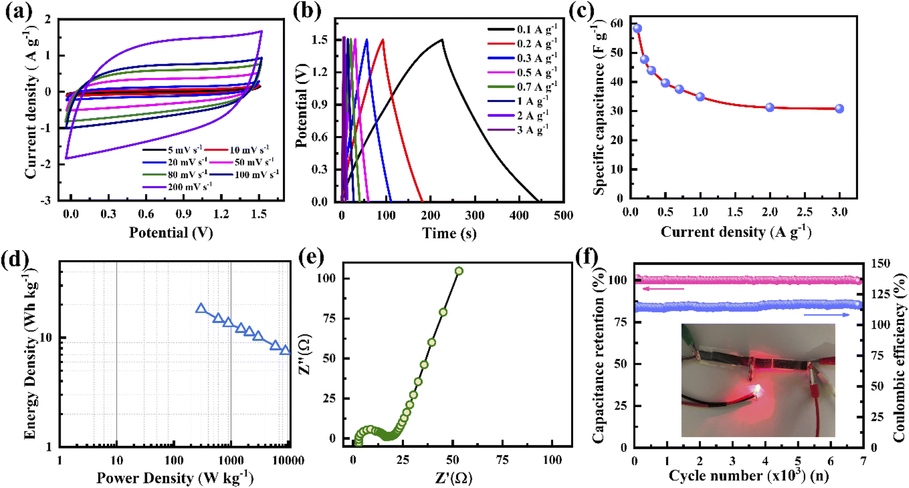Fig. 7 (a) Cyclic voltammetry of the symmetrical supercapacitor with porous graphene electrodes and PVA–KOH-based electrolyte at various scan rates. (b) Galvanostatic charge–discharge of the supercapacitor at various current densities. (c) The specific capacitance of the supercapacitor. (d) Ragone plots of the supercapacitor. (e) Nyquist plots of the supercapacitor. (f) Long cycling performance of the supercapacitor. A light-up LED using the supercapacitor (inset).

4. Conclusions

Microporous graphene was successfully synthesized at 950 °C via the pyrolysis method. BET surface area and NLDFT calculations confirmed that the fabricated graphene possesses a high surface area of 2266 m² g⁻¹ with pore sizes in the range of 0.85 to 1.9 nm. The electrode made using this porous graphene exhibited a maximum specific capacitance value of 540 F g⁻¹ at 2 A g⁻¹ using a 1.0 M KOH electrolyte. By varying the KOH electrolyte concentration, the specific capacitance of the electrode was also changed. The effective diffusion coefficients of the electrolyte ions were used to confirm the charge storage mechanism, which was the adsorption, desorption, and permutation of electrolyte ions. A symmetrical solid-state supercapacitor device fabricated with the above-mentioned electrodes and PVA–KOH-based electrolyte exhibited the energy and power densities of 18 W h kg⁻¹ and 10.2 kW kg⁻¹, respectively, with a capacitance retention and coulombic efficiency of 100% after 6000 cycles. This study not only presents a high-performing supercapacitor but also provides its charge storage mechanism. This can establish the direction of fabricating new electrode materials with optimized pores and suitable electrolytes to produce high-performance supercapacitors.

Author contributions

T. Y. T., K. H. W., and T. W. raised the idea and directed the study. B. P. carried out all the experimental work and analyzed the data with the help of D. P. and F. M. S. P. A. L. assisted with the collection of some experimental data. B. P. wrote the manuscript and T. Y. T. corrected and finalized the manuscript. All the authors reviewed the final manuscript.

Conflicts of interest

There are no conflicts to declare.

Acknowledgements

This study was partially supported by the Ministry of Science and Technology, Taiwan, under project number 109-2221-E009-034-MY3. This work was also supported by the Higher Education Sprout Project of the National Yang Ming Chiao Tung University and Ministry of Education (MOE), Taiwan.

References

1. Z. Yu, Y. Feng, D. Feng and X. Zhang, Microporous Mesoporous Mater., 2021, 312, 110781.
2. M. L. Divya, Y.-S. Lee and V. Aravindan, ACS Energy Lett., 2021, 6, 4228–4244.
3. X. Lei, M. Wang, Y. Lai, L. Hu, H. Wang, Z. Fang, J. Li and J. Fang, J. Power Sources, 2017, 365, 76–82.
4. V. Skrypnychuk, N. Boulanger, A. Nordenström and A. Talyzin, J. Phys. Chem. Lett., 2020, 11, 3032–3038.
5. M. Salanne, B. Rotenberg, K. Naoi, K. Kaneko, P.-L. Taberna, C. P. Grey, B. Dunn and P. Simon, Nat. Energy, 2016, 1, 16070.
6. K. Breitsprecher, M. Janssen, P. Srimuk, B. L. Mehdi, V. Presser, C. Holm and S. Kondrat, Nat. Commun., 2020, 11, 6085.
7. D. Sarkar, D. Das, S. Das, A. Kumar, S. Patil, K. K. Nanda, D. D. Sarma and A. Shukla, ACS Energy Lett., 2019, 4, 1602–1609.
8. T. Lin, I.-W. Chen, F. Liu, C. Yang, H. Bi, F. Xu and F. Huang, Science, 2015, 350, 1508–1513.
9. D. W. Kim, J. Choi, D. Kim and H.-T. Jung, J. Mater. Chem. A, 2016, 4, 17773–17781.
10. H. Chang, J. Kang, L. Chen, J. Wang, K. Ohmura, N. Chen, T. Fujita, H. Wu and M. Chen, Nanoscale, 2014, 6, 5960–5966.
11. A. Idowu, B. Boesl and A. Agarwal, Carbon, 2018, 135, 52–71.
12. H. Kashani, Y. Ito, J. Han, P. Liu and M. Chen, Sci. Adv., 2019, 5, eaat6951.
13. H. Bi, Z. Liu, F. Xu, Y. Tang, T. Lin and F. Huang, J. Mater. Chem. A, 2016, 4, 11762–11767.
14. N. F. Sylla, N. M. Ndiaye, B. D. Ngom, D. Momodu, M. J. Madito, B. K. Mutuma and N. Manyala, Sci. Rep., 2019, 9, 13673.
15. J. Chmiola, G. Yushin, Y. Gogotsi, C. Portet, P. Simon and P. L. Taberna, Science, 2006, 313, 1760–1763.
16. H. Shao, Y.-C. Wu, Z. Lin, P.-L. Taberna and P. Simon, Chem. Soc. Rev., 2020, 49, 3005–3039.
17. X.-F. Jiang, X.-B. Wang, P. Dai, X. Li, Q. Weng, X. Wang, D.-M. Tang, J. Tang, Y. Bando and D. Golberg, Nano Energy, 2015, 16, 81–90.
18. S. N. Chiu, Mater. Charact., 1995, 34, 149–165.
19. M. A. Worsley, T. T. Pham, A. Yan, S. J. Shin, J. R. I. Lee, M. Bagge-Hansen, W. Mickelson and A. Zettl, ACS Nano, 2014, 8, 11013–11022.
20. Z. Q. Li, C. J. Lu, Z. P. Xia, Y. Zhou and Z. Luo, Carbon, 2007, 45, 1686–1695.
21. T. M. Paronyan, A. K. Thapa, A. Sherehiy, J. B. Jasinski and J. S. D. Jangam, Sci. Rep., 2017, 7, 39944.
22. C. N. R. Rao, K. Biswas, K. S. Subrahmanyam and A. Govindaraj, J. Mater. Chem., 2009, 19, 2457.
23. L. L. Zhang, X. Zhao, H. Ji, M. D. Stoller, L. Lai, S. Murali, S. Mcdonnell, B. Cleveger, R. M. Wallace and R. S. Ruoff, Energy Environ. Sci., 2012, 5, 9618.
24. A. W. Robertson and J. H. Warner, Nano Lett., 2011, 11, 1182–1189.
25. A. C. Ferrari, Solid State Commun., 2007, 143, 47–57.
26. P. Xu, Q. Gao, L. Ma, Z. Li, H. Zhang, H. Xiao, X. Liang, T. Zhang, X. Tian and C. Liu, Carbon, 2019, 149, 452–461.
27. M. J. Matthews, M. A. Pimenta, G. Dresselhaus, M. S. Dresselhaus and M. Endo, Phys. Rev. B: Condens. Matter Mater. Phys., 1999, 59, R6585–R6588.
28. A. C. Ferrari and J. Robertson, Phys. Rev. B: Condens. Matter Mater. Phys., 2001, 63, 121405.
29. A. C. Ferrari and D. M. Basko, Nat. Nanotechnol., 2013, 8, 235–246.
30. L. M. Malard, M. A. Pimenta, G. Dresselhaus and M. S. Dresselhaus, Phys. Rep., 2009, 473, 51–87.
31. C. H. Lui, Z. Li, Z. Chen, P. V. Klimov, L. E. Brus and T. F. Heinz, Nano Lett., 2011, 11, 164–169.
32. A. Kaniyoor and S. Ramaprabhu, AIP Adv., 2012, 2, 032183.
33. L. G. Cançado, A. Jorio, E. H. M. Ferreira, F. Stavale, C. A. Achete, R. B. Capaz, M. V. O. Moutinho, A. Lombardo, T. S. Kulmala and A. C. Ferrari, Nano Lett., 2011, 11, 3190–3196.
34. L. Lu, F. Pei, T. Abeln and Y. Pei, Carbon, 2020, 157, 437–447.
35. A. Eckmann, A. Felten, A. Mishchenko, L. Britnell, R. Krupke, K. S. Novoselov and C. Casiraghi, Nano Lett., 2012, 12, 3925–3930.
36. H. Liu, Y. Zhang, Q. Ke, K. H. Ho, Y. Hu and J. Wang, J. Mater. Chem. A, 2013, 1, 12962.
37. D. Zhang, M. Han, B. Wang, Y. Li, L. Lei, K. Wang, Y. Wang, L. Zhang and H. Feng, J. Power Sources, 2017, 358, 112–120.
38. Z. Li, S. Gadipelli, H. Li, C. A. Howard, D. J. L. Brett, P. R. Shearing, Z. Guo, I. P. Parkin and F. Li, Nat. Energy, 2020, 5, 160–168.
39. M. Mirzaeian, Q. Abbas, D. Gibson and M. Mazur, Energy, 2019, 173, 809–819.
40. A. J. Lecloux, R. Atluri, Y. V. Kolen’ko and F. L. Deepak, Nanoscale, 2017, 9, 14952–14966.
41. A. Galarneau, F. Villemot, J. Rodriguez, F. Fajula and B. Coasne, Langmuir, 2014, 30, 13266–13274.
42. G. Kupgan, T. P. Liyana-Arachchi and C. M. Colina, Langmuir, 2017, 33, 11138–11145.
43. Y. Yang, L. Mu, L. Chen, G. Shi and H. Fang, Phys. Chem. Chem. Phys., 2019, 21, 7623–7629.
44. H. Estrade-Szwarckopf, Carbon, 2004, 42, 1713–1721.
45. A. Barinov, O. B. Malcioǧlu, S. Fabris, T. Sun, L. Gregoratti, M. Dalmiglio and M. Kiskinova, J. Phys. Chem. C, 2009, 113, 9009–9013.
46. N. Lachman, X. Sui, T. Bendikov, H. Cohen and H. D. Wagner, Carbon, 2012, 50, 1734–1739.
47. K. Ganesan, S. Ghosh, N. Gopala Krishna, S. Ilango, M. Kamruddin and A. K. Tyagi, Phys. Chem. Chem. Phys., 2016, 18, 22160–22167.
48. A. Fujimoto, Y. Yamada, M. Koinuma and S. Sato, Anal. Chem., 2016, 88, 6110–6114.
49. M. Mohandoss, S. Sen Gupta, A. Nelleri, T. Pradeep and S. M. Maliyekkal, RSC Adv., 2017, 7, 957–963.
50. J. Chmiola, G. Yushin, R. Dash and Y. Gogotsi, J. Power Sources, 2006, 158, 765–772.
51. J. Xia, F. Chen, J. Li and N. Tao, Nat. Nanotechnol., 2009, 4, 505–509.
52. C. Prehal, C. Koczwara, H. Amenitsch, V. Presser and O. Paris, Nat. Commun., 2018, 9, 4145.
53. D. Weingarth, M. Zeiger, N. Jäckel, M. Aslan, G. Feng and V. Presser, Adv. Energy Mater., 2014, 4, 1400316.
54. J. Liu, J. Wang, C. Xu, H. Jiang, C. Li, L. Zhang, J. Lin and Z. X. Shen, Adv. Sci., 2018, 5, 1700322.
55. B. Pal, S. Yang, S. Ramesh, V. Thangadurai and R. Jose, Nanoscale Adv., 2019, 1, 3807–3835.
56. Y. Saito, W. Morimura, R. Kuratani and S. Nishikawa, J. Phys. Chem. C, 2016, 120, 3619–3624.
57. K.-C. Tsay, L. Zhang and J. Zhang, Electrochim. Acta, 2012, 60, 428–436.
58. B. Pattanayak, F. M. Simanjuntak, D. Panda, C.-C. Yang, A. Kumar, P.-A. Le, K.-H. Wei and T. Y. Tseng, Sci. Rep., 2019, 9, 16852.
59. K. Jiang, I. A. Baburin, P. Han, C. Yang, X. Fu, Y. Yao, J. Li, E. Cánovas, G. Seifert, J. Chen, M. Bonn, X. Feng and X. Zhuang, Adv. Funct. Mater., 2020, 30, 1908243.
60. L. Chang, W. Wei, K. Sun and Y. H. Hu, J. Mater. Chem. A, 2015, 3, 10183–10187.
61. F. Beck, M. Dolata, E. Grivei and N. Probst, J. Appl. Electrochem., 2001, 31, 845–853.
62. C. Vix-Guterl, E. Frackowiak, K. Jurewicz, M. Friebe, J. Parmentier and F. Béguin, Carbon, 2005, 43, 1293–1302.
63. M. Birowska, K. Milowska and J. A. Majewski, Acta Phys. Pol., A, 2011, 120, 845–848.
64. A. S. Mahadevi and G. N. Sastry, Chem. Rev., 2013, 113, 2100–2138.
65. L. Chen, G. Shi, J. Shen, B. Peng, B. Zhang, Y. Wang, F. Bian, J. Wang, D. Li, Z. Qian, G. Xu, G. Liu, J. Zeng, L. Zhang, Y. Yang, G. Zhou, M. Wu, W. Jin, J. Li and H. Fang, Nature, 2017, 550, 380–383.
66. X. Liu, C.-Z. Wang, H.-Q. Lin, K. Chang, J. Chen and K.-M. Ho, Phys. Rev. B: Condens. Matter Mater. Phys., 2015, 91, 035415.
67. Y. Zhang, J. Peng, G. Feng and V. Presser, Chem. Eng. J., 2021, 419, 129438.
68. A. C. Forse, C. Merlet, J. M. Griffin and C. P. Grey, J. Am. Chem. Soc., 2016, 138, 5731–5744.
69. C. Merlet, C. Péan, B. Rotenberg, P. A. Madden, B. Daffos, P. L. Taberna, P. Simon and M. Salanne, Nat. Commun., 2013, 4, 2701.
70. C. Prehal, C. Koczwara, N. Jäckel, A. Schreiber, M. Burian, H. Amenitsch, M. A. Hartmann, V. Presser and O. Paris, Nat. Energy, 2017, 2, 16215.

---

Footnote

† Electronic supplementary information (ESI) available. See https://doi.org/10.1039/d2ra04194d

---