
 Open Access Article
 This Open Access Article is licensed under a
 Creative Commons Attribution 3.0 Unported Licence
A first principles examination of phosphorescence
Anjay Manian *a,
Igor Lyskova,
Robert A. Shawb and
Salvy P. Russoa
*a,
Igor Lyskova,
Robert A. Shawb and
Salvy P. Russoa
aARC Centre of Excellence in Exciton Science, School of Science, RMIT University, Melbourne, 3000, Australia. E-mail: anjay.manian3@rmit.edu.au; salvy.russo@rmit.edu.au
bDepartment of Chemistry, University of Sheffield, Sheffield S3 7HF, UK
First published on 7th September 2022
Abstract
This paper explores phosphorescence from a first principles standpoint, and examines the intricacies involved in calculating the spin-forbidden T1 → S0 transition dipole moment, to highlight that the mechanism is not as complicated to compute as it seems. Using gas phase acridine as a case study, we break down the formalism required to compute the phosphorescent spectra within both the Franck–Condon and Herzberg–Teller regimes by coupling the first triplet excited state up to the S4 and T4 states. Despite the first singlet excited state appearing as an Lb state and not of nπ* character, the second order corrected rate constant was found to be 0.402 s−1, comparing well with experimental phosphorescent lifetimes of acridine derivatives. In showing only certain states are required to accurately describe the matrix elements as well as how to find these states, our calculations suggest that the nπ* state only weakly couples to the T1 state. This suggest its importance hinges on its ability to quench fluorescence and exalt non-radiative mechanisms rather than its contribution to the transition dipole moment. A followup investigation into the T1 → S0 transition dipole moment's growth as a function of its coupling to other electronic states highlights that terms dominating the matrix element arise entirely from the inclusion of states with strong spin–orbit coupling terms. This means that while the expansion of the transition dipole moment can extend to include an infinite number of electronic states, only certain states need to be included.
1 Introduction
Phosphorescence has the official definition of a radiative transition between states of different electronic spin multiplicities,1–6 but is more commonly understood as emission from first triplet excited state to the electronic ground state. While well known that photophysical properties of all compounds change with respect to temperature, systems prone to phosphorescence behave very differently.3,4,7–11 Interest in the photon harvesting applications of phosphorescent molecules has increased in the last few decades12–21 due to their recycling, or harvesting, of triplet excitons.In addition to temperature, the phosphorescent phenomenon displays a sensitivity to molecular aggregation effects and the access of oxygen.3–5,22–24 Consequentially, most experimental studies are conducted under cryogenic and/or air-proof conditions, which seriously limits research into new more efficient molecular species. The reach of these results affects applications in many fields including but not limited to medical, photobiological, or optoelectronic fields. The most well known and efficient phosphorescent compounds are in the organometallic family of chromophores, such as metal sulfides or metal-cored porphyrins.15,20,25–30 However, fabrication of these kinds of molecules is neither cheap nor environmentally sound. The design of bio-friendly organic compounds for phosphorescent applications which are not limited by temperature or open-air is extremely difficult as the coupling between singlet and triplet excited states is typically quite weak. The mechanism therefore cannot compete with non-radiative processes such as internal conversion (spin is conserved) or inter-system crossing (spin is not conserved).31,32 While a myriad of well known biological compounds have been reported to phosphoresce,33 the rates are very slow. Consequentially, a method which could help predict the phosphorescence related properties of a candidate chromophore would facilitate those working to fabricate a more efficient species.
The photophysics of many heterocyclic and aromatic chromophores are defined by the spacing of two similarly characterised states, denoted as La and Lb states as per Platt's notation.34 The energetic ordering or spacing of these often degenerate states can change with respect to the medium, altering fluorescence and non-radiative decay pathways, a phenomenon known as solvatochromativity.35,36 Good examples for this include diketo-pyrrolopyrrole,31,37,38 indole,39–41 and acridine,11,42 with all three displaying drastically different photophysics depending on the polarity of the solvent it is measured in. Acridine in particular is interesting as in addition to the low lying La and Lb states, there is also a low lying nπ* state. In fact, this non-bonding state has been reported to appear as the emitting state in non-polar solvents and the gas phase.11,42,43
Phosphorescence is a rare mechanism not only due to its impeding activation like temperature dependence and air-induced quenching due to oxygen contamination, but also because an exciton residing on a given excited state has to relax down to the first triplet excited state. In principle, it occurs for all compounds, but is literally outshined by fluorescence. However, if one considers the case where the fluorescing state is of nπ* character instead of ππ* character, fluorescence may be orders of magnitude smaller than the required inter-system crossing rate constant, allowing phosphorescence to compete. Further, acridine and it's derivatives has been reported to phosphoresce.11,42–48 For these reasons, we have chosen gas phase acridine, shown in Fig. 1, as a case study molecular system and will compute it's phosphorescence spectra and corresponding rate constant from first principles.
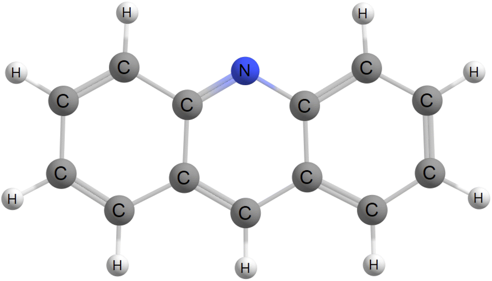 | ||
| Fig. 1 Schematic representation of the acridine chromophore. | ||
2 Theory
The rate of phosphorescence kp can be calculated using Einstein's spontaneous emission function:3,4,25,31,49,50
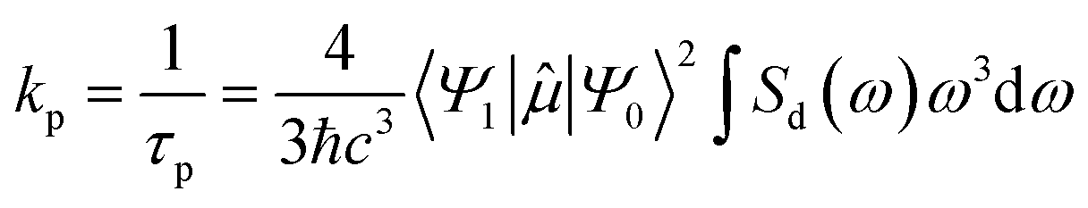 | (1) |
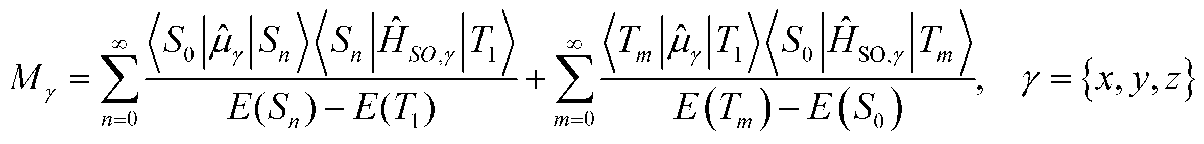
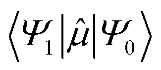 is the transition dipole moment between the initial and final states of the transition, in this case describing the T1 → S0 transition, Sd is the normalised phosphorescence emission spectra, and ω is the energy. While computation of the transition dipole moment for same spin transitions is a standard option for most quantum chemical packages, the same cannot be said concerning
 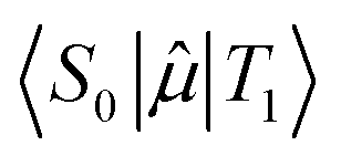 , which we will denote as M from this point onward for convenience. In order to bypass the forbidden nature of such a transition, we need to mix singlet and triplet state wavefunctions.3,4,26,29,51,52 Altering of electron spin is the result of strong spin–orbit coupling between states of different spin, so our transition dipole moment matrix elements have to be mixed with spin–orbit coupling matrix elements. If we choose to ignore vibronic effects and stay within the Franck–Condon (FC) regime,53–55 we can represent M as:
 | (2) |
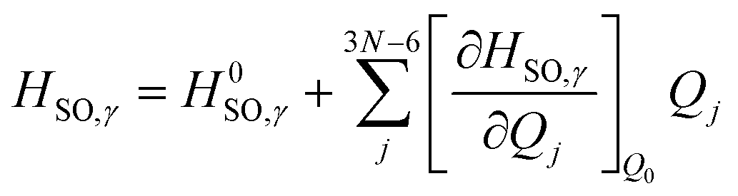
We can then begin to consider the effects that each respective vibrational normal mode has to the rate constant, within the Herzberg–Teller (HT) regime.56 As explained by Lower & El-Sayed,57 singlet states of polyatomic molecules have some degree of triplet character, while triplet states have some degree of singlet character. Because this mixing is spin forbidden, our second order correction examines the derivatives with respect to the change in the spin–orbit coupling between states. To do this, we can expand the spin–orbit coupling operator at the Franck–Condon point HSO with respect to the vibrational coordinates Qj at the equilibrium geometry Q0 using a Taylor series, truncated at the first derivative term.3,50 This gives us:
 | (3) |
Here, the first term on the righthand side mediates the FC contribution while the second term mediates the HT contribution.
3 Computational details
Optimised† geometries were computed using a Complete Active Space Self Consistent Field (CASSCF) model with 6 electrons and 6 active orbitals, averaging across 5 roots using the Karlsruhe variant of the split valence with polarisation functions on non-hydrogen atoms def2-SV(P) basis set,58,59 as implemented in the MOLPRO software package.60 MOLPRO currently does not allow for solvent models with CASSCF calculations; as such we will calculate the properties of acridine in the gas phase. The electronic Hessian was then computed by finite differences using analytical energy gradients using the same CAS window and basis set. Corrections to the singlet point energies were then obtained by using the n-electron valence perturbation theory to the second order (NEVPT2) formalism61–64 as implemented in the ORCA software package,65 with the larger Karlsruhe triple zeta valence polarised def2-TZVP basis set.66The singlet–singlet and triplet–triplet transition dipole moments were computed using the DFT based multireference configuration interaction DFT/MRCI method,67,68 using the def-SV(P) basis set. The one-particle basis was built using the Becke half-and-half Yang–Lee–Parr BHLYP exchange-correlation functional69 as implemented in the TURBOMOLE software package.70 The DFT/MRCI reference space was generated iteratively by including all electron configurations with expansion coefficients greater than 10−3 using 10 electrons across 10 orbitals for a maximum of two-electron excitations. Probe runs were calculated by discarding configurations with energy less than the highest reference energy; starting with a threshold of 0.6 Eh, then 0.8, both within a paradigm of tight parameters,68 then using a threshold of 1.0 Eh using standard parameters. Spin–orbit matrix elements were computed using the SPOCK.CI module71–73 of the DFT/MRCI platform, within a quasi-degenerate perturbation theory framework. The spin–orbit coupling terms are computed using Breit-Pauli Hamiltonians,73 further simplified using a spin–orbit mean field approximation.71 Energies and coupling terms were calculated at the Franck–Condon point with respect to the initial state i.e. the 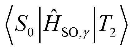 spin–orbit matrix elements were computed at the T2 optimised geometry.
It should be noted that the triplet sublevels here are assumed to be degenerate as DFT/MRCI calculations are non-relativistic. As such, no zero-field splitting effects are included in this work.
The VIBES software package74 was used to compute the phosphorescence emission spectra, using 216 integration points with a 300 fs time integral for integration, and a 100 cm−1 width for the Gaussian damping of the correlation function, all at a temperature of 300 K. For the calculation of derivative terms, numerical derivatives are calculated using a finite central difference method with a step size of h = 0.05 with respect to the mass-weighted normal coordinates. In order to account for the shifting of molecular orbital (MO) phase for each numerical derivative, a fictitious dot product was constructed using the configuration amplitudes of the leading configurations of the coupled states, and the largest MO coefficient of the underlying orbitals. Comparing these resulting products to the FC product clearly highlights when the phase has been reversed. For more details, see ref. 31 and 75.
4 Results & discussion
Upon analysis of the low lying excited states, which is summarised in Table 1, we note that none of our states are classified as an nπ* state. As shown in Fig. 2, the 6 orbitals included in the CAS window are all π type orbitals, and clearly does not include the non-bonding type highest occupied molecular orbital (HOMO). No missing orbitals were noticed within the lowest unoccupied molecular orbitals (LUMOs). Our results show that the first singlet excited state with an adiabatic energy of 3.19 eV is the Lb state as per Platt's notation, with mixed character of HOMO−1 → LUMO and HOMO → LUMO+1, while the second singlet excited state with an adiabatic energy of 3.92 eV is the La state, with a clear HOMO → LUMO character. Interestingly, the third singlet excited state with an adiabatic energy of 4.64 eV was found to be of double excitation quality as HOMO2 → LUMO2,‡ while the fourth singlet excited state with an adiabatic energy of 4.84 eV was found to be mixed between HOMO2 → LUMO2 and HOMO → LUMO character. On the triplet manifold, the T1 state with an adiabatic energy of 1.59 eV was of La character, while the second excited state with an adiabatic energy of 3.59 eV was of Lb character. The third and fourth triplet excited states, with adiabatic energies of 4.41 eV and 4.67 eV respectively, were observed as mixed with HOMO−2 → LUMO and HOMO → LUMO+2 characteristics and of HOMO−1, HOMO → LUMO2 character respectively.| State | Energy | Orbital configuration | Contribution |
|---|---|---|---|
| 1a1 | — | GS | 0.97 |
| 2a1 | 3.19 | HOMO−1 → LUMO | 0.32 |
| HOMO → LUMO+1 | 0.28 | ||
| 3a1 | 3.92 | HOMO → LUMO | 0.88 |
| 4a1 | 4.64 | HOMO2 → LUMO2 | 0.65 |
| 5a1 | 4.84 | HOMO2 → LUMO2 | 0.45 |
| HOMO → LUMO | 0.17 | ||
| 1a3 | 1.59 | HOMO → LUMO | 0.88 |
| 2a3 | 3.59 | HOMO−1 → LUMO | 0.76 |
| 3a3 | 4.41 | HOMO−2 → LUMO | 0.39 |
| HOMO → LUMO+2 | 0.15 | ||
| 4a3 | 4.67 | HOMO2 → LUMO2 | 0.51 |
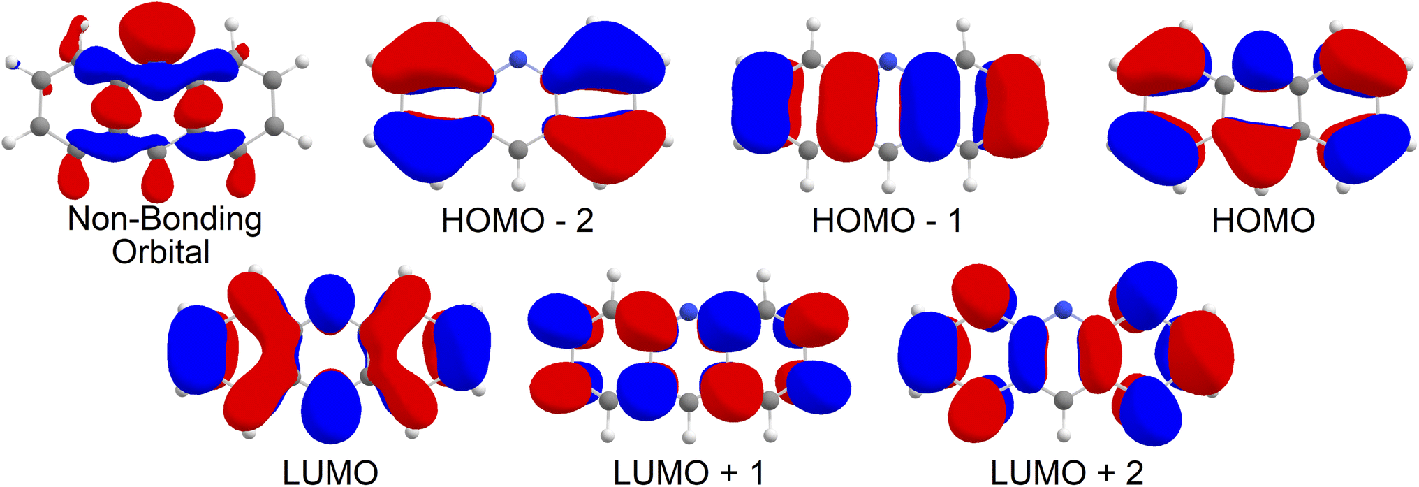 | ||
| Fig. 2 Molecular orbitals for acridine in the gas phase. | ||
Comparison of these results to work by Rubio-Pons and coworkers43 reports Lb and La singlet state energies of 3.28 eV and 3.34 eV respectively, both above an nπ* state with an energy of 3.18 eV. While initially this appears to be a cause for concern, closer observation shows the nπ* state to have a very small oscillator strength of 0.003, suggesting that the importance of this state is not in it's contribution to the strength of the T1 → S0 transition dipole moment, but rather in the quenching of fluorescence as to allow for non-radiative decay, evidence for which can be found in some spiro-compounds.76 Comparing our computed singlet energies to experimental work by Narva & McClure77 shows that while the energy of our Lb state may be reasonable, the La state is greatly overestimated. This is similarly seen for the triplet manifold as computed by Rubio-Pons and coworkers. While energies for the La triplet state published by Rubio-Pons and coworkers is within 0.2 eV of our calculated value, it is smaller by 0.4 eV as reported experimentally by Prochorow and coworkers.44 Conversely, the Lb triplet state is overestimated by 0.3 eV as reported experimentally by Kikuchi and coworkers.45 Further, it seems Rubio-Pons and coworkers also found an nπ* on the triplet manifold, appearing as the T2 state with an energy of 2.9 eV.
Investigation into why our results did not match with those reported by Rubio-Pons and coworkers shows that their calculation used a CAS window double the size of that used in this work (12,12), which is likely why the non-bonding orbital was not found within the low lying states. However, probe calculations run using the same window did not yield the expected non-bonding state either. There could be a number of reasons for this occurring, however this is currently outside the current scope of this work and will need to be reexamined in the future. Conversely for the experimental results, most phosphorescence measured for acridine is within crystalline matrices, which can be expected to have a strong effect on the photophysical properties of the compound. Juxtaposition of all these results shows a high degree of variability between data sets, and highlights the sensitivity of acridine and how strongly it can couple to its medium. Assuming the dielectric constant of 2,3-dimethyl naphthalene is similar to that of naphthalene78 at 2.87, and the dielectric constant of crystalline neon79 is 1.19, both experimental systems can be considered to reside in the low polarity scheme, and as such the S1 state can be expected to be of nπ* character. However results by Morawski & Prochorow show the S1 state in 2,3-dimethyl naphthalene to be of ππ* character, while Narva & McClure show it in biphenyl to be of nπ* type. From this discussion, one can see that despite differences in the ordering of excited states, the general photophysics match up well, likely due to the strong mixing between excited states of the acridine chromophore. As such, despite the lack of a near-degenerate nπ* state below the Lb state, we remain confident in the validity of these results, and their quantum chemical properties for use in our phosphorescent calculations.
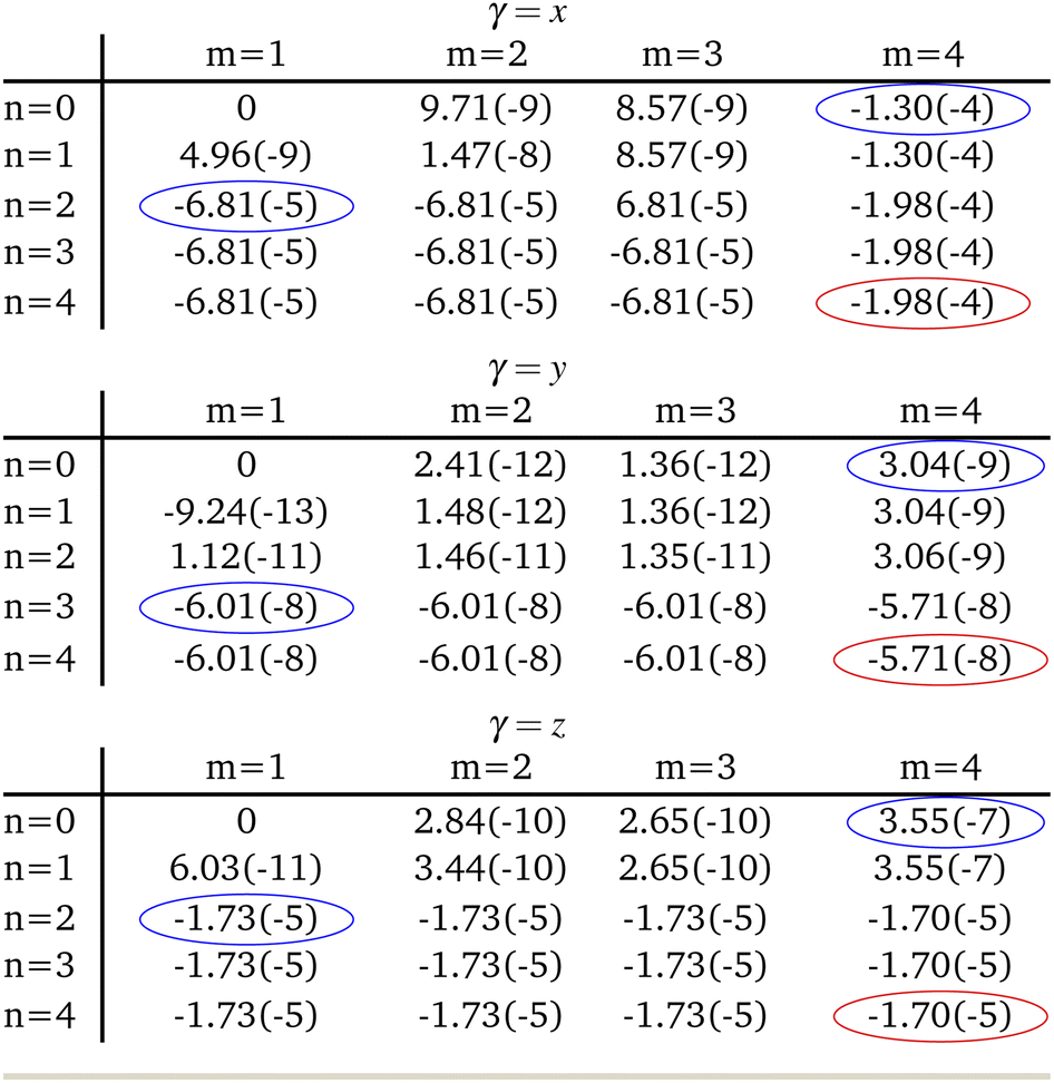
When expanding Mγ across our included 8 states, x, y, and z Cartesian components of −1.98 × 10⁻⁴ au, −5.71 × 10⁻⁸ au, and −1.70 × 10⁻⁵ au were computed respectively, yielding a total moment of 1.99 × 10⁻⁴ au. These components are circled in red in Table 2. It is interesting to note that important contributions to each matrix element come from three states in particular: the fourth triplet excited state, and the second and third singlet excited states. Examination of the photophysical properties for each of these three states shows them to possess the only sizeable transition dipole moments or spin–orbit couplings to other states. In fact, the only large transition dipole components found were 0.71 au for the x component of the first singlet excited state, and 1.27 au for the z component of the second singlet excited state for singlet transition dipole moments, and −0.68 au for the x component of the second triplet excited state. Of all other components, only 5 others from a possible 18 were larger than 0.1 au. Spin–orbit coupling terms were in general much weaker, with only 2 components across a possible 27 being larger than 1 cm−1. Both these couplings were x components, for the second singlet and fourth triplet excited states, with couplings of −15.44 cm−1 and 19.05 cm−1 respectively.
 |
The second order corrected phosphorescent emission profile is shown in Fig. 3. The peak maximum can be found at around 0.65 eV, and extends all the way down to 1.5 eV before tapering off. At 1.4 eV, a very minor peak at the head of the bandshape can clearly be observed. Examination of the normal mode differences between electronic states shows three vibrational normal modes with Huang–Rhys factors larger than 0.5, indicative of very strong spectral features.31,80 Interestingly, the 10 normal modes with the largest Huang–Rhys factors are all between 400–2000 cm−1. Broadening over these peaks would certainly result in a strong bandshape, which is what is observed.
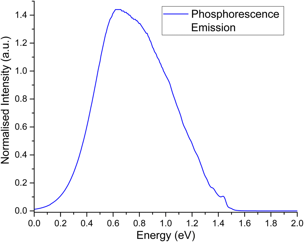 | ||
| Fig. 3 Second order corrected phosphorescence emission spectra predicted from first principles for acridine in the gas phase. | ||
Spectra measured by Morawski & Prochorow11 shows two peaks measured within a dimethyl naphthalene crystalline matrix, as opposed to the single peak in this work. Considering the fact that they also note the phosphorescent spectra to be unexpectedly strong, it may be that the crystalline medium couples very strongly to acridine, which is why two peaks are observed instead of just one. A similar effect can be seen for acridine in 1![[thin space (1/6-em)]](https://www.rsc.org/images/entities/char_2009.gif) :1 ethanol–methanol,46 and a neon matrix.44 The latter case is very interesting, as noble gas matrices have been used to emulate the gas phase such as interstellar conditions.81,82 However, while neon matrices and gas phase studies do yield very similar results,83 they are by definition different, such as how they treat vibrational properties.84 As such, any comparison between the two mediums should be treated with some scepticism.
:1 ethanol–methanol,46 and a neon matrix.44 The latter case is very interesting, as noble gas matrices have been used to emulate the gas phase such as interstellar conditions.81,82 However, while neon matrices and gas phase studies do yield very similar results,83 they are by definition different, such as how they treat vibrational properties.84 As such, any comparison between the two mediums should be treated with some scepticism.
While the phosphorescence bandshape is relatively smooth at room temperature, probing of the computational parameters elude to fine-structured bands. Temperature changes shown in Fig. 4A show the small peak at the head of the band to display a large degree of oscillation, similarly shown for small broadening functions as per Fig. 4B. These fine-structures are due to butterfly-type normal modes around 0.1 eV, breathing-line normal modes around 0.2 eV, and both of their high intensities, as per the infra-ref spectra in Fig. 4C. Conversely, oscillations along the spectral spine are due to deformations of the acridine core.
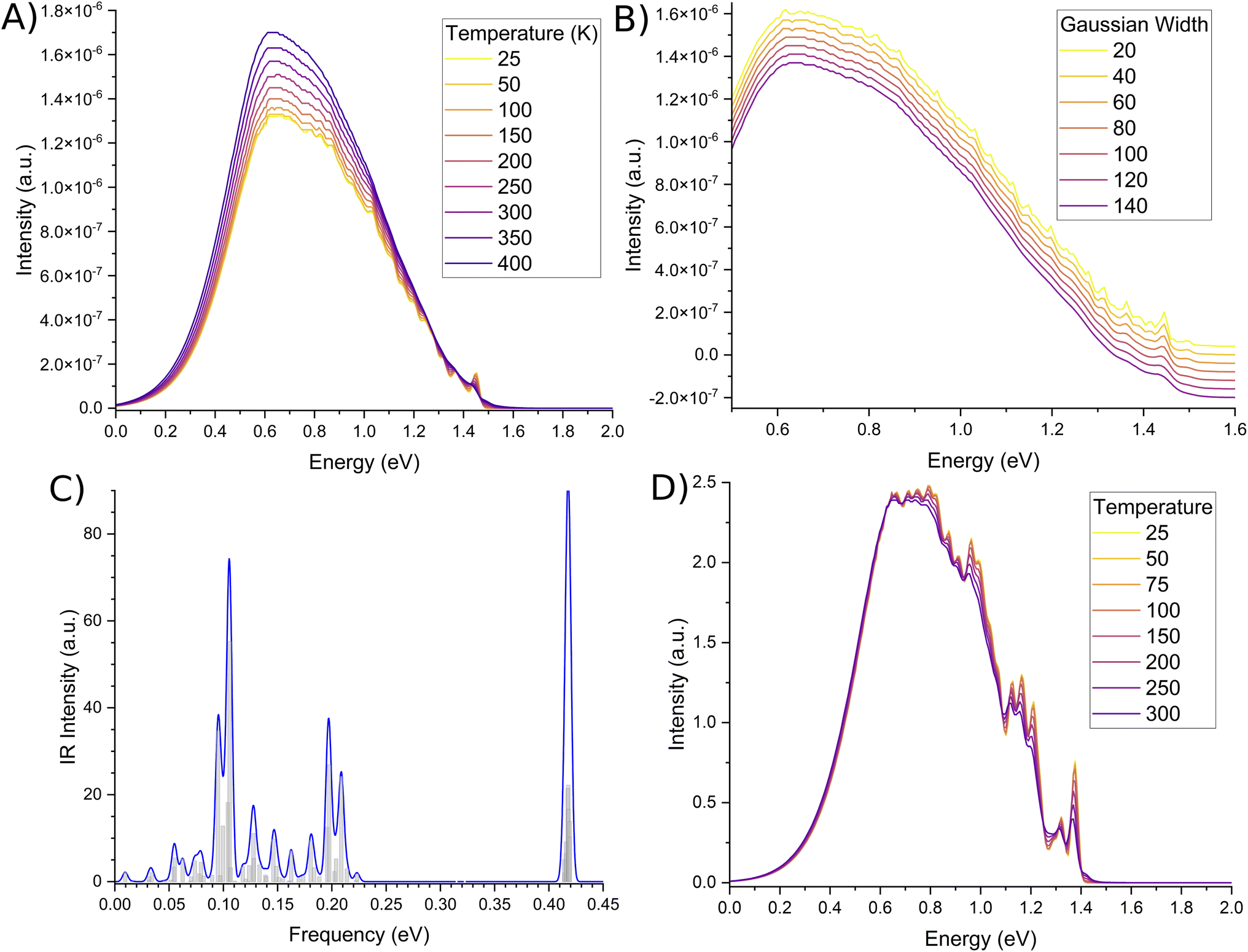 | ||
| Fig. 4 Fine-structure of the phosphorescence spectra. Second-order corrected spectra as a function of (A) temperature, and (B) Gaussian damping, in units of K and cm−1 respectively. Gaussian damping spectra have been offset to more clearly show the minute differences in the fine-structure. (C) Infra-red spectra of the T1 state, with a Gaussian broadening of 4.5 meV. (D) Phosphorescence due to only Franck–Condon terms are shown to illustrate possible convolution of modes resulting in an almost Gaussian lineshape. Spectra are not normalised. | ||
We also note that our emission peak is underestimated with respect to experiment. Based on the fine-structure of our spectra, we are confident this is due to some issue with the CASSCF optimised geometry. This becomes more clear when you examine the phosphorescence spectra calculated using different temperatures for only the Franck–Condon component, as per Fig. 4D. Here the spine is not-nearly as smooth as the second-order corrected lineshape. In fact, significantly more fine-structure details can be observed. In particular, it can be argued that based on the spectral details, there is at least one intense peak along the continuum that was convoluted and blurred. The CASSCF method was a necessity due to the number of high-lying excited states that needed to be computed. However, every derivative component is non-zero. As such, it may be that some vibrational components are being mis-estimated, leading to a more broadened spectral shape as opposed to two distinct peaks.
Application of eqn (1) within the Franck–Condon regime results in a rate constant of 0.0295 s−1 and a corresponding lifetime of 34 s. However, expansion of the matrix element within the Herzberg-Teller regime results in growth of M from 1.99 × 10⁻⁴ au to 7.79 × 10⁻⁴ au, and yields a second order corrected rate constant 0.402 s−1 and a corresponding lifetime of 2.5 s. This is an overall increase by a factor of ∼4 from the first-order to the second-order corrected transition dipole. Importantly, since eqn (1) is dependant on the square of M, the rate and lifetime are affected by a factor of ∼13. A perfect square relation is not observed due to a slight change in the spectra density as well as the transition dipole moment. While no experimental rate or lifetime could be found for the acridine core, this corrected lifetime does compare very well with the experimental rate for acridine orange of 0.56 s−1 as reported by Gryczyński and coworkers47 and reasonably well with the experimental rate for acridine yellow of 2.041 s−1 as reported by Fister & Harris.48
If we consider the growth of Mγ as a function of it's dependent variables, we can begin to more clearly understand how to best maximise Mγ. Eqn (2) has three major inputs: transition dipole components coupling Sn to the ground state or Tm to T1, spin–orbit coupling matrix elements between T1 and Sn or Tm to S0, and the energy gap between states of importance. If we consider an arbitrary state, we can plot the growth of Mγ with respect to increasing transition dipole components and inter-state energy.§ As per the density plot shown in Fig. 5, it becomes obvious that Mγ is maximised for larger transition dipole components with smaller energy gaps. While stronger quantum chemical coupling resulting in larger contributions to Mγ is obvious, it is surprising to see just how fast Mγ increases with respect to the spin–orbit coupling matrix element and inter-state energy. In fact, we see that Mγ is significantly more sensitive to spin–orbit coupling elements than it is to transition dipoles. Where the growth of Mγ with respect to μ could maximise at a value of 0.06 au for a state with a very strong transition dipole of 4–4.5 au, Mγ can gain even more strength with respect to an increasing HSO, whereby even a moderate spin–orbit component of 60 cm−1 can achieve a T1 → S0 transition dipole component of larger than 0.07 au. Should you have a chromophore with significant spin–orbit coupling, like organometallic compounds85 or large conjugated complexes,86 dominating contributions can be larger than 0.15 au for a spin–orbit matrix element of 200 cm−1.
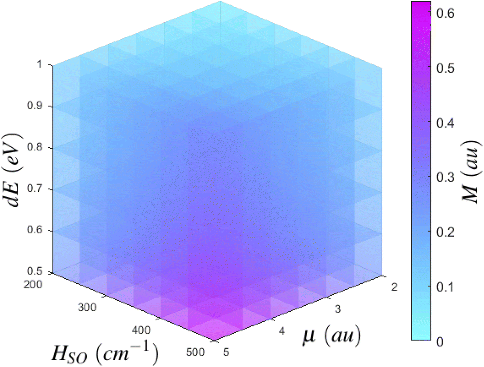 | ||
| Fig. 5 Scaling of M as a function of inter-state couplings. For an arbitrary state, M evolves by increasing either transition dipole matrix elements, spin–orbit coupling matrix element, or the energy separation between states. | ||
In essence, we can therefore claim that while eqn (2) can be expanded to include an infinite number of electronic excited states, only certain states need to be included. Further, which states become important to Mγ could be probed from measurements at the ground state. Computing transition dipole moments for the lowest 30 states show that the 6th singlet and 8th triplet excited states possess large moments of 4.21 au and 2.60 au respectively. However, both of these states display poor spin–orbit coupling to any other state, and as shown in Fig. 5, strong spin–orbit coupling yields larger contributions to Mγ, which is much more important than larger transition dipoles. In fact, the largest spin–orbit coupling component within the 30 lowest states not already included was the  component, with a coupling strength of 13.71 cm−1. However the energy separation would be much too large to yield a significant contribution to Mγ, especially considering how small the spin–orbit coupling component is. As such, it is safe to conclude that we have included most of the important states in our description of phosphorescence in acridine.
With what was just shown, if we were to consider what is required to increase the rate of phosphorescence in any given way, we would be looking to increase the coupling between states. This means larger transition dipole components, larger spin–orbit matrix elements, and smaller energy gaps between electronic states. Larger transition dipole moments are difficult to engineer. Complexation is a common tactic which can drastically alter the photophysics of a compound, for the better with respect to the application. A good example of this is the difference between perylene and perylene diimide, where the former displays a reasonable oscillator strength87 which is increased drastically when compared to perylene diimide.88 One could also consider aggregation, where strong coupling in methanone dimers was shown to increase the phosphorescence lifetime.24 However, of the three quantum chemical properties, the easiest to alter is the strength of spin–orbit coupling. Heavy atoms89,90 or deuteration91–94 have been shown to increase spin–orbit matrix elements. Deuteration in particular has been known to affect the inter-system crossing pathway since the 1960's, with Hutchison & Mangum91 showing how deuteration changes spin-flipping rate constants in rigid gas naphthalene. Both Robinson & Frosch92 and Siebrand93 derived relations highlighting the effects of a change in reduced mass to the Franck–Condon factors and consequential changes in the density of states. However, Bixon & Jortner95 comment on how Siebrand missed the dominant contributions to the matrix element. This effect was demonstrated on azulene whereby an increase to the photoluminescence quantum yield of the second excited state was observed upon deuteration,94 implying a decrease to non-radiative processes. Design of solvatochromic compounds may also be worth considering, as a non-emissive S1 state would give the T1 state a greater chance to be occupied.
5 Conclusion
In this work, we have shown how one can begin from first principles and yield a phosphorescence rate constant, lifetime, and spectral profile. We used gas phase acridine as a case study in order to show how the transition dipole moment for a spin-forbidden transition could be calculated from readily available photophysical properties at the Franck–Condon point. We then discussed how to expand the operator to correct for Herzberg-Teller effects. Using our presented results, we were able to calculate a second order corrected rate constant which agreed very well with the experimental phosphorescent rate for acridine orange, despite the lack of a low-lying nπ* state. Further, we provided evidence that the nπ* state may have been weakly coupled to the first triplet excited state, resulting in a minimal contribution to the phosphorescence transition dipole moment and not necessary in the description of phosphorescent rate constants.We were also able to show that while the operator can be expanded to include any number of electronic excited states, it is only those states which have either reasonably sized spin–orbit matrix element or very large transition dipole components that need to be included, the former being more important than the latter. In justification of this hierarchy of importance, we then explored what would be required to synthetically increase Mγ, highlighting the importance and impact spin–orbit coupling has on the triplet to singlet transition dipole matrix element. From these results, and their discussions, we hope to have made phosphorescence transparent as a quantum chemical process, as well as providing some critical evidence of what is important to exalt the mechanism for photon harvesting applications.
Conflicts of interest
The authors declare no conflicts of interest.Acknowledgements
This work was supported by the Australian Government through the Australian Research Council (ARC) under the Centre of Excellence scheme (project number CE170100026). This work was also supported by computational resources provided by the Australian Government through the National Computational Infrastructure National Facility and the Pawsay Supercomputer Centre. AM would like to thank Rohan J Hudon for helpful discussions with respect to solvent effects.Notes and references
- M. A. El-Sayed, Acc. Chem. Res., 1968, 1, 8–16 CrossRef CAS.
- W. H. Melhuish, Pure Appl. Chem., 1984, 56, 231–245 CrossRef.
- G. Baryshnikov, B. Minaev and H. Ågren, Chem. Rev., 2017, 117, 6500–6537 CrossRef CAS.
- B. Powell, Coord. Chem. Rev., 2015, 295, 46–79 CrossRef CAS.
- S. Nonell and C. Flors, in Comprehensive Series in Photochemical & Photobiological Sciences, Royal Society of Chemistry, 2016, pp. 7–26 Search PubMed.
- Y. Nosaka, T. Daimon, A. Y. Nosaka and Y. Murakami, Phys. Chem. Chem. Phys., 2004, 6, 2917 RSC.
- J. Demas and G. Crosby, J. Mol. Spectrosc., 1968, 26, 72–77 CrossRef CAS.
- F. Zuloaga and M. Kasha, Photochem. Photobiol., 1968, 7, 549–555 CrossRef CAS.
- R. J. Watts and G. A. Crosby, J. Am. Chem. Soc., 1972, 94, 2606–2614 CrossRef CAS.
- D. Baker and G. Crosby, Chem. Phys., 1974, 4, 428–433 CrossRef CAS.
- O. Morawski and J. Prochorow, Chem. Phys. Lett., 1995, 242, 253–258 CrossRef CAS.
- A. S. Polo, M. K. Itokazu and N. Y. M. Iha, Coord. Chem. Rev., 2004, 248, 1343–1361 CrossRef CAS.
- M. Grätzel, Inorg. Chem., 2005, 44, 6841–6851 CrossRef PubMed.
- N. Hoffmann, Chem. Rev., 2008, 108, 1052–1103 CrossRef CAS PubMed.
- S.-C. Lo, C. P. Shipley, R. N. Bera, R. E. Harding, A. R. Cowley, P. L. Burn and I. D. W. Samuel, Chem. Mater., 2006, 18, 5119–5129 CrossRef CAS.
- L. Xiao, Z. Chen, B. Qu, J. Luo, S. Kong, Q. Gong and J. Kido, Adv. Mater., 2010, 23, 926–952 CrossRef PubMed.
- R. C. Evans, P. Douglas and C. J. Winscom, Coord. Chem. Rev., 2006, 250, 2093–2126 CrossRef CAS.
- P.-T. Chou and Y. Chi, Chem.–Eur. J., 2007, 13, 380–395 CrossRef CAS PubMed.
- A. Kapturkiewicz, in Electrochemistry of Functional Supramolecular Systems, John Wiley & Sons, Inc., 2010, pp. 477–522 Search PubMed.
- Q. Zhao, F. Li and C. Huang, Chem. Soc. Rev., 2010, 39, 3007 RSC.
- M. Yu, Q. Zhao, L. Shi, F. Li, Z. Zhou, H. Yang, T. Yi and C. Huang, Chem. Commun., 2008, 2115 RSC.
- Handbook of Porphyrin Science, With Applications to Chemistry, Physics, Materials Science, Engineering, Biology and Medicine - Volume 18: Applications, ed. K. M. S. Karl M Kadish and R. Guilard, World Scientific Pub Co Inc., 2012 Search PubMed.
- H. Kurokawa, H. Ito, M. Inoue, K. Tabata, Y. Sato, K. Yamagata, S. Kizaka-Kondoh, T. Kadonosono, S. Yano, M. Inoue and T. Kamachi, Sci. Rep., 2015, 5, 10657 CrossRef CAS PubMed.
- J. Zhang, E. Sharman, L. Yang, J. Jiang and G. Zhang, J. Phys. Chem. C, 2018, 122, 25796–25803 CrossRef CAS.
- M. Babazadeh, P. L. Burn and D. M. Huang, Phys. Chem. Chem. Phys., 2019, 21, 9740–9746 RSC.
- J. M. Younker and K. D. Dobbs, J. Phys. Chem. C, 2013, 117, 25714–25723 CrossRef CAS.
- R. R. de Haas, R. P. van Gijlswijk, E. B. van der Tol, H. J. Zijlmans, T. Bakker-Schut, J. Bonnet, N. P. Verwoerd and H. J. Tanke, J. Histochem. Cytochem., 1997, 45, 1279–1292 CrossRef CAS PubMed.
- L. Zang, H. Zhao, Y. Zheng, F. Qin, J. Yao, Y. Tian, Z. Zhang and W. Cao, J. Phys. Chem. C, 2015, 119, 28111–28116 CrossRef CAS.
- J. Tatchen and C. M. Marian, Phys. Chem. Chem. Phys., 2006, 8, 2133 RSC.
- K. Mori, T. P. M. Goumans, E. van Lenthe and F. Wang, Phys. Chem. Chem. Phys., 2014, 16, 14523–14530 RSC.
- A. Manian, R. A. Shaw, I. Lyskov, W. Wong and S. P. Russo, J. Chem. Phys., 2021, 155, 054108 CrossRef CAS PubMed.
- A. Manian, F. Campaioli, I. Lyskov, J. H. Cole and S. P. Russo, J. Phys. Chem. C, 2021, 125, 23646–23656 CrossRef CAS.
- D. J. Myers and J. Osteryoung, Anal. Chem., 1973, 45, 381–382 CrossRef.
- J. R. Platt, J. Chem. Phys., 1949, 17, 484–495 CrossRef CAS.
- T. W. Christian Reichardt, Solvents and Solvent Effects in Organic Chemistry, Wiley VCH Verlag GmbH, 2010 Search PubMed.
- A. Marini, A. Muñoz-Losa, A. Biancardi and B. Mennucci, J. Phys. Chem. B, 2010, 114, 17128–17135 CrossRef CAS.
- M. Grzybowski and D. T. Gryko, Adv. Opt. Mater., 2015, 3, 280–320 CrossRef CAS.
- S. J. Bradley, M. Chi, J. M. White, C. R. Hall, L. Goerigk, T. A. Smith and K. P. Ghiggino, Phys. Chem. Chem. Phys., 2021, 23, 9357–9364 RSC.
- A. Manian, R. A. Shaw, I. Lyskov and S. P. Russo, Phys. Chem. Chem. Phys., 2022, 24, 3357–3369 RSC.
- D. Brisker-Klaiman and A. Dreuw, ChemPhysChem, 2015, 16, 1695–1702 CrossRef CAS PubMed.
- L. Serrano-Andrés and B. O. Roos, J. Am. Chem. Soc., 1996, 118, 185–195 CrossRef.
- C. Harthcock, J. Zhang, W. Kong, M. Mitsui and Y. Ohshima, J. Chem. Phys., 2017, 146, 134311 CrossRef PubMed.
- Ò. Rubio-Pons, L. Serrano-Andrés and M. Merchán, J. Phys. Chem. A, 2001, 105, 9664–9673 CrossRef.
- J. Prochorow, B. Kozankiewicz, B. B. D. Gemi and O. Morawski, Acta Phys. Pol., A, 1998, 94, 749–760 CrossRef CAS.
- K. Kikuchi, K. Kasama, A. Kanemoto, K. Ujiie and H. Kikubun, J. Phys. Chem., 1985, 89, 868–871 CrossRef CAS.
- K. Kasama, K. Kikuchi, S. Yamamoto, K. Ujiie, Y. Nishida and H. Kokubun, J. Phys. Chem., 1981, 85, 1291–1296 CrossRef CAS.
- I. Gryczyński, A. Kawski and K. Nowaczyk, J. Photochem., 1983, 21, 81–85 CrossRef.
- J. C. Fister and J. M. Harris, Anal. Chem., 1996, 68, 639–646 CrossRef CAS.
- I. Lyskov, M. Etinski, C. M. Marian and S. P. Russo, J. Mater. Chem. C, 2018, 6, 6860–6868 RSC.
- S. Banerjee, A. Baiardi, J. Bloino and V. Barone, J. Chem. Theory Comput., 2016, 12, 774–786 CrossRef CAS PubMed.
- B. Minaev, G. Baryshnikov and H. Agren, Phys. Chem. Chem. Phys., 2014, 16, 1719–1758 RSC.
- E. Jansson, B. Minaev, S. Schrader and H. Ågren, Chem. Phys., 2007, 333, 157–167 CrossRef CAS.
- J. Franck and E. G. Dymond, Trans. Faraday Soc., 1926, 21, 536 RSC.
- E. Condon, Phys. Rev., 1926, 28, 1182–1201 CrossRef CAS.
- E. U. Condon, Phys. Rev., 1928, 32, 858–872 CrossRef CAS.
- G. Herzberg and E. Teller, Zur Phys. Chem., 1933, 21, 410–446 CrossRef.
- S. K. Lower and M. A. El-Sayed, Chem. Rev., 1966, 66, 199–241 CrossRef CAS.
- A. Schäfer, H. Horn and R. Ahlrichs, J. Chem. Phys., 1992, 97, 2571–2577 CrossRef.
- F. Weigend and R. Ahlrichs, Phys. Chem. Chem. Phys., 2005, 7, 3297 RSC.
- H.-J. Werner, P. J. Knowles, G. Knizia, F. R. Manby, M. Schütz, P. Celani, W. Györffy, D. Kats, T. Korona, R. Lindh, A. Mitrushenkov, G. Rauhut, K. R. Shamasundar, T. B. Adler, R. D. Amos, A. Bernhardsson, A. Berning, D. L. Cooper, M. J. O. Deegan, A. J. Dobbyn, F. Eckert, E. Goll, C. Hampel, A. Hesselmann, G. Hetzer, T. Hrenar, G. Jansen, C. Köppl, Y. Liu, A. W. Lloyd, R. A. Mata, A. J. May, S. J. McNicholas, W. Meyer, M. E. Mura, A. Nicklass, D. P. O'Neill, P. Palmieri, D. Peng, K. Pflüger, R. Pitzer, M. Reiher, T. Shiozaki, H. Stoll, A. J. Stone, R. Tarroni, T. Thorsteinsson and M. Wang, MOLPRO, version 2015.1, a package of ab initio programs, 2015.
- C. Angeli, R. Cimiraglia, S. Evangelisti, T. Leininger and J.-P. Malrieu, J. Chem. Phys., 2001, 114, 10252–10264 CrossRef CAS.
- C. Angeli, R. Cimiraglia and J.-P. Malrieu, Chem. Phys. Lett., 2001, 350, 297–305 CrossRef CAS.
- C. Angeli, R. Cimiraglia and J.-P. Malrieu, J. Chem. Phys., 2002, 117, 9138–9153 CrossRef CAS.
- C. Angeli, M. Pastore and R. Cimiraglia, Theor. Chem. Acc., 2006, 117, 743–754 Search PubMed.
- F. Neese, WIREs Computational Molecular Science, 2011, 2, 73–78 Search PubMed.
- A. Schäfer, C. Huber and R. Ahlrichs, J. Chem. Phys., 1994, 100, 5829–5835 CrossRef.
- S. Grimme and M. Waletzke, J. Chem. Phys., 1999, 111, 5645–5655 CrossRef CAS.
- I. Lyskov, M. Kleinschmidt and C. M. Marian, J. Chem. Phys., 2016, 144, 034104 CrossRef PubMed.
- A. D. Becke, Phys. Rev. A, 1988, 38, 3098–3100 CrossRef CAS.
- U. of Karlsruhe, TURBOMOLE V7.3 2018, a development of University of Karlsruhe and Forschungszentrum Karlsruhe GmbH, TURBOMOLE GmbH, since 2007, 1989–2007, accessed on 1/1/2020, http://www.turbomole.com.
- M. Kleinschmidt, J. Tatchen and C. M. Marian, J. Comput. Chem., 2002, 23, 824–833 CrossRef CAS.
- M. Kleinschmidt and C. M. Marian, Chem. Phys., 2005, 311, 71–79 CrossRef CAS.
- M. Kleinschmidt, J. Tatchen and C. M. Marian, J. Chem. Phys., 2006, 124, 124101 CrossRef PubMed.
- M. Etinski, J. Tatchen and C. M. Marian, J. Chem. Phys., 2011, 134, 154105 CrossRef.
- A. Manian, R. A. Shaw, I. Lyskov and S. P. Russo, J. Chem. Theory Comput., 2022, 1838–1848 CrossRef PubMed.
- L. G. Franca, Y. Long, C. Li, A. Danos and A. Monkman, J. Phys. Chem. Lett., 2021, 12, 1490–1500 CrossRef CAS PubMed.
- D. L. Narva and D. S. McClure, Chem. Phys., 1981, 56, 167–180 CrossRef CAS.
- K. Ishii, M. Kinoshita and H. Kuroda, Bull. Chem. Soc. Jpn., 1973, 46, 3385–3391 CrossRef CAS.
- R. E. C. D. L. G. Trigg, AIP Physics Desk Reference, Springer Nature, 2003 Search PubMed.
- K. Huang and A. Rhys, Proc. R. Soc. London, Ser. A, 1950, 204, 406–423 CAS.
- T. M. Halasinski, D. M. Hudgins, F. Salama, L. J. Allamandola and T. Bally, J. Phys. Chem. A, 2000, 104, 7484–7491 CrossRef CAS.
- J. Szczepanski, C. Wehlburg and M. Vala, Chem. Phys. Lett., 1995, 232, 221–228 CrossRef CAS.
- M. E. Jacox, J. Mol. Struct., 1987, 157, 43–59 CrossRef CAS.
- J. Kalinowski, R. B. Gerber, M. Räsänen, A. Lignell and L. Khriachtchev, J. Chem. Phys., 2014, 140, 094303 CrossRef PubMed.
- A. J. Browne, A. Krajewska and A. S. Gibbs, J. Mater. Chem. C, 2021, 9, 11640–11654 RSC.
- S. Cekli, R. W. Winkel, E. Alarousu, O. F. Mohammed and K. S. Schanze, Chem. Sci., 2016, 7, 3621–3631 RSC.
- T. M. Halasinski, J. L. Weisman, R. Ruiterkamp, T. J. Lee, F. Salama and M. Head-Gordon, J. Phys. Chem. A, 2003, 107, 3660–3669 CrossRef CAS.
- N. Meftahi, A. Manian, A. J. Christofferson, I. Lyskov and S. P. Russo, J. Chem. Phys., 2020, 153, 064108 CrossRef CAS PubMed.
- W. Yang, J. Zhao, C. Sonn, D. Escudero, A. Karatay, H. G. Yaglioglu, B. Küçüköz, M. Hayvali, C. Li and D. Jacquemin, J. Phys. Chem. C, 2016, 120, 10162–10175 CrossRef CAS.
- D. Sasikumar, A. T. John, J. Sunny and M. Hariharan, Chem. Soc. Rev., 2020, 49, 6122–6140 RSC.
- C. A. Hutchison and B. W. Mangum, J. Chem. Phys., 1960, 32, 1261–1262 CrossRef.
- G. W. Robinson and R. P. Frosch, J. Chem. Phys., 1962, 37, 1962–1973 CrossRef CAS.
- W. Siebrand, J. Chem. Phys., 1967, 46, 440–447 CrossRef CAS.
- G. Johnson, L. M. Logan and I. G. Ross, J. Mol. Spectrosc., 1964, 14, 198–200 CrossRef CAS.
- M. Bixon and J. Jortner, J. Chem. Phys., 1968, 48, 715–726 CrossRef CAS.
Footnotes |
| † Unless otherwise stated, all calculation parameters, such as convergence criteria, are run using the default parameters listed in each respective software platform's manual. |
| ‡ The double excitation notation of HOMO2 is equivalent in form to HOMO, HOMO. |
| § While this may be fairly self evident, we feel it is still worth visualising in order to clearly show how Mγ is affected by each of these three quantum chemical parameters. |
| This journal is © The Royal Society of Chemistry 2022 |