
 Open Access Article
 This Open Access Article is licensed under a Creative Commons Attribution-Non Commercial 3.0 Unported Licence
AC conductivity and phase transition of the BST–BFO ceramic doped with Yb
M. Ben Abdessalem *a,
S. Chkoundalia,
A. Oueslatib and
A. Aydia
*a,
S. Chkoundalia,
A. Oueslatib and
A. Aydia
aLaboratory of Multifunctional Materials and Applications (LaMMA), LR16ES18, Faculty of Sciences, University of Sfax, B. P. 1171, 3000 Sfax, Tunisia. E-mail: ben.abdessalem.manel@gmail.com
bCondensed Matter Laboratory, Faculty of Sciences, University of Sfax, B. P. 1171, 3000 Sfax, Tunisia
First published on 26th September 2022
Abstract
The homogeneity of the 0.8(Ba0.8Sr0.2)TiO3–0.2(Bi0.85Yb0.15)FeO3 ceramic, prepared by a solid-state process, was studied and quantitatively analyzed by scanning electron microscopy (SEM) and energy dispersive X-ray spectroscopy (EDX). At ambient temperature, X-ray diffraction shows the existence of only one perovskite phase in the tetragonal structure with the space group P4mm. The thermal variations of  (real part of the dielectric permittivity) for this composition show extended peaks with temperature; this broadening of the peaks can be attributed to the diffuse character of the transition. As the frequency increases, Tm (temperature of maximum permittivity) moves at higher temperatures, and the maximum values of
  decrease. Moreover, the impedance spectra (−Z′′ vs. Z′) show the presence of two arcs of circles that have been modeled with an equivalent electrical circuit. The arcs of the circles centered under the real axis (Z) prove the Cole–Cole-type behavior. Each circle is associated with either the grain effect or grain boundaries. Electrical modulus analysis shows that the capacitance of the ceramic is enhanced, which is in good agreement with the results of complex impedance analysis. The AC conductivity complies with the universal power law. It disputes the modification of AC conductivity by adopting the Arrhenius-type of electrical conductivity. The temperature dependence of alternating current conductivity (σg) and direct current conductivity (σDC) confirms the existence of the ferroelectric–paraelectric phase transition.
1. Introduction
Ferroelectric materials are very interesting due to their simple crystalline structure. They are widely used in electronics, microelectronics and electromechanical transducers1,2 due to their piezoelectric, dielectric and thermoelectric properties.3,4The physical properties of the ferroelectric material Ba0.8Sr0.2TiO3 (BST) confer an increase in its dielectric constant of about 12![[thin space (1/6-em)]](https://www.rsc.org/images/entities/char_2009.gif) 000 and a transition temperature TC of 340 K.5,6 BiFeO3 (BFO) is a multiferroic material that exhibits both ferroelectric and antiferromagnetic orders. Its structure is a rhombohedral distorted perovskite (space group R3c)7 described by a rising Curie temperature (TC = 1103 K) and an antiferromagnetic Neel temperature (TN = 643 K (ref. 8)) and a spin that has been spiral modulated.9,10 In order to promote the properties of the BFO compound and reduce its defects, i.e. extreme current losses and high coercive fields,10 various tests have been effective, including the ion substitution test.
000 and a transition temperature TC of 340 K.5,6 BiFeO3 (BFO) is a multiferroic material that exhibits both ferroelectric and antiferromagnetic orders. Its structure is a rhombohedral distorted perovskite (space group R3c)7 described by a rising Curie temperature (TC = 1103 K) and an antiferromagnetic Neel temperature (TN = 643 K (ref. 8)) and a spin that has been spiral modulated.9,10 In order to promote the properties of the BFO compound and reduce its defects, i.e. extreme current losses and high coercive fields,10 various tests have been effective, including the ion substitution test.
It has been observed in the literature that partial substitution in BFO-based ceramics by rare earths such as La,11 Pr,12 Nd,13,14 Gd,15 Dy16 and Ho17 at the Bi site cause a structural modification and improve the ferroelectric and ferromagnetic properties of the substituted materials. Indeed, the conductivity, ferroelectricity and magnetization are well improved, which makes the obtained compounds more useful in storage applications. In addition, Ilic et al.18 proved that yttrium upgrades the electric and magnetic properties.
In this paper, the main objective of our research work is to study the preliminary structural and electrical properties of BFO by ytterbium (Yb) doping in order to obtain information on the selection of materials for certain significant applications. Similarly, for this reason, we synthesized the compound 0.8(Ba0.8Sr0.2)TiO3–0.2(Bi0.85Yb0.15)FeO3 (BST–BiYbFO) by the solid-state method. This compound was characterized by scanning electron microscopy (SEM), energy dispersive X-ray spectroscopy (EDX) and complex impedance spectroscopy.
2. Experimental
Polycrystalline samples of (BST–BiYbFO) were prepared by adopting the classic solid-state reaction. The starting reagents BaCO3, SrCO3, Bi2O3, TiO2, Fe2O3 and Yb2O3 were of high purity (up to 99.9% purity, Aldrich).These precursors were ground in a planetary mill for 2 hours (h) in ethanol to homogenize the solution and reduce the particle size; the powders obtained were calcined at 770 °C for 3 h. The resulting solution was ground again and pelleted under 3 ton per cm2 and finally sintered at 970 °C for 3 h.
At room temperature (RT), X-ray diffraction (XRD) patterns were obtained on a Siemens D5000 diffractometer using Cu K emission = 1.5460 Å in the angular range of 10° < 2θ < 80° with 10 s for each step of 0.02° around the structure to determine the composition. The FullProf19–21 software was used to analyze the XRD profiles. The morphologies and sizes of the samples were studied directly with a Hitachi SU70 Merlin SEM at an acceleration voltage of 3 kV, equipped with an EDXS energy-dispersive X-ray spectrometer, which was used for the elemental analysis of the different phases. For electrical measurements, the BST–BiYbFO powder was pressed into disks about 8 mm in diameter and 1 mm thick. The electrical properties were measured by an impedance analyzer (TEGAM 3550) in the temperature and frequency ranges of 473–753 K and 100 Hz–2 MHz, respectively.
3. Results and discussion
3.1. X-ray, SEM and EDX characterization
Fig. 1 shows the XRD pattern of the compound BST–BiYbFO recorded at RT. The peaks were successfully indexed using the FullProf program in the tetragonal system with the space group P4mm. The parameters were a = b = 3.9737 Å, c = 3.9840 Å, α = β = γ = 90° and V = 62.9085 Å3, with a reliability factor of χi2 = 2.91, which is consistent with the literature.22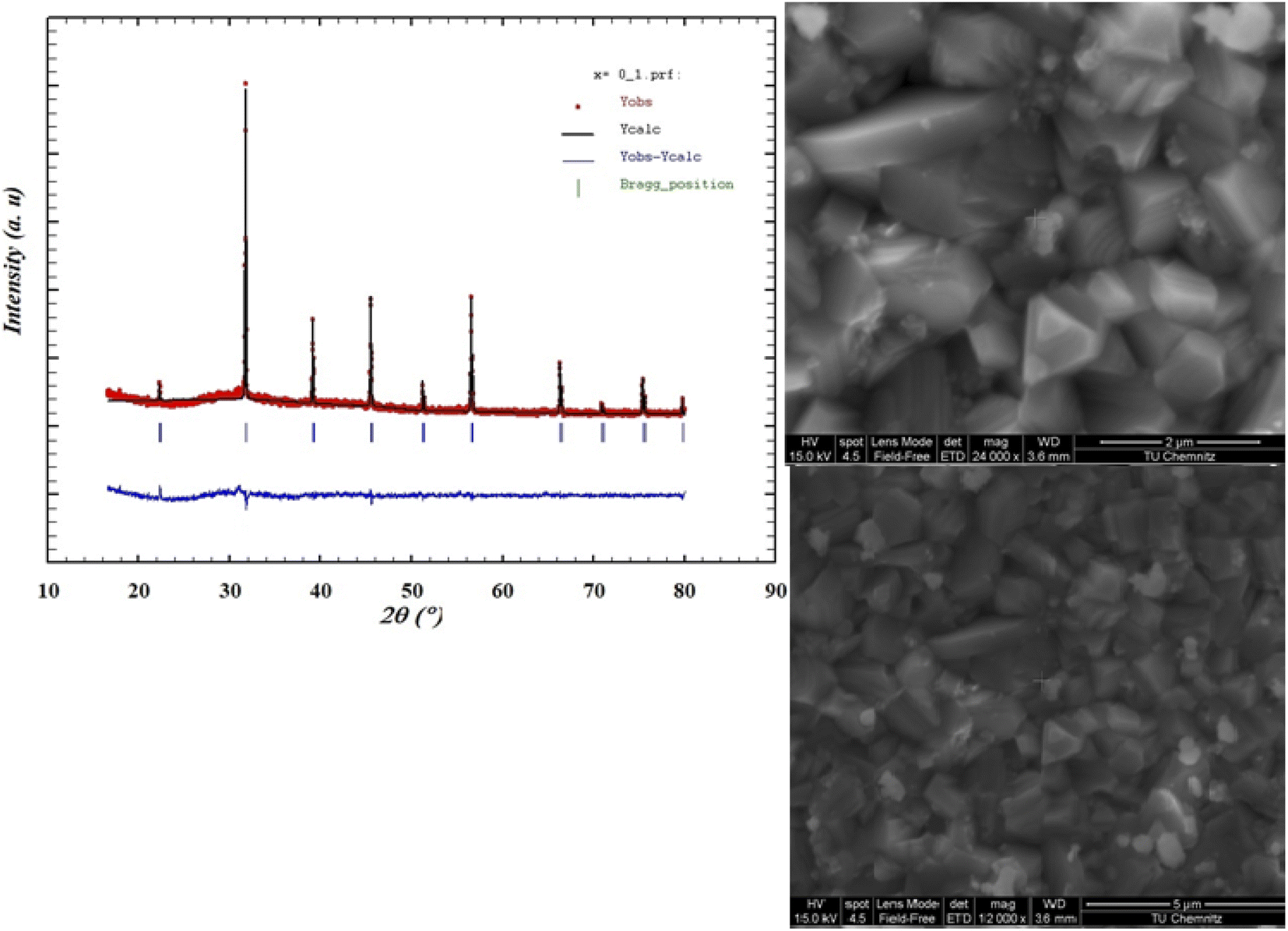 | ||
| Fig. 1 XRD pattern for the tetragonal ceramic 0.8(Ba0.8Sr0.2)TiO3–0.2(Bi0.85Yb0.15)FeO3 at room temperature and SEM micrographs of the ceramic surface. | ||
Analysis of the synthesized powders by XRD and SEM allows us to control the formation of the desired phase and the solid solution boundaries.23 These additional studies can distinguish the elements or phases present in our compound through the detection of backscattered electrons. From the SEM micrographs in Fig. 1 (with a resolution of 2 μm (top) and 5 μm (bottom)), it can be seen that the sample consists of uniform grains with a dimension of about 3.5 μm. It is also observed that the grains are compactly distributed over the surface with some porosity present.
The corresponding EDX24 analysis confirms that all elements are present in the material (Table 1), as indicated in Fig. 2. In addition to the presence of Ba, Sr, Bi, Fe and O, the spectra clearly show the successful Yb doping in BST–BFO. No other impurities were found in the EDX analysis, confirming the clarity of the sample.
| Elements | Weight % | Atomic % |
|---|---|---|
| O | 19.79 | 54.99 |
| Ti | 26.17 | 24.3 |
| Fe | 5.03 | 4 |
| Sr | 7.57 | 3.84 |
| Ba | 35.56 | 11.51 |
| Yb | 4.54 | 1.17 |
| Bi | 0.9 | 0.19 |
| Total | 99.56 | 100 |
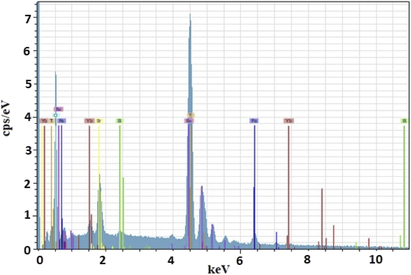 | ||
| Fig. 2 The EDAX spectrum of the 0.8(Ba0.8Sr0.2)TiO3–0.2(Bi0.85Yb0.15)FeO3 ceramic. | ||
3.2. Dielectric study
Investigation of the dielectric allows for the determination of the ferroelectric phase transition temperature and the nature of the relaxing ferroelectric behavior of BST–BiYbFO.Fig. 3(a) shows the variation of the real component of the dielectric permittivity  with frequency. As the frequency increases,
  continues to decrease. For high temperatures, i.e. at 693 K,
  is about 6200 at 125 Hz and then becomes more or less stabilized down to above 10 MHz. The maximum value of
  changes with frequency, leading to a dispersion effect. Two plateaus are observed, with one occurring in the lower-frequency region (102–104 Hz) and another in the higher-frequency region (104–106 Hz) for all the measured temperatures. For electronic ceramics, both grains and grain boundaries provide non-ignorable effects on the electrical properties.
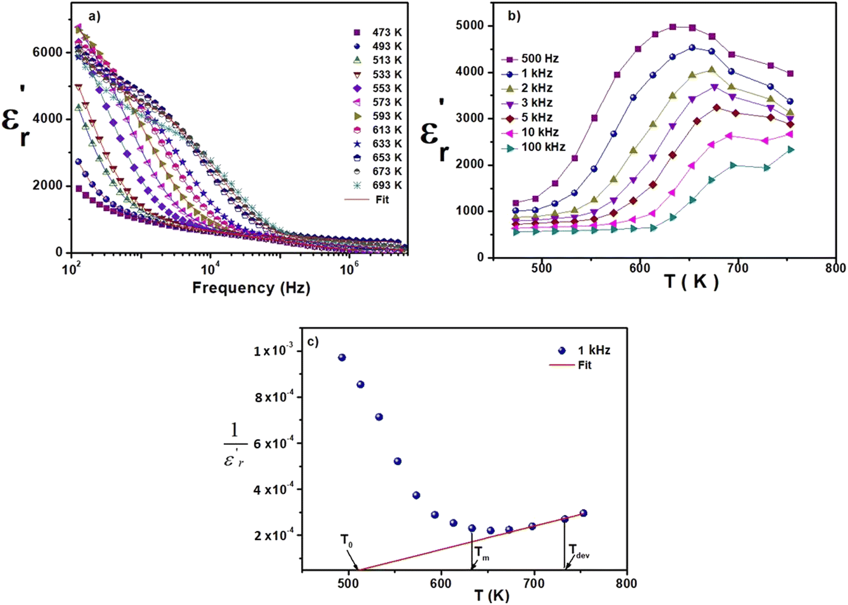 | ||
Fig. 3 (a) Frequency variation of the dielectric constant  at different temperatures. (b) Temperature dependence of the permittivity at different temperatures. (b) Temperature dependence of the permittivity  for BST–BFO. (c) The variation of for BST–BFO. (c) The variation of  versus temperature for the 0.8(Ba0.8Sr0.2)TiO3–0.2(Bi0.85Yb0.15)FeO3 ceramic. versus temperature for the 0.8(Ba0.8Sr0.2)TiO3–0.2(Bi0.85Yb0.15)FeO3 ceramic. | ||
In fact, at lower frequencies, the pattern can be attributed to various types of polarizations in which the space charges are able to follow the frequency of the applied field given that they have enough time. These space charges are generally concentrated in the grain boundaries. On the contrary, at higher frequencies, these space charges do not have sufficient time to undergo relaxation;25,26 it is the effect of the grains that intervenes in this case. High values of dielectric permittivity are observed only at high temperatures and very low frequencies, which may be due to the free charge build-up at interfaces within the bulk of the sample (interfacial Maxwell–Wagner polarization)27 and the interface between the sample and the electrodes (space charge polarization). These results are similar to those found by Patil et al.28
Fig. 3(b), showing the temperature (T) dependence of the real part of the dielectric constant  at different frequencies, proves the existence of a plateau at low temperatures, which can be described as a grain or bulk response of the LBFO compound. As the frequency increases, Tm (the temperature of the maximum value of permittivity) moves toward high temperatures and the maximum values of
  decrease. In addition, a large scatter in the evolution of
  under Tm was observed. This behavior shows the relaxing character of this material. The value of
  increases with temperature to a certain degree and shows a broad dielectric extreme at a certain temperature, Tm = 633 K, which is attributed to the phase transition from an antiferroelectric to a paraelectric state.29–34
The thermal variation of  for this compound, presented in Fig. 3(c), shows a deviation from the Curie–Weiss law given by the equation:35
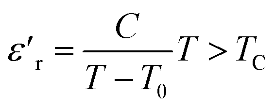
Further theoretical fitting shows that in this case, the transition is diffuse and that the behavior is of the relaxor type. This is a second-order transition, where C is the Curie–Weiss constant and T0 is the Curie–Weiss temperature. Since ion diffusion occurs with increasing temperature, the movement of TC (i.e. the transition from the antiferroelectric to the paraelectric state) at high temperatures is most likely due to space charge polarization.36–39
3.3. Impedance analysis
The behavior of the impedance spectra for different materials is often explained using Argand diagrams (Cole–Cole or Nyquist). In fact, these diagrams are particularly useful for materials that represent one or more relaxation processes, are better separated, and are comparable considering the functional forms of Debye or Cole–Cole.40–45Fig. 4(a) presents the Nyquist diagrams (−Z′′ = f(Z′)) for BST–BiYbFO for different temperatures (473–753 K). The experimental points of these curves are based on circular arcs that pass near the origin and have their centers below the real axis. Since the Debye plots produce semicircles centered on the real axis, this shows that the behavior of this material follows the Cole–Cole model. Any increase in temperature is accompanied by a decrease in resistance, which shows the thermal activation of the conductivity of the material. We examined the thermal evolution of the impedance plots of the BST–BiYbFO compound to verify the assignment of the grain boundaries to the high-temperature dielectric anomaly. With increasing temperature (Fig. 4(b)), the positions of the different frequencies shift from the grain semicircle (higher frequencies) to the grain boundary semicircle (lower frequencies). The anomaly observed at high temperatures could therefore be related to the oxygen vacancies present at the grain boundaries.46–49 By modeling the impedance spectra, a resistive effect of the grain boundaries greater than that of the reinforcements could be demonstrated. This confirms that this dielectric anomaly is mainly due to the oxygen vacancies associated with the grain boundaries. In order to explain the electrical behavior of the material, we prepared an equivalent circuit (inset in Fig. 4(b)) formed from a series of combinations of grains (g) and grain boundaries (gb).
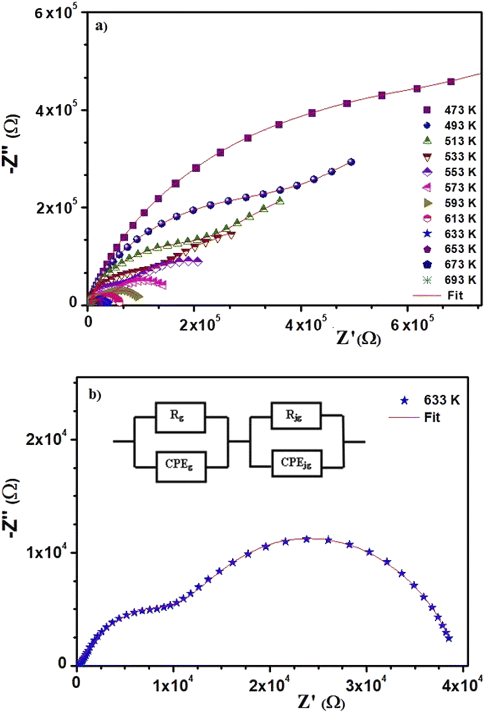 | ||
| Fig. 4 (a) Complex impedance plot at different temperatures of 0.8(Ba0.8Sr0.2)TiO3–0.2(Bi0.85Yb0.15)FeO3. (b) Impedance diagrams at 633 K. | ||
The first consists of a parallel combination of resistance (Rg) and fractal capacitance (CPEg) with the impedance ZCPE = Q(iω)−α (ref. 41) (where Q is a positive constant and a positive number less than or equal to 1), while the second consists of a parallel combination of resistance (Rgb) and a constant phase element (CPEgb). The values of the fitted parameters extracted from the equivalent circuit model are summarized in Table 2.
| T (K) | Rg (Ω) | CPEg (10−8 F) | αg | Rgb (Ω) | CPEgb (10−9 F) | αgb |
|---|---|---|---|---|---|---|
| 473 | 1726700 |
1.672 | 0.684 | 202770 |
1.67 | 0.9245 |
| 493 | 1343100 |
3.553 | 0.644 | 247100 |
1.807 | 0.904 |
| 513 | 1051200 |
5.193 | 0.6188 | 145570 |
1.719 | 0.897 |
| 533 | 685380 |
7.484 | 0.5762 | 64444 |
0.981 | 0.86 |
| 553 | 407060 |
8.982 | 0.5675 | 35420 |
0.8791 | 0.872 |
| 573 | 52061 |
0.550 | 0.756 | 111340 |
12.038 | 0.901 |
| 593 | 30439 |
0.563 | 0.755 | 70369 |
13.228 | 0.883 |
| 613 | 18796 |
0.726 | 0.732 | 42344 |
1.333 | 0.879 |
| 633 | 16098 |
0.236 | 0.652 | 21802 |
87.510 | 0.869 |
| 653 | 5670 | 0.356 | 0.807 | 15401 |
1.353 | 0.868 |
| 673 | 5125 | 1.810 | 0.716 | 8935 | 11.790 | 0.853 |
| 693 | 3395 | 1.967 | 0.675 | 6254 | 13.146 | 0.843 |
The real and imaginary parts of the complex impedance are expressed by:
|
Z′ = ([Rg + Rg2Qgωαgcos(αgπ/2)]/([1 + RgQgωαgcos(αgπ/2)]2 + [RgQgωαgsin(αgπ/2)]2)) + ([Rgb + Rgb2Qgbωαgbcos(αgbπ/2)]/([1 + RgbQgbωαgbcos(αgbπ/2)]2 + [RgbQgbωαgbsin(αgbπ/2)]2))
| (1) |
|
Z′′ = ([Rg2Qgωαgsin(αgπ/2)]/([1 + RgQgωαgcos(αgπ/2)]2 + [RgQgωαgsin(αgπ/2)]2)) + ([Rgb2Qgbωαgbsin(αgbπ/2)]/([1 + RgbQgbωαgbcos(αgbπ/2)]2 + [RgbQgbωαgbsin(αgbπ/2)]2))
| (2) |
The variation of the real part of the impedance (Z′) as a function of frequency for the BST–BiYbFO composition is plotted in Fig. 5(a) for different temperatures. It can be seen that Z′ decreases with increasing temperature and frequency, leading to an increase in electrical conduction in the sample depending on these parameters. High values of Z′ are obtained at low frequencies and low ones correspond to high frequencies (>106 Hz). This behavior could be explained by the presence of space charges and/or ionic conduction.50–53 At high and medium frequencies, Z′ is independent of temperature, which reduces the influence of space charges.54 In fact, in the highest frequency range, all the curves merge and become independent of frequency, suggesting a possibility of space charge release.53
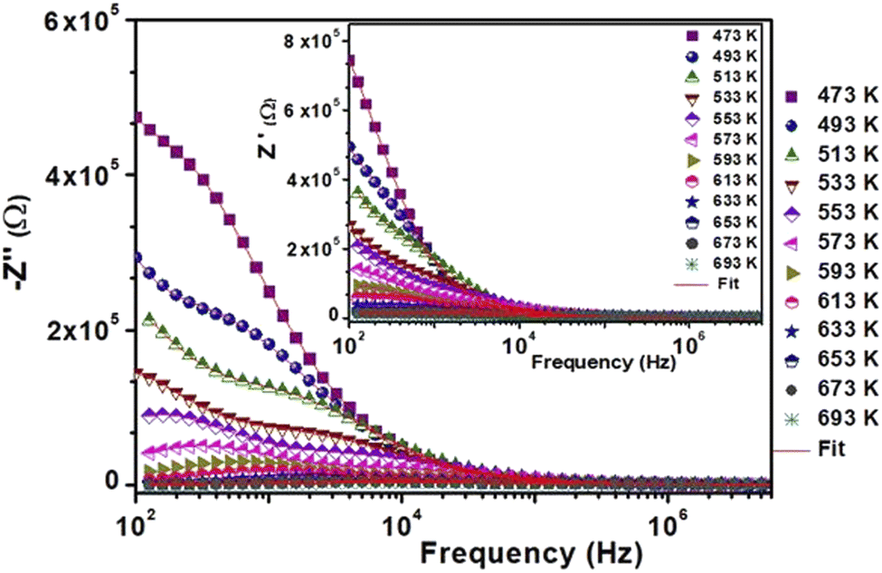 | ||
| Fig. 5 Variation of the real part Z′ and the imaginary part −Z′′ of the impedance as a function of frequency at various temperatures. | ||
Fig. 5(b) shows the change in the imaginary part of the impedance (Z′′) with frequency for the BST–BiYbFO composition at different temperatures. At higher frequencies and higher temperatures, the  peaks change and broaden, indicating relaxation in the studied composition. This curve is useful to evaluate the relaxation frequency in materials with resistive character.55 The asymmetrical broadening of the peak under the influence of temperature suggests a temperature-dependent distribution of relaxation times.56
3.4. AC conductivity studies
Fig. 6 shows the frequency dependence of electrical conductivity (AC) at different temperatures. The conductivity model is represented by two distinct regions. First, the conductivity in the low-frequency range is frequency independent, which characterizes the direct conductivity due to the displacement of the charge carriers.57 Second, the AC conductivity–compatible dispersion regime occurs at a higher frequency.58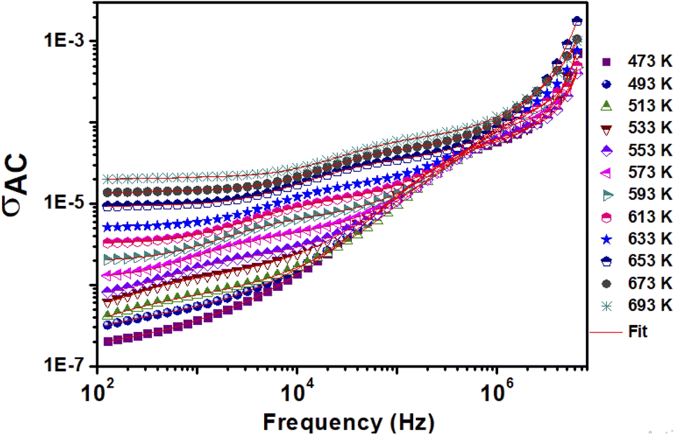 | ||
| Fig. 6 Variation of the AC conductivity (σAC) with frequency at selected temperatures of 0.8(Ba0.8Sr0.2)TiO3–0.2(Bi0.85Yb0.15)FeO3. | ||
Jonscher's law is commonly used to explain the phenomenon of conductivity dispersion:42,59,60
| σAC(ω) = σDC + AωS | (3) |
From these curves, we can see that Jonscher's classical equation (eqn (3)) does not explain the behavior of our experimental data. Using eqn (4) agrees better with the experimental values and the developed equation is called the Jonscher equation.62
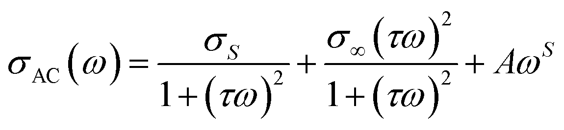 | (4) |
3.5. DC electrical conductivity
Electrical conductivity depends on the slightly bound charged particles that move through a material under the effect of a continuous electric field. The following relationship can be used to calculate electrical conductivity (DC) from resistance (R):
 | (5) |
 | (6) |
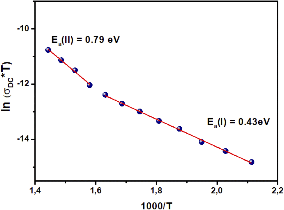 | ||
| Fig. 7 Temperature dependence of ln(σDC × T). | ||
3.6. Modulus
Macedo et al. first developed the modulus formalism in 1972.66 This formalism has been applied to the study of material electrical characteristics. It is used to determine the relaxation times of the conductivity. The complex modulus is expressed as:| M* = jωC0Z = M′ + jM′′ | (7) |
Fig. 8 shows the variation of the imaginary part M′′ of the complex modulus as a function of the real part M′ at different temperatures. The influence of grains and grain boundaries is related to the two observed semicircles, consistent with previous findings.
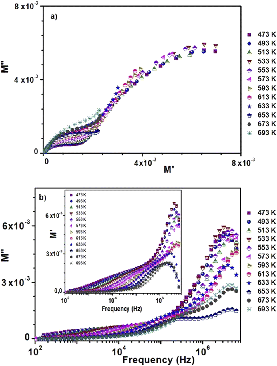 | ||
| Fig. 8 (a) Argand plot of 0.8(Ba0.8Sr0.2)TiO3–0.2(Bi0.85Yb0.15)FeO3. (b) Spectroscopy plots of the M′ and M′′ curves. | ||
Fig. 8(a) shows the change in the real part M′ of the electrical modulus as a function of frequency at different temperatures. It is observed that, at low frequencies, the values of M′ are very low (from 106 Hz). The spectra of M′ present rapid decreases according to the equation: 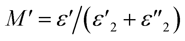 . Moreover, the increase in M′ is due to the accumulation of charges at the electrode–electrolyte interface, i.e. it is space charge polarization.67,68
The fluctuation of the imaginary part M′′ of the electrical modulus as a function of frequency at various temperatures is shown in Fig. 8(b). These fluctuations are found in two temperature ranges: T < 633 K and T > 633 K. This confirms the existence of the two conduction domains. In the first domain, the maxima of the curves are not of the same levels, and in the second domain, the maxima of the curves decrease when the temperature increases. Moreover, these spectra present asymmetrical relaxation peaks whose maxima shift towards high frequencies when the temperature increases.69,70
4. Conclusion
In this study, the interaction of the structure and electrical properties of the BST–BiYbFO ceramic prepared by solid-state technology has been studied.According to X-ray diffraction, the sample shows a tetragonal structure with a space group of P4mm. Dielectric measurement showed a relaxing ferroelectric behavior at the phase transition temperature of 633 K. The analysis of the impedance Z′ as a function of Z′′ shows two semicircles that were modeled by a simple equivalent circuit.
The two relaxation peaks in the modulus spectra represent the input of grains and grain boundaries to the electrical response. With increasing temperature, electrical modulus and impedance measurements showed a relaxing effect shifting to higher frequencies.
For AC conductivity, the law of universal power states that σAC(ω) = σDC + AωS. Activated Arrhenius-type electrical transport mechanisms are responsible for the linear variation in DC conductivity. The frequency-dependent conductivities of the title compound show two distinct linear zones: EI = 0.44 eV in region I (T < TC) and EII = 0.68 eV in region II (T > TC). This shows that the presence of oxygen is the main cause of electrical conduction in BST–BiYbFO.
Conflicts of interest
Authors declare that they have no conflict of interest or personal relationships that could have appeared to influence the work reported in this paper.References
- G. F. Teixeira, T. R. Wright, D. C. Manfroi, E. Longo, J. A. Varela and M. A. Zaghete, Mater. Lett., 2015, 139, 443 CrossRef CAS
.
- M. Ben Abdessalem, S. Aydi, A. Aydi, N. Abdelmoula, Z. Sassi and H. Khemakhem, J.Applied Physics A., 2017, 123, 583 CrossRef
- A. S. Bhalla, R. Guo and R. Roy, Mater. Res. Innovations, 2000, 4, 3 CrossRef CAS
- C. D. Chandler, C. Roger and M. J. H Smith, Chem. Rev., 1993, 93, 1205 CrossRef CAS
- L. BenAbdessalem, M. BenAbdessalem, A. Aydi and Z. Sassi, J. Mater. Sci.: Mater. Electron., 2017, 28, 14264–14270 CrossRef CAS
- H. Abdelkefi, H. Khemakhem, G. Velu, J. C. Carru and R. V. Muhll, J. Alloys Compd., 2005, 399, 1 CrossRef CAS
- S. Kongtaweelert, D. C. Sinclair and S. PanichphantCurr, Appl. Phys., 2006, 6, 474 Search PubMed
- P. Fischer, M. Polomska, I. Sosnowska and M. Szymanshi, J. Phys. C, 1980, 13, 1931–1940 CrossRef CAS
- B. Wodecka-Dus and D. Czekaj, Arch. Metall. Mater., 2011, 56, 1127 CAS
- G. Catalan and J. F. Scott, Adv. Mater., 2009, 21, 2463 CrossRef CAS
- S.-T. Zhang, Y. Zhang and M.-H. Lu, et al., Appl. Phys. Lett., 2006, 88, 3 Search PubMed
- D. Varshney, P. Sharma, S. Satapathy and P. K. Gupta, J. Alloys Compd., 2014, 584, 232–239 CrossRef CAS
- G. L. Yuan, S. W. Or, J. M. Liu and Z. G. Liu, Appl. Phys. Lett., 2006, 89, 052905 CrossRef
- G. L. Yuan and S. W. Or, Appl. Phys. Lett., 2006, 88, 062905 CrossRef
- V. A. Khomchenko, D. A. Kiselev and I. K. Bdikin, et al., Appl. Phys. Lett., 2008, 93, 262905 CrossRef
- V. A. Khomchenko, D. V. Karpinsky and A. L. Kholkin, et al., J. Appl. Phys., 2010, 108, 074109 CrossRef
- N. Jeon, D. Rout, W. Kim and S. L. Kang, Appl. Phys. Lett., 2011, 98, 072901 CrossRef
- N. I. Ilic, J. D. Bobic, B. S. Stojadinovic, A. S. Dzunuzovic, M. M. Vijatovic Petrovic, Z. D. Dohcevic-Mitrovic and B. D. Stojanovic, J. Mater. Res. Bullet., 2016, 77, 60–69 CrossRef CAS
- T. Roismel and J. Rodriguez-Carvajal, CNRS-Université de rennes. Laboratoire Brillouin (CEA-CNRS), version 3.70, May 2004, LLB-LCSIM, 2005 Search PubMed
- M. ben Abdessalem, A. Aydi, Z. Sassi, L. Seveyrat, V. Perrin, N. Abdelmoula, H. Khemakhem and L. Lebrun, J. Appl. Phys., 2021, 127, 80 CrossRef
- H. M. Rietfeld, J. Appl. Crystallogr., 1969, 2, 65–71 CrossRef
- H. Ghoudi, S. Chkoundali, A. Aydi and K. Khirouni, Appl. Phys. A, 2017, 123, 703 CrossRef
- D. A. Samuelson, Energy dispersive X-ray microanalysis, Methods Mol. Biol., 1998, 108, 413–424 CAS
- Z. Mohamed, E. Tka and J. Dhahri, et al., J. Alloys Compd., 2014, 615, 290–297 CrossRef CAS
- J. Liu, X. Q. Liu and X. M. Chen, J. Appl. Phys., 2016, 119, 204102 CrossRef
- H. O. Rodrigues, G. F. M. Pires Junior, J. S. Almeida, E. O. Sancho, A. C. Ferreira, M. A. S. Silva and A. S. B. Sombra, J. Phys. Chem. Solids, 2010, 71, 1329 CrossRef CAS
- X. J. Xi, S. Y. Wang, W. F. Liu, H. J. Wang, F. Guo, X. Wang, J. Gao and D. J. Li, J. Alloys Compd., 2014, 603, 224 CrossRef CAS
- D. R Patil and B. K Chougule, Effect of copper substitution on electrical and magnetic properties of NiFe2O4 ferrite, Mater. Chem. Phys., 2009, 117, 35 CrossRef CAS
- D. R. Patil, S. A. Lokare, R. S. Devan, S. S. Chougule, Y. D. Kolekar and B. K. Chougule, J. Phys. Chem. Solids, 2007, 68, 1522 CrossRef CAS
- H. Ghoudi, S. Chkoundali, Z. Raddaoui and A. Aydi, RSC Adv., 2019, 9, 25358 RSC
- H. Slimi, A. Oueslati and A. Aydi, RSC Adv., 2021, 11, 14504 RSC
- M. Bourguiba, Z. Raddaoui, M. Chafraa and J. Dhahri, RSC Adv., 2019, 9, 42252 RSC
- M. ben Abdessalem, A. Aydi and N. Abdelmoula, J. Alloys Compd., 2019, 774, 685–693 CrossRef
- M. A. Ahmed, S. F. Mansour, S. I. El-Dek and M. MKaramany, J. Rare Earths, 2016, 34, 495 CrossRef CAS
- Y. Chaudhari, C. M. Mahajan, A. Singh, P. Jagtap, R. Chatterjee and S. Bendre, J. Magn. Magn. Mater., 2015, 395, 329 CrossRef CAS
- E. Cai, Q. Liu, S. Zhou, Y. Zhu and A. Xue, J. Alloys Compd., 2017, 726, 1168 CrossRef CAS
- A. Chaudhuri and K. Mandal, Mater. Res. Bull., 2012, 47, 1057 CrossRef CAS
- R. Bellouz, M. Oumezzine, A. Dinia, G. Schmerber, E. l.-K. Hlil and M. Oumezzine, RSC Adv., 2015, 5, 64557–64565 RSC
- Y. K. Jun, W. T. Moon, C. M. Chang, H. S. Kim, H. S. Ryu, J. W. Kim, K. H. Kim and S. H. Hong, Solid State Commun., 2005, 135, 133 CrossRef CAS
- T. S. Irvine, D. C. Sinclair and A. R. West, Adv. Mater., 1990, 2, 132–138 CrossRef
- L. Miladi, A. Oueslati and K. Guidara, RSC Adv., 2016, 6, 83280–83287 RSC
- A. K. Jonscher, Dielectric Relaxation in Solids, Chelesa Dielectric Press, London, 1983 Search PubMed
- P. H. Xiang, Y. Kinemuchi, T. Nagaoka and K. Watari, Mater. Lett., 2005, 59, 3590 CrossRef CAS
- M. ben Abdessalem, A. Aydi and N. Abdelmoula, J. Alloys Compd., 2019, 774, 685–693 CrossRef
- E. Barsoukov and J. R. Macdonald, Impedance Spectroscopy : Theory, Experiment, and Applications, Wiley Interscience, New York, 2nd edn, 2005, p. 14 Search PubMed
- J. B. Jorcin, M. E. Orazem, N. Pebere and B. Tribollet, Electrochim. Acta, 2006, 51, 1473–1479 CrossRef CAS
- R. K. Mishra, D. K. Pradhan, R. N. P. Choudhary and A. Banerjee, J. Phys.: Condens. Matter, 2008, 20, 045218 CrossRef
- A. Ruff, S. Krohns, F. Schrettle, V. Tsurkan, P. Lunkenheimer and A. Loidl, Absence of polar order in LuFe2O4, Eur. Phys. J. B, 2012, 85, 290 CrossRef
- F. S. Howel, R. A. Bose, P. B. Maado and C. T. Moynihan, J. Phys. Chem., 1974, 78, 639–648 CrossRef
- I. Coondoo, N. Panwar, M. A. Rafiq, V. S. Puli, M. N. Rafiq and R. S. Katiyar, Ceram. Int., 2014, 40, 9895–9902 CrossRef CAS
- N. Sdiri, R. Jemai, M. Bejar, M. Hussein, K. Khirouni, E. Dhahri and S. Mazen, Solid State Commun., 2008, 148, 577–581 CrossRef CAS
- J. Suchanicz, Mater. Sci. Eng. B, Solid-State Mater. Adv. Technol, 1998, 55, 114 CrossRef
- M. Tachibana, Solid State Commun., 2015, 221, 33–35 CrossRef CAS
- M. Idrees, M. Nadeem and M. M. Hassan, J. Phys. D: Appl. Phys., 2010, 43, 155401 CrossRef
- M. Younes, M. Nadeem, M. Atif and R. Grossinger, J. Appl. Phys., 2010, 109, 93704 CrossRef
- M. Nadeem and M. J. Akhtar, J. Appl. Phys., 2008, 104, 103713 CrossRef
- S. Brahma, R. N. P. Choudhary and S. A. Shivashankar, J. Phys. Chem. Solids, 2012, 73, 357 CrossRef CAS
- F. Yakuphanoglu, Y. Aydogdu, U. Schatzschneider and E. Rentschler, Solid State Commun., 2003, 128, 63 CrossRef CAS
- A. K. Jonscher and M. S. Frost, Thin Solid Films, 1976, 37(2), 267 CrossRef CAS
- Y. Moualhi, R. M'nassri, H. Rahmouni, M. Gassoumi and K. Khirounic, RSC Adv., 2020, 10, 33868 RSC
- A. K. Jonscher, Nature, 1977, 267, 673 CrossRef CAS
- M. Ben Bechir, K. Karoui, M. Tabellout, K. Guidara and A. Ben Rhaiem, J. Alloys Compd., 2014, 588, 551 CrossRef CAS
- N. F. Mott and E. A. Davis, Electronic Process in Non-crystalline Materials, Clarendon Press, Oxford, 1979 Search PubMed
- P. C. Sati, M. Arora, S. Chauhan, M. Kumar and S. Choker, Ceram. Int., 2014, 40, 7805 CrossRef CAS
- M. M. Costa, G. F. M. Pires-Junior and A. S. B. Sombra Mater, Chem. Phys., 2010, 123, 35 CAS
- P. B. Macedo, C. T. Moynihan and N. L. Laberge, Phys. Chem. Glasses, 1973, 14, 122 Search PubMed
- R. Das and R. N. P. Choudhary, Solid State Sci., 2019, 87, 1–8 CrossRef CAS
- M. M. Costa, G. F. M. Pires, A. J. Terezo, M. P. F. Grac and A. S. B. Sombra, J. Appl. Phys., 2011, 110(1–7), 034107 CrossRef
- C. T. Moynihan, L. P. Boesch and N. L. Laberge, Phys. Chem. Glasses, 1973, 14, 122–125 CAS
- D. C. Sinclair and A. R. West, J. Appl. Phys., 1989, 66, 3850–3856 CrossRef CAS
| This journal is © The Royal Society of Chemistry 2022 |