Density functional theory for the prediction of interfacial properties of molecular fluids within the SAFT-γ coarse-grained approach

Abstract

Recently, we have proposed the SAFT-VR Mie MF DFT approach [Algaba et al., Phys. Chem. Chem. Phys., 2019, 21, 11937–11948] to investigate systems that exhibit fluid–fluid interfaces. This formalism is based on the combination of the Statistical Associating Fluid Theory for attractive potentials of variable range using Mie intermolecular potential (SAFT-VR Mie) and a Density Functional Theory (DFT) treatment of the free energy. A mean-field approach is used to evaluate the attractive term, neglecting the pair correlations associated to attractions. This theory has been combined with reported SAFT-γ Coarse-Grained (CG) Mie force fields to provide an excellent description of the vapor–liquid interface of carbon dioxide and water pure fluids. The present work is a natural and necessary extension of this previous study. We assess the adequacy of the proposed methodology for dealing with inhomogeneous fluid systems of large complex molecules, in particular carbon tetrafluoride and sulfur hexafluoride greenhouse gases, the refrigerant 2,3,3,3-tetrafluoro-1-propene, and the long-chain n-decane and n-eicosane hydrocarbons. The obvious diversity of these fluids, their chemical and industrial interest, and the fact of that SAFT-γ CG Mie force fields have been reported for them justify such choice. With the aim of testing the theory, we perform Molecular Dynamics simulations in the canonical ensemble using the direct coexistence technique for the same models. We focus both on bulk, such as coexistence diagrams and vapor pressure curves, as well as interfacial properties, including surface tension. The comparison of the theoretical predictions with the computational results as well as with experimental data taken from the literature demonstrates the reliability and generalization of this method for dealing simultaneously with vapor–liquid equilibrium and interfacial phenomena. Hence, it appears as a potential tool for the interface analysis, with the main advantage over molecular simulation of low computational cost, and solving the experimental difficulties in accurately measuring the surface tension of certain systems.

---

1 Introduction

Description of the thermodynamics and structure of molecular systems from a theoretical perspective is essential from the practical and fundamental viewpoints. Different techniques and levels of resolution can be used depending on the length and time scales required to compute the desired properties of the targeted substances. Since interfacial phenomena play a main role in a broad range of biological, chemical and industrial processes, to investigate interfacial systems is of particular great interest but challenging due to the inhomogeneous nature.

One of the most sophisticated and successful theoretical treatments to study interfacial phenomena is unquestionably Density Functional Theory (DFT).^1–6 As traditional ab initio methods, DFT is a computational quantum mechanical modelling method and thus involves a high level of resolution. However, this can be avoided if the precise details of the electronic structure do not play a direct role in determining the macroscopic properties of the system at large scales. Following this approximation, standard DFT used routinely in quantum mechanical calculations can be also applied to solve problems in the time and length scales at which dispersive interactions between molecules play a key role and determine the macroscopic behavior of the system. In statistical mechanics, DFT is based on the construction of a free-energy functional that depends on the density of the system, or more precisely, it is a functional that depends explicitly on the position r, i.e., ρ = ρ(r). From this knowledge, it is possible to predict the thermodynamic properties of the target fluid using standard tools from calculus of variations. Several authors have discussed the general approaches for the construction of free-energy functionals and the different approximations that are commonly employed.^1–6 Overall, the free-energy functional is divided in two parts: a reference term that incorporates only the ideal and short-range interactions, and a perturbative term in which the long-range interactions are included. The reference term can be treated by using a local density or a weighted-density approximation.

On the other hand, the increasing computational power as well as the development of more sophisticated force fields and efficient numerical algorithms has made possible to use classical atomistic simulation as a routine technique for the description of the molecular fluids, including systems that exhibit different kinds of inhomogeneities, such as fluid–fluid and solid–fluid interfaces, among many others. Molecular dynamics simulation technique has been widely used to explore the behavior on time scales extending over hundreds and even thousands of nanoseconds.^7,8 The degrees of freedom characterizing the quantum or atomistic models that are not relevant in the large-scale regime can be either ignored or subsumed into effective interactions between bundles of matter (superatoms) formed by combining several atoms or chemical functional groups. Coarse-graining (CG) methodologies are based on this low level of resolution to represent the systems under study, but still retaining an appropriate description of the properties of interest. Then, they are increasingly being used to span the gap between the atomistic and mesoscopic representations of matter. We recommend the excellent review by Müller and Jackson and the references therein.⁹

Other successful formalism for the prediction of thermodynamic properties, and particularly fluid-phase equilibria, is the Statistical Associating Fluid Theory (SAFT)^10,11 The SAFT equation of state (EoS) comprises different contributions that take into account the total free energy of the systems from a rigorous statistical-mechanics viewpoint (in particular perturbation theory). The general form of the SAFT expression of the Helmholtz free energy is based on Wertheim's first-order thermodynamic perturbation theory for associating systems.^12–15 A number of variants of this molecular-based EoS have been developed over the last decades,¹⁶ including SAFT-HS,^17,18 soft-SAFT,^19,20 perturbed-chain SAFT (PC-SAFT),²¹ and the Statistical Associating Fluid Theory for attractive potentials of variable range (SAFT-VR).^22,23 Lafitte et al.²⁴ proposed a new version based on the Mie intermolecular potential (SAFT-VR 2006 Mie), and later, a more sophisticated and accurate theory for molecular chains that interact with the same intermolecular potential, the well-known SAFT-VR Mie formalism.²⁵ This later version is able to provide high precision in the near-critical region, and thus allows one to represent globally the thermodynamic properties and fluid-phase equilibria of pure fluids and their mixtures.

Jackson and co-workers,^9,26–30 combining CG methodologies⁹ and the SAFT-VR Mie approach,²⁵ developed a series of CG models generated using experimental data. These authors have used this formalism to propose new CG models that are able to predict accurately the thermodynamic behaviour of molecular chains.⁹ The resulting family of the CG models for real substances is named generically SAFT-γ CG force fields. These CG force fields using the SAFT-VR Mie EoS was exemplified with the representation of firstly the carbon dioxide,²⁷ and then water²⁹ as single Mie spherical CG segments. Despite their simplicity, these SAFT-γ CG Mie force fields were shown to provide an excellent description of numerous vapor–liquid properties. Molecular simulations employing these simple models takes the advantage of involving significantly lower computational cost compared with using atomistic models. The generic nature of the procedure was demonstrated by the later development of CG force fields for diverse molecular systems.

An efficient approach to study inhomogeneous pure fluids has been the SAFT-VR DFT formalism proposed by Gloor et al.,^31,32 an improved version of the SAFT-HS DFT.^33,34 It is based on the SAFT-VR Helmholtz free energy under a formal DFT treatment, where the different terms of the equation of state are separated in order to describe the short and long-range interactions. This theory has been applied to determine the interfacial properties of a wide variety of fluids, and also it was extended to study binary mixtures.^35,36

In a more recent work,³⁷ we introduced a new theoretical perspective: we extended the general SAFT-VR DFT formalism originally proposed to deal with square-well molecular chains to predict the thermodynamic behaviour of Mie molecular chains. The proposed DFT version, that follows the Helmholtz free energy of the SAFT-VR Mie approach, is based on: (a) a local reference term to deal with the short-range interactions; (b) a perturbation term to take into account the long-range attractive forces; and (c) attractive interactions calculated via a mean-field approximation. Such a constructed methodology takes the potential of SAFT EoS for describing bulk behaviors, and additionally allows to determine interfacial properties such as surface tensions.

This new approach, named SAFT-VR Mie MF DFT, has been assessed by studying chain molecules formed from Mie segments, examining the influence of the molecular chain length as well as of the repulsive exponent of the intermolecular potential. Theoretical predictions were compared with computer simulation data taken from the literature³⁸ for density profiles and surface tension of Mie chain-like molecules, obtaining good agreement throughout the target thermodynamic coexistent conditions, especially for short-chain molecules. Once the accuracy of this version of DFT to predict the interfacial properties of Mie chain-like molecules was demonstrated, it was used to predict the vapor–liquid interfacial properties of real molecules. In particular, the authors focused on carbon dioxide²⁷ and water,²⁹ using the reported SAFT-γ CG force fields for these molecules. The agreement among the theoretical predictions, MD simulation results and the available experimental data was found excellent, in particular for carbon dioxide, and even for the surface tension, which is a very sensitive property to molecular details. Thus, this theoretical framework combined with SAFT-γ CG force fields appears promising for the determination of the interfacial properties of inhomogeneous systems in a simple and precise manner. In the current work we address its application to more complex systems. This is a natural and necessary extension when testing a theory. In particular, we used the SAFT-VR Mie MF DFT³⁷ combined with the SAFT-γ CG Mie CG force fields from Avendaño and coworkers²⁸ to describe the vapor–liquid phase equilibria and interfacial properties of carbon tetrafluoride (CF₄), sulfur hexafluoride (SF₆), the refrigerant 2,3,3,3-tetrafluoro-1-propene (HFO-1234yf), and the long-chain hydrocarbons n-decane (n-C₁₀H₂₂ or C₁₀) and n-eicosane (n-C₂₀H₄₂ or C₂₀). The choice of these molecular systems is based on a threefold motivation. A first reason is the obvious chemical and structural diversity of these compounds, which is needed for a generalization of a theory. A second reason is their chemical and industrial relevance: SF₆ and CF₄ are greenhouse gases; HFO-1234yf is a chemical compound with promising potential as a refrigerant; and the importance of long-chain paraffins in petrochemical and energy sectors is well-known. A third reason is that SAFT-γ CG Mie CG force fields have been reported for these fluids;²⁸ they are summarized in the next section. With the aim of testing the ability of the SAFT-VR Mie MF DFT formalism to predict their interfacial behavior, and hence of checking its general application and efficiency, we have also performed MD molecular simulations using the same models and at the same thermodynamic conditions (the temperatures of coexistence for each target fluid). All MD simulations were conducted using GROMACS (version 4.6.1),³⁹ and the direct coexistence technique in the NVT canonical ensemble to estimate the equilibrium density profiles. From both methodologies, we specifically calculate at the different temperatures the density profiles, the vapor–liquid coexistence densities, the saturated vapor pressures, and the interfacial tensions. This later property has been determined from the mechanical virial route in MD NVT simulations. The novel aspect and main advance of this work over the previously reported study²⁸ on phase equilibria and interfacial properties of the targeted systems is the use of the theory to the same end, which implies considerably lower computational efforts.

It is interesting to compare the efficiency of the formalism proposed in this work from two different points of view. In the first case, it is possible to compare the computational efficiency of CG and more realistic models, such as united-atom and all-atom approaches. The coarse-grained models used in this work involve fully-flexible molecules formed from m_s spherical interacting units. As an example, n-eicosane is modeled as a fully-flexible Mie chains with 6 monomeric units (see section 2.1). A united-atom model for n-eicosane is formed from twenty monomeric units, one for each CH₃ and/or CH₂ group. The case of a all-atoms model is even worse since contains 66 interacting units (carbon and hydrogen atoms). In the case of the united-atom model, this represents the triple of interacting units compared with the case of the CG model, and more than 7 times compared to the case of the all-atom model, approximately. Note that we are ignoring here the intramolecular or bonded interactions between interacting atoms of the same molecules separated by less than four interaction units. If we take into account that CPU time for calculation of some properties in computer simulation scales with the square number of interacting sites forming the molecules (here we are ignoring any accelerating technique to improve the efficiency of simulations), CG models could be until 10 and 100 times faster than united-atoms and all-atoms models, respectively.

In the second case, it is also possible to compare the computational performance of computer simulation with the theoretical calculation efficiency. In general, to solve equations using a theoretical approach is faster in terms of CPU time compared with the time needed to solve the same problem from computer simulation. To show the real difference in time, let's consider the calculation of a density profile, at a given temperature, of one of the compounds studied in this work. Typically, to obtain one density profile of the SF₆ molecule shown in Fig. 1 of the manuscript, we need 8 days of CPU time running GROMACS in parallel (double precision calculations) using 40 cores or threads. This means that we need 192 hours in real human time. However, in high-performance computing the CPU time is given in hours per core of CPU. Since we are using 40 cores in our calculations, the CPU time needed to perform such a calculation is 7680 CPU hours. The same profile can be obtained using our SAFT-VR Mie DFT approach presented here in some minutes in a computer with a single CPU core. This is a general result and can be extrapolated to the rest of the systems considered.

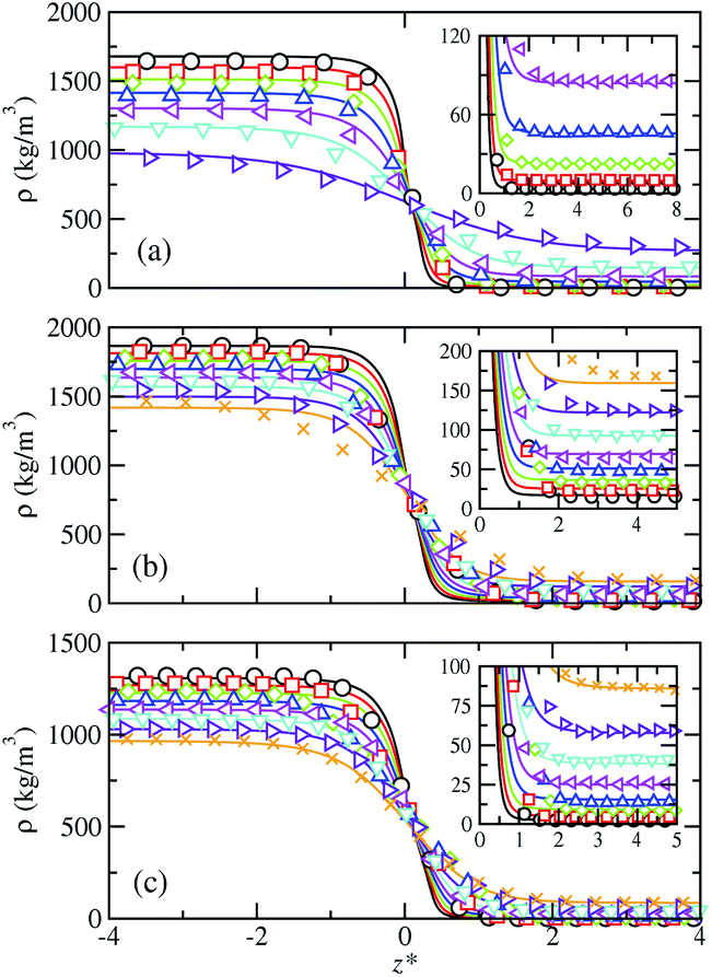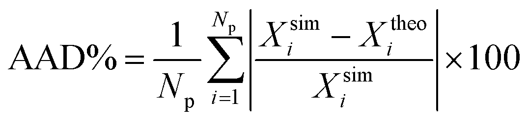
Fig. 1 Simulated and predicted equilibrium density profiles across the vapor–liquid interface as obtained from MD NVT simulations (symbols) and SAFT-VR Mie MF DFT (curves) using the CG Mie models for (a) SF₆, (b) CF₄, and (c) HFO-1234yf at the different temperatures. The colors for each fluid denote different coexistence temperatures. The different colors correspond to the temperatures collected in Table 1. The black color denotes each lowest considered temperature. The insets show an enlargement of the interfacial region next to the bulk vapor phase.

It is important to mention here that there exist other formalisms that are able to provide similar agreement with experimental data and computer simulation results taken from the literature.^40–42 However, the simple and direct approach presented here has several advantages over more sophisticated versions of DFT, such as those of Chapman and coworkers,⁶ and other formalisms, including the combination of the Helmholtz free energy of the SAFT-VR Mie equation of state with the Square Gradient Theory (SGT). From the perspective of functional theories, the combination of CG models, already developed in the literature, and the simple version of the DFT approach proposed in this work allows to use directly the same molecular parameters in a local functional algorithm easy to program and to solve. This is a clear advantage in comparison with other functionals that provide more detailed information but with a great computational effort. From the perspective of the SGT, the approach is not a strictly predictive tool, i.e., it needs some additional thermodynamic information, as well as the molecular parameters provided by the SAFT-VR Mie equation of state, to obtain reliable values of the influence parameter. Another drawback of SGT is that it can not be easily extended to deal with fluids in contact with solid surfaces and no simple solution can be obtained. This is not the case of DFT-based formalisms, for which the extension to non-local functionals can solve satisfactorily this issue. In summary, the simplified DFT version proposed and used in this work allows to get accurate predictions of the vapour–liquid interfacial tension of complex molecules with relatively low computational efforts.

2 Methodology

In this section we summarize the used molecular models and expose the simulation details. A comprehensive description of the theory can be found in our previous work.³⁷

2.1 Molecular models

Jackson and coworkers have proposed a number of force fields for different substances named generally SAFT-γ CG force fields.^27–30,43 They are based on a coarse-graining approach that models real substances as Mie molecular chains. We use this information provided by the group of Jackson and collaborators and use the CG models developed by them to predict the vapor–liquid interfacial properties of real complex substances using the DFT approach proposed by Algaba et al.³⁷ In particular, we concentrate here on two greenhouse gases, CF₄ and SF₆, as well in the HFO-1234yf refrigerant molecule. They are represented as a single-segment and a two-segment CG models, respectively. We also consider heavier molecules, n-decane (n-C₁₀H₂₂) and n-eicosane (n-C₂₀H₄₂). However, this becomes however increasingly inappropriate as the molecules become more elongated; the marked non-sphericity has to be accounted for explicitly. Hence, the n-C₁₀H₂₂ or C₁₀ and n-C₂₀H₄₂ or C₂₀ n-alkanes are modelled as fully-flexible homonuclear chains comprised by several tangentially bonded CG Mie segments, each corresponding to the CG functional groups required to adequately represent the chemical moieties. We use in this work the optimized CG parameters for the segment–segment interactions from the original paper of Avendaño et al.²⁸

However, when the number of chemical groups forming the molecules increases, which in the present case corresponds to an increase of the chain length, the Wertheim's first-order thermodynamic perturbation theory, or more precisely, the linear approximation for the many-body distribution function of the monomer reference fluid is not good enough to provide an accurate description of all thermodynamic properties of these compounds, including phase equilibria. This is one of the well-known limitations of Wertheim's theory at the level of the first-order perturbation.⁴⁴ According to the original version of the theory and later versions of the formalism, higher-order terms of the theory require the knowledge of many-body correlation functions, which are usually unknown as functions of temperature and density of the system for a given intermolecular potential. The simplest, and until now the only, solution is to assume that the higher-order many-body functions are uncorrelated up to the two-body level. Under this hypothesis, higher-order distribution functions can be expressed in terms of pair (two-body) distribution functions. This produces a less accurate description of the vapour and liquid densities, vapour pressures, and interfacial tensions, among other properties, of chain molecules as the chain length is increased. Further details on these issues can be found in the seminal works of Wertheim,⁴⁴ of Chapman and coworkers,¹⁸ and in the excellent review of Emborsky et al.⁶

One of the simplest solutions for improving the predictions of the theoretical approach is to scale the size and energy parameters using a single-stage scaling procedure with a limited set of simulated data, as explained in detail by Avendaño and coworkers.²⁸ In this work, in addition to the optimized size and energy parameters for all the substances considered, we also use the scaled parameters for C₁₀ and C₂₀ collected from the their work.

2.2 Simulation details

In addition to theoretical calculations, we perform computer simulations of the same models in order to establish a comparison of the obtained equilibrium and interfacial properties. In this work, we use the approach proposed by Müller et al.⁴⁵ to define the number of molecules and the size of the simulation box. Particularly, we use the phase equilibria predictions obtained from the SAFT-VR Mie EoS. According to this, the number of molecules and the size of the simulation box used for each compound are presented in Table 1. We also provide the value of the segment size used for each compound, as obtained by Avendaño and coworkers,²⁸ that allows to obtain all the relevant lengths in reduced units. We use a cutoff distance equal to 7σ. As can be seen, we use in all cases L_x = L_y = 14σ, being σ the monomeric diameter used in this work for each substance. This ensures the use of a cut-off radius r_c ≤ 7σ, half of the simulation length along the x- and y-axis. With these values, we do not expect dependence of surface tension with L_x and L_y.^46–48

Table 1 Values of the cut-off radius, r_c, segment size, σ, number of molecules, N, length of the simulation box along the x- and y-axis, L_x, L_y, and length of the simulation box along the z-axis, L_z, used in the MD NVT simulations for the substances considered

Substance	rc (nm)	σ (nm)	N	Lx, Ly (nm)	Lz (nm)
CF4	3.045	0.4350	5400	6.090	39.894
SF6	3.4027	0.4861	5400	6.8055	53.10
HFO-1234y	2.73	0.39	2700	5.460	39.60
C10	3.222	0.4603	1800	6.445	41.427
C20	3.1094	0.4442	900	6.445	41.427

---

It is important to take into account that in fully-flexible chain molecules, the end-to-end dimension of the chains is of the order of ∼m^1/2. For the case of the longest molecules considered in this work, C₂₀, that are modelled as a tangent chain formed by m_s = 6 CG monomeric segments, the end-to-end distance is approximately 2.45σ. This value is much lower than the dimensions of the simulation length along the x- and y-axis, which ensures that molecular chains are not correlated with their periodic images along these two axis. Also note that studies with longer chain-like molecules, formed by up to 16 monomeric units, have been previously simulated with similar sizes of simulation boxes.^49,50

Since liquid density, ρ_L, and vapor density, ρ_V, vary along the coexistence curve of each substance, the number of molecules and L_z for each fluid are chosen appropriately to ensure that the systems exhibit the correct phase behaviour, including two non-interacting vapor–liquid interfaces separated appropriately. In other words, the three slabs (vapour, liquid, and vapour phases) are thick enough to ensure that the equilibrium properties of each phase can be calculated correctly.

Particularly, we have checked that the width of the liquid slab between the two interfaces formed in the simulation box is large enough to ensure that correlations between the particles located at both interfaces are negligible. The number of molecules and the size of the simulation box along all the axis, including the z direction, is kept constant during the simulations (L_z > 90σ, according to Table 1). However, as the temperature of the system is higher, the distance between the two VL interfaces becomes shorter. The reason is directly related with the increasing of the VL interfacial thickness as T → T_c, which eventually diverges at T = T_c. The width of the liquid slab between the two VL interfaces of CF₄, SF₆, HFO-1234yf, C₁₀ and C₂₀ is always between 5 and 7.8 nm (CF₄), 6.4 and 9.3 nm (SF₆), 7.1 and 8.5 nm (HFO-1234yf), 8.9 and 9.3 nm (C₁₀) and 6.5 and 7.5 nm (C₂₀). The lower values correspond to the widths of the liquid slabs for the highest temperature considered and the higher values to those for the lowest temperature studied. These width values are higher than 14σ in all cases, being σ the segment size of each substance according to Table 1. The only exception is CF₄, for which the width is always larger than 12σ (σ = 0.435 nm).

We use the GROMACS (version 4.6.1)³⁹ simulation package to perform MD NVT simulations. We use the Verlet leapfrog⁵¹ algorithm with different time steps depending on the system. For CF₄ and SF₆, we use 2 fs, whereas for the rest of systems we use 1 fs. A Nosé-Hoover thermostat⁵² with large time constant equal to 2.0 ps has been used. Simulations of the vapor–liquid interfaces of CF₄ and SF₆ are equilibrated during 30 ns and HFO-1234y, C₁₀, and C₂ during 20 ns. The equilibrium properties are then obtained from averages over 70 ns in the case of CF₄ and SF₆ and during 30 ns in the rest of the systems. Uncertainties are estimated using the sub-block average method,⁵³ dividing the average period into M blocks. The statistical error for normal and tangential components of the macroscopic pressure tensor, vapor pressure, and surface tension are then estimated as , with [small sigma, Greek, macron] the variance of the block averages and M = 10.

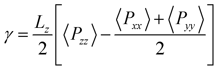
Thee equilibrium vapour pressure, P, and the surface tension, γ, are determined using the pressure tensor. P is equal to the normal component of the tensor and γ is evaluated as,^54–57

The factor 1/2 appears because we simulate two vapour–liquid interfaces. L_z is the length of the simulation box along the z-axis. Here z is perpendicular to the vapour–liquid planar interfaces.

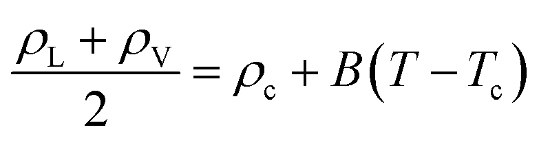
We have also determined the critical pressure (P_c), temperature (T_c), and density (ρ_c) according to the scaling and rectilinear diameters laws,^58,59

ρ_L − ρ_V = A(T − T_c)^β (2)

andβ = 0.325 is the Ising critical exponent.⁵⁵ A, B, T_c and ρ_c are determined by fitting eqn (2) and (3) to simulation data. ρ_L and ρ_V are the liquid and vapour coexistence densities at a given T.

It is also possible to calculate an alternative but complementary value of the critical temperature using the scaling law for the surface tension,⁵⁵

γ = γ₀(1 − T/T_c)^μ (4)

where γ₀ represents the “zero-temperature” interfacial tension and μ is the critical exponent associated to γ, which is set equal to the universal Ising value (μ = 1.258).⁵⁵ γ₀ and T_c are evaluated by fitting eqn (4) to simulation results.

Finally, P_c is determined evaluating P at T = T_c, obtained from eqn (2), using the Clausius–Clapeyron equation,

C₁ and C₂ are adjustable parameters obtained from the fitting of eqn (5) to the simulated pressure values.

3 Results

In this work, we use the DFT formalism to investigate the interfacial properties and the phase equilibria of five different molecular systems, namely CF₄, SF₆, HFO-1234y, C₁₀, and C₂₀ at coexistence conditions. The behavior obtained using the SAFT-VR Mie MF DFT approach is compared with computer simulation predictions using the same the models. The reliability of these results is supported by experimental data from the literature.

When a DFT approach is proposed to predict the interfacial behavior of a given system, the first magnitude to be considered and analyzed is the density profile. It provides structural information of the system and a first insight of the ability of the theoretical framework to predict the correct behavior of density along the interface. Note that an accurate description of density profiles is key to ensure a reliable description of other interfacial properties, including the interfacial tension.

Since we are dealing with planar interfaces, the density is a function of z, i.e., ρ = ρ(z), with z the position along the z-axis. Note that this direction has been chosen arbitrary as perpendicular to the interface. According to this, we first explore the density profiles of the five compounds considered in this work. Fig. 1 and 2 show the vapor–liquid density profiles, as functions of the distance from the interface, at different temperatures in the vapor–liquid coexistence region for each target fluid. The particular temperatures considered for each fluid are listed in Table 2. Density profiles for fluids modeled by a single (SF₆ and CF₄) and two (HFO-1234yf) CG Mie segments are shown in Fig. 1, and those for the large hydrocarbons modeled as chains are depicted in Fig. 2. We only plot one half of the density profiles corresponding to one of the interfaces and shift them along z-axis in order to place the Gibbs-dividing surface at the origin. Note that the insets of all figures show the interfacial region near the vapor bulk phase of the systems.

Fig. 2 Simulated and predicted equilibrium density profiles across the vapor–liquid interface as obtained from MD NVT simulations (symbols) and SAFT-VR Mie MF DFT (curves) using the CG Mie models for (a) C₁₀ and (b) C₂₀ at different temperatures. The colors for each fluid denote different coexistence temperatures.The different colors correspond to the temperatures collected in Table 2. The black color denotes each lowest considered temperature. The insets show an enlargement of the interfacial region next to the bulk vapor phase.

Table 2 Liquid (ρ_L) and vapour (ρ_V) densities, vapour pressure (P) and interfacial tension (γ), as functions of T, determined from computer simulations (NVT) for CF₄, SF₆, HFO-1234y, C₁₀, and C₂₀. Results for C₁₀ and C₂₀ are obtained using the optimized parameters of Avendaño and collaborators.²⁸ Results obtained using the scaled parameters are not presented here since can be obtained easily using the corresponding scaling factors. The errors are estimated as explained in the text

T (K)	ρL (kg m^−3)	ρV (kg m^−3)	P (MPa)	γ (mN m^−1)
CF4
135	1644(1)	3.67(8)	0.0454(8)	15.9(8)
150	1568.7(9)	10.2(1)	0.136(2)	13.07(8)
165	1486(1)	22.8(2)	0.325(2)	9.96(8)
180	1394(1)	45.7(3)	0.67(2)	7.33(6)
195	1289.1(9)	85.2(4)	1.246(7)	4.73(7)
210	1161.7(9)	149.9(5)	2.09(1)	2.43(6)
225	958(2)	288(2)	3.286(5)	0.74(5)
SF6
220	1866(1)	15.2(2)	0.183(2)	11.28(9)
230	1824(1)	23.3(2)	0.281(2)	10.2(1)
240	1779(1)	33.1(3)	0.412(2)	8.7(1)
250	1730(1)	47.4(3)	0.593(3)	7.3(1)
260	1674(2)	65(1)	0.801(4)	5.9(2)
270	1614(1)	92(1)	1.101(3)	4.8(1)
280	1547(1)	126(1)	1.463(8)	3.57(8)
290	1469(2)	169(2)	1.896(7)	2.40(6)
HFO-1234y
225	1318(1)	2.4(1)	0.039(2)	17.9(2)
240	1277(1)	4.8(2)	0.083(2)	15.8(2)
255	1232(2)	9.4(2)	0.162(3)	13.9(2)
270	1189(2)	13.3(5)	0.269(4)	11.5(2)
285	1139(3)	24.7(8)	0.506(9)	9.5(2)
300	1090(3)	39.9(8)	0.787(6)	7.4(2)
315	1036(3)	55.9(7)	1.13(1)	5.8(1)
330	982(3)	79.4(4)	1.641(9)	4.0(1)
C10
300	724(5)	0.016(2)	0.0008(5)	25.3(3)
330	699(5)	0.082(5)	0.0018(8)	22.8(2)
360	674(4)	0.34(2)	0.0069(8)	19.3(2)
390	647(5)	2(2)	0.023(1)	16.8(2)
420	620(6)	2.72(8)	0.064(3)	14.0(2)
450	592(5)	5.5(2)	0.134(2)	10.9(1)
480	561(5)	10.9(2)	0.266(4)	8.6(2)
510	527(7)	19.3(2)	0.488(8)	6.33(8)
540	486(1)	32.0(4)	0.786(9)	4.2(1)
C20
350	770.8(7)	—	0.0034(5)	25.0(3)
400	732.3(5)	0.006(2)	0.0029(5)	20.8(2)
450	692.7(5)	0.130(5)	0.0044(9)	17.1(2)
500	652.7(7)	0.96(9)	0.014(2)	13.4(2)
550	609.5(4)	2.9(1)	0.049(2)	10.1(2)
600	560.5(8)	9.4(4)	0.146(3)	7.3(2)
650	506.5(5)	22.8(2)	0.358(8)	4.2(1)
700	431(2)	55.3(7)	0.710(9)	2.1(2)

---

The obtained density profiles exhibit the expected shape as well as qualitative behavior with increasing temperature: liquid density decreases, vapor density increases, and the absolute value of the slope of the density profiles in the interfacial region decreases. In terms of the structure of the interface, density profiles show sharp interfaces at low temperatures, related with high values of the surface tension, and profiles broader as the temperature increases approaching to the critical point. Overall, we have found good agreement between theoretical predictions and MD NVT computational results for the bulk liquid and vapor densities. However, some quantitative differences are non-negligible and increase as the temperature is raised. The theory overestimates the density of the vapor-like region and underestimates the density in the liquid-like region. This is especially noticeable for the large alkanes and can be ascribed to the approximations made in the construction of the density functional: in the mean-field version of the theory, correlations between pair molecules due to the attractive interactions are neglected. This likewise would explain the major disagreement at high temperatures since using correct density fluctuations is crucial when the systems approach the critical temperature. The theory is thus unable to quantify the variation of the density along the interface for certain systems and thermodynamic conditions. In regards the interfacial region, SAFT-VR Mie MF DFT predicts it quite accurately in the case of the long alkanes, whereas narrower interfaces compared to simulation data can be observed at the lowest temperatures for the smaller molecules modelled as single and two CG segments.

The theoretical predictions obtained from the DFT approach considered in this work do not provide, as well as other theoretical approaches, including the traditional combination of the SAFT-VR Mie equation of state with SGT,^45,63 structural information of the possible preferential orientation and changes of conformation of chain molecules along the interfacial region. However, computer simulation allows one to visualize microscopic effects of the system at the interface. Our simulations indicate that none of the systems considered in this work exhibit preferential orientation nor changes in conformation across the interface. A priori, the only targeted molecules susceptible to suffer these effects are C₁₀ and C₂₀, which are comprised by m_s = 3 and 6 monomeric units, respectively. According to our previous results, fully flexible chains formed by up to six monomeric units interacting through the Mie intermolecular potential do not show these effects at interfaces. This is also corroborated by previous studies of Blas and MacDowell^49,50 involving fully flexible Lennard-Jones (LJ) chains. According to these authors, LJ chains formed by 4, 8, 12, and 16 segments do not exhibit preferential orientation neither other intramolecular effects along planar interfaces. The absence of these behaviours are also corroborated looking at the interface with the eyes of MD. Fig. 3 shows the snapshot extracted from MD trajectories of the simulation of C₂₀ (modelled as a Mie chain formed by m_s = 6 segments). As it can be observed, there is no preferential orientation of the molecules at the interface. In addition, there is no change in conformations of the molecules across the interface, as it is expected due to the molecular flexibility of the model.

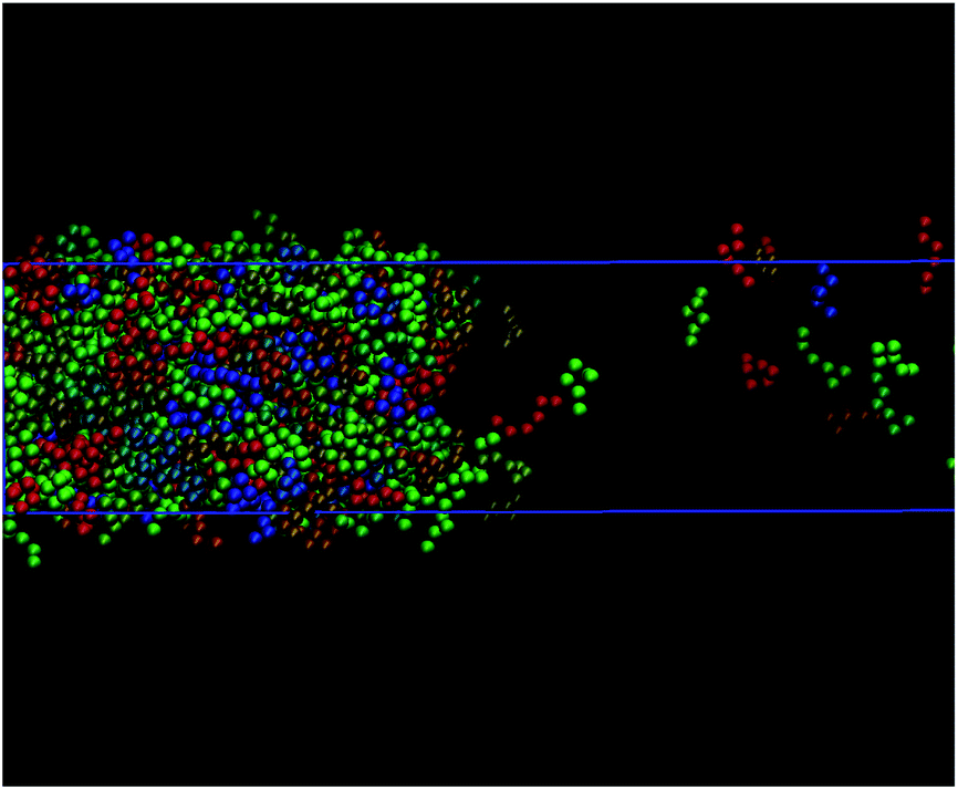Fig. 3 Snapshot of the VL interface obtained from MD NVT simulations of C₂₀ at 650 K. CG segments of each molecule are represented by spheres with the same color (van der Waals representation). Random different colors are used for different molecules.

Using SAFT-VR Mie MF DFT theory, we have also determined the vapor–liquid coexistence diagram for the target fluids and compared the predictions with those from molecular simulation, which are obtained from the information of the density profiles ρ(z) at coexistence temperatures. A summary of the results obtained from MD simulations is presented in Table 2. In addition to that, Table 3 includes the percentage average absolute deviation AAD% of the theory with respect to the simulation data:

where X^sim_i and X^theo_i are the simulated and theoretical properties, respectively. This provides a measure of the accuracy of the theory with respect to simulation results. This is particularly useful in the case of interfacial thickness and surface tension since allows to assess the quality of the theoretical predictions for interfacial properties. Note that scaled parameters for C₁₀ and C₂₀ are only provided for vapour pressure and surface tension, properties specifically evaluated using these sets of parameters. Critical constants as obtained from computer simulations using the procedure described in Simulation details section using eqn (2)–(5) are presented in Table 4. The critical temperature of each substance can be determined using the vapour and liquid coexistence densities, at each temperature, and fitting them to eqn (3), as it is explained in Simulation details section. Particularly, β is set equal to the value of the Ising critical exponent, β = 0.325, and A and T_c are obtained from a standard linear regression analysis. These results correspond to the T^†_c values shown in Table 4. The critical density is obtained in a similar way, i.e., using the same data (vapour and liquid densities) but fitting to eqn (3). Now, we use the critical temperature obtained previously, and B and ρ_c are obtained from a standard linear regression. We have also included the experimental critical temperatures and pressures taken from the literature^60–62 for comparison. Particularly, the bulk vapor and liquid densities are obtained by averaging ρ(z) over appropriate regions sufficiently removed from the interfacial region. In the case of the bulk vapor density their values are obtained averaging on both sides of the liquid film. Statistical uncertainties are estimated using the standard deviation of the averages. The corresponding coexistence curves are presented in Fig. 4. Additionally, we have included experimental data taken from literature for HFO-1234yf,⁶⁰ C₁₀ and C₂₀,⁶¹ and from the NIST database for the rest of fluids.⁶² As can be seen, predictions from both methods provide the correct curvatures and quantitative agreement is excellent in a wide range of temperatures, though a small systematic overestimation at the highest temperatures of coexistence is apparent. It means, the saturated liquid and vapor densities are well predicted but slight deviations from experiments are evident near the critical point. This is especially notable for the largest considered molecule, namely C₂₀ n-alkane. Quantification of the agreement between theory and simulation for the coexistence densities is provided in Table 3. Nearly the same AAD% values obtained by Avendaño and collaborators are also obtained here.²⁸

Table 3 Percentage average absolute deviation AAD% of the theoretical predictions with respect to the simulation data for the liquid (ρ_L) and vapour (ρ_V) densities, vapour pressure (P), interfacial thickness (d) and interfacial tension (γ) of CF₄, SF₆, HFO-1234y, C₁₀, and C₂₀. Results for C₁₀ and C₂₀ and for the corresponding scaled calculations are obtained using the optimized and scaled parameters of Avendaño and collaborators, respectively.²⁸

Substance	AAD (ρL)	AAD (ρV)	AAD (P)	AAD (d)	AAD (γ)
CF4	2	13	2	22	15
SF6	2	7	8	29	4
HFO-1234y	0.6	4	5	16	8
C10	0.18	27	27	15	12.1
C10 (scaled)	3	9	9	—	2
C20	0.4	57	69	21	23
C20 (scaled)	9	25	36	—	9

---

Table 4 Experimental (T^exp_c, ρ^exp_c, and P^exp_c) and predicted (T^†_c, T^§_c, ρ^†_c, and P^†_c) critical temperatures, densities, and pressures of CF₄, SF₆, HFO-1234y, C₁₀, and C₂₀. Critical temperatures, T^†_c and T^§_c, are determined using eqn (2)–(4), ρ^†_c using eqn (3), and P^†_c combining eqn (5) and the T^†_c value determined using eqn (2). Experimental data for substances are taken from the literature.^60–62

Substance	T^expc (K)	T^†c (K)	T^§c (K)	ρ^expc (kg m^−3)	ρ^†c (kg m^−3)	P^expc (MPa)	P^†c(MPa)
CF4	227.51	231(5)	233(2)	625.66	606(7)	3.75	3.91(8)
SF6	318.733	327(1)	319(4)	743.81	750(10)	3.75455	4.4(2)
HFO-1234y	367.85	377(2)	376(6)	478	740(20)	3.382	4.4(3)
C10	617	616(2)	613(5)	233	228(4)	2.11	2.4(3)
C20	768	745(2)	750(9)	241.578	227(4)	1.1746	1.10(10)
C10 (scaled)	617	627(2)	624(5)	233	224(4)	2.11	2.4(3)
C20 (scaled)	768	789(2)	795(9)	241.578	218(4)	1.1746	1.12(10)

---

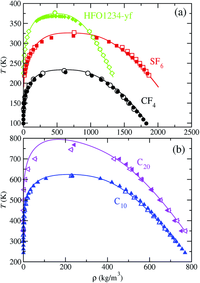Fig. 4 Vapour–liquid coexistence densities of (a) CF₄, SF₆, and HFO1234-yf, and (b) C₁₀ and C₂₀. The open symbols correspond to the coexistence densities obtained from MD NVT simulations, filled symbols to the experimental data taken from the literature,^60–62 and continuous curves to the SAFT-VR Mie MF DFT predictions using the CG Mie models for CF₄ (black circles and continuous curves), SF₆ (red squares and continuous curves), HFO-1234yf (green diamonds and continuous curve), C₁₀ (blue up triangles and continuous curve), and C₂₀ (blue up triangles and continuous curve). Symbols at the highest temperatures for each coexistence curve represent the critical points estimated from eqn (2) and (3) and the experimental critical points taken from the literature.^60–62

As we have mentioned previously in the Introduction, one of the main goals of this work is to assess if the theoretical approach describes accurately the interfacial properties of the CG models already presented. We have checked that the local SAFT-VR Mie DFT formalism, at the mean-field level of approximation, is able to predict reasonably well one of the key structural properties not directly accessible from experiments: the density profiles. Now, we concentrate on another structural property that also allows to quantify the accuracy of the theoretical framework in predicting this kind of properties.

Fig. 5 shows the 10–90 interfacial thickness, as a function of temperature, for the molecular models considered. We define the width of the interface, d, in the usual way, i.e., the distance over which the density changes from ρ_V + 0.1(ρ_L − ρ_V) to ρ_V + 0.9(ρ_L − ρ_V), with ρ_L and ρ_V the liquid and vapour coexistence densities evaluated in the bulk regions of the corresponding density profiles as obtained from simulation and theory. Table 5 also includes the values of d from both approaches at each temperature considered in Table 2.

Fig. 5 Interfacial thickness, as a function of temperature, of (a) CF₄, SF₆, and HFO1234-yf, and (b) C₁₀ and C₂₀. The open symbols correspond to the interfacial thickness obtained from MD NVT simulations and continuous curves to the SAFT-VR Mie MF DFT predictions using the CG Mie models for CF₄ (black circles and continuous curves), SF₆ (red squares and continuous curves), HFO-1234yf (green diamonds and continuous curve), C₁₀ (blue up triangles and continuous curve), and C₂₀ (magenta left triangles and continuous curve).

Table 5 Simulated (d^†) and predicted (d^§) interfacial thickness for CF₄, SF₆, HFO-1234y, C₁₀, and C₂₀ as obtained from the analysis of the density profiles calculated from MD NVT simulations and the SAFT-VR Mie MD DFT formalism, respectively

T (K)	d^† (nm)	d^§ (nm)
CF4
120	0.456(13)	0.447
135	0.703(24)	0.573
150	1.00(3)	0.715
165	1.38(3)	0.863
180	1.40(3)	1.097
195	1.855(20)	1.563
210	2.60(5)	2.001
225	5.09(6)	3.610
HFO-1234y
225	0.916(5)	0.780
240	1.025(5)	0.847
255	1.263(7)	0.936
270	1.481(15)	1.063
285	1.36(3)	1.209
300	1.56(4)	1.384
315	1.88(5)	1.638
330	2.15(7)	2.008
—	—	—
C20
350	0.751(5)	0.710
400	0.894(6)	0.796
450	1.072(5)	0.941
500	1.408(6)	1.077
550	1.611(6)	1.266
600	1.901(7)	1.565
650	3.49(9)	1.977
700	4.07(4)	2.687
SF6
220	0.979(3)	0.690
230	1.154(3)	0.778
240	1.091(3)	0.861
250	1.535(5)	0.958
260	1.424(14)	1.060
270	1.85(9)	1.210
280	1.87(4)	1.385
290	2.14(4)	1.604
C10
300	0.715(10)	0.694
330	0.839(10)	0.768
360	0.917(5)	0.862
390	1.139(5)	0.957
420	1.289(5)	1.099
450	1.408(21)	1.253
480	2.27(3)	1.460
510	2.14(3)	1.749
540	2.864(16)	2.163

---

It is interesting to discuss the general trend of the interfacial thickness curves, as functions of temperature and for the different substances considered, taken into account the results presented for the density profiles (Fig. 1 and 2) and the coexistence curves (Fig. 4). According to the results shown in Fig. 5, d increases as the temperature of the systems is increased. This is the expected behaviour since the interfacial region becomes wider with temperature, in agreement with the trend followed by the coexistence densities as T increases (Fig. 4). Close to the critical region, the interfacial thickness increases more rapidly and eventually diverges as T → T_c. Note that all models exhibit the same qualitative behavior. The divergence of d with T is more evident in the case of CF₄ and less clear in the rest of the substances analyzed. This can be explained if we take into account the last value of d considered in Fig. 4 and Tables 2 and 5: in the case of CF₄, the last temperature considered is 225 K, that corresponds to 0.97T_c. In the rest of the systems, the last temperatures correspond to 0.91, 0.89, 0.87, and 0.91T_c for SF₆, HFO-1234yf, C₁₀, and C₂₀, respectively. This can be clearly seen in the corresponding coexistence curves shown in Fig. 4.

As can be seen in Fig. 5, the theory is able to capture the behaviour of the interfacial thickness obtained from computer simulation, especially at low temperatures, even in the case of the longest molecules studied, C₁₀ and C₂₀. Agreement between simulation and theory is good for the case of the shortest molecules (CF₄, SF₆ and HFO-1234y). Unfortunately, differences between both results is more important in the cases of SF₆ and C₂₀ (see also Table 3). In general, one can say that the theory is able to provide a reasonable agreement with computer simulation results if we take into account that results from the SAFT-VR Mie DFT formalism are pure predictions, without the use of any adjustable parameter. Fig. 5 demonstrates that the description of the interfacial region previously shown in Fig. 1 and 2 is remarkable, especially if we take into account that SAFT-VR Mie DFT is a formalism that treats short-range interactions in a local way and correlations due to the attractive interactions are neglected via a mean-field approximation of the perturbative term.

We have also determined the vapor pressure, as a function of temperature, for each fluid from theory and computer simulations, and comparison is shown in Fig. 6. Available experimental data is likewise included.^60–62 Critical pressures obtained from computer simulation are also presented in Table 4. The theoretical calculation of the vapor pressure involves the SAFT-VR Mie EoS, whereas for MD NVT simulations is obtained from the diagonal components of the pressure tensor, and particularly, from the normal component of the tensor. As it is clearly apparent from the figure, we found for this property the expected behavior: it decreases with increasing the molecular size and increases with increasing the temperature.

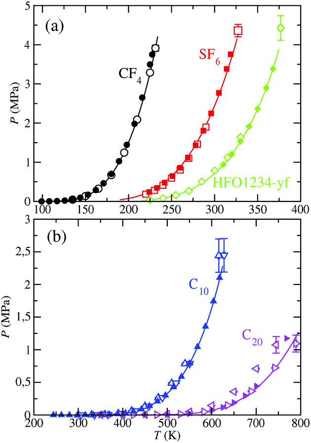Fig. 6 Vapour pressure of CF₄, SF₆, HFO-1234yf, C₁₀, and C₂₀. The meaning of the symbols is the same as in Fig. 5. Open blue down triangles and open magenta right triangles correspond to the vapor pressures obtained from MD NVT simulations using the scaled parameters for C₁₀ and C₂₀, respectively. Symbols at the highest temperature for each vapour pressure curve represent the experimental critical pressure taken from the literature and the critical pressure, corresponding to the simulations results, obtained from eqn (5) using the critical temperature values obtained from eqn (2).

The vapor pressure curves predicted from theory and computer simulation corresponding to the three compounds with the lowest molecular weight (part (a) of the figure) are in excellent agreement with experimental data taken from the literature, even near the critical region. However, the critical pressures obtained from SAFT-VR Mie EOS and simulation overestimate their experimental values (see Table 4 for further details). As we have mentioned previously, this is expected since the SAFT-VR Mie formalism, as other SAFT approaches and classical EOS, neglect the fluctuations of the system near the critical region. It is also expected that the predictions obtained from simulations would overestimate the experimental critical pressures since the CG models are based on that equation.

In regards to the vapor pressures of the C₁₀ and C₂₀ alkanes (part (b) of Fig. 6), SAFT-VR Mie predictions accurately match experimental data in the whole range of coexistence conditions. MD NVT computer simulations with optimized molecular parameters for the CG models describe appropriately the vapor pressures at low and intermediate temperatures for these long molecules but their vapor pressures at high temperatures are overestimated, especially in the case of C₂₀. It is worth noting however that using the scaled parameters for the CG models reported by Avendaño et al.,²⁸ molecular simulation is also able to provide an excellent quantitative agreement of the vapor pressures curves of C₁₀ and C₂₀ in the whole range of temperatures considered. See also Table 3 for further details.

For completeness, we compute the vapor–pressure curve in its Clausius–Clapeyron representation, which is depicted in Fig. 7. It allows one to better assess the results at low and intermediate temperatures. Although the accurate description of the vapor pressures of long-chain hydrocarbons at the low temperatures is commonly challenging, our calculations are able to successfully predict their values at these conditions. As well, the obtained slope of this vapor–pressure curve accurately agrees with the experimental data for all the considered fluids. The description of the vapor pressure using the SAFT-γ Mie force fields is overall highly efficacious taken into account the simplicity of these CG models. It is worth to remind here the importance of using scaled parameters for n-decane and more particularly for n-eicosane,²⁸ as we have mentioned in the previous section.

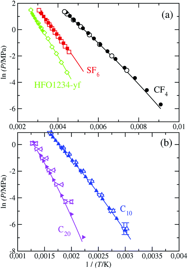Fig. 7 Clausius–Clapeyron representation of the vapour pressure of CF₄, SF₆, HFO-1234yf, C₁₀, and C₂₀. The meaning of the symbols is the same as in Fig. 6.

Finally, we have used the SAFT-VR Mie MF DFT formalism to determine the vapor–liquid surface tension of the models studied here. As for the vapor pressure, the interfacial tension is computationally obtained from the diagonal components of the pressure tensor. Particularly, it is determined from the difference of the averages of the normal and tangential components of the macroscopic pressure tensor. The interfacial tension, as a function of temperature, for each studied fluid is shown in Fig. 8. The interfacial tension values obtained from MD simulations are also presented in Table 2 and the corresponding percentage average absolute deviations AAD% are listed in Table 3. We have also obtained the critical temperature of each substance using the interfacial tension values as functions of temperature. This can be done using the γ values at each T and fitting them to eqn (4). Particularly, μ is set to the Ising universal value, μ = 1.258, and γ₀ and T_c are treated as adjustable parameters obtained from a standard linear regression. The critical temperature T^§_c values are presented in Table 4. Differences between T^†_c (obtained from the analysis of ρ_V and ρ_L as functions of temperature) and T^§_c (obtained from the analysis of γ as function of T) are usually seen in computer simulation studies.^{49,50,64–68} In this particular case, differences between T^†_c and T^§_c are below 1% in all cases except for the SF₆ system, in which discrepancies are ∼2%. This is probably due to finite-size effects of the simulation box used that affect in a different way to the coexistence densities and interfacial tensions, producing slightly differences between the critical temperatures obtained from these two alternative but complementary routes. We have also included the experimental data taken from the literature to assess the ability of the theoretical approach in describing this key interfacial property. As it can be seen, theoretical and computer simulation predictions are able to provide an accurate description of the surface tension of all the fluids. In particular, they predict the correct and expected shape characteristic of non-associating systems.

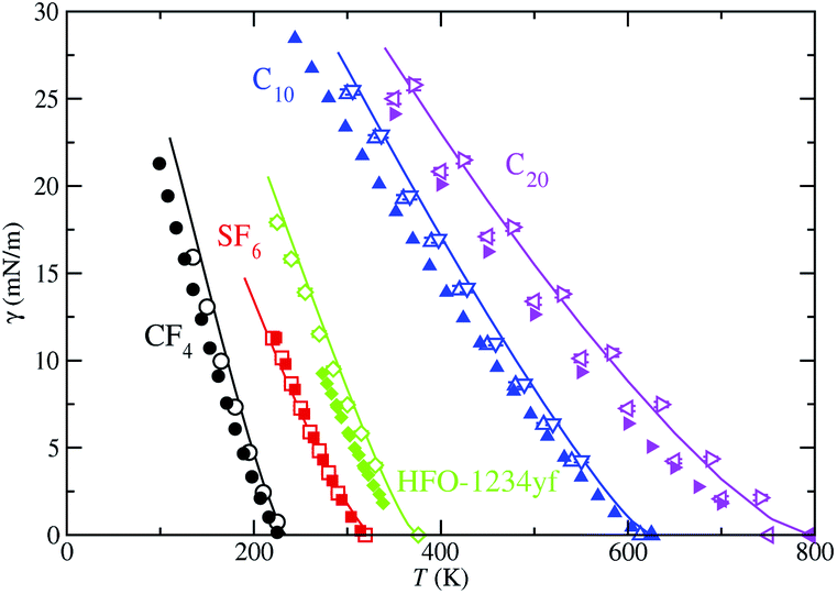Fig. 8 Vapor-liquid surface tension as a function of temperature for CF₄, SF₆, HFO-1234yf, C₁₀, and C₂₀. The meaning of the symbols is the same as in Fig. 5.

As in the case of vapor pressure, we first discuss the results obtained for the vapor–liquid interfacial tension of the lighter compounds considered (CF₄, SF₆, and HFO-1234yf). As can be seen, the SAFT-VR Mie MF DFT is able to provide an excellent description of the vapor–liquid interfacial tension of SF₆ in the whole range of temperatures. Computer simulation results for the corresponding CG model are also in very good agreement with theory and experiments. However, although the theoretical and computer simulation predictions of the surface tension of CF₄ and HFO-1234yf are good at all temperatures, some discrepancies are observed. Simulation results slightly overestimate the experimental data of these substances, especially at low temperatures. In addition to that, SAFT-VR Mie MF DFT formalism overestimates the surface tension values at low temperatures. This an expected behavior since it neglects correlations of the attractive interactions of the systems, leading lower cohesive energies and consequently, higher values of the vapor–liquid surface tension. A more sophisticated version of the functional proposed here, that would include correlations for the long-range attractive interactions, would provide better predictions for the surface tension.

A more detailed description of the results obtained deserves the comparison among theory, computer simulation, and experiments for n-alkanes. As in the case of vapor pressures, here we also use the optimized and the scaled molecular parameters of Avendaño and collaborators.²⁸ SAFT-VR Mie MD DFT is able to provide a reasonably good description of the vapor–liquid interfacial tension. Agreement between theoretical predictions and experimental data taken from the literature is better at high temperatures, increasing the discrepancy with decreasing the temperature. However, in general, theory overestimates experimental values for interfacial tension of n-alkanes. This behavior is expected, as we have mentioned previously since the theory neglects correlations between molecules at the long-range attractive interactions level. These differences are larger in the case of C₂₀ than those in C₁₀ due to the nature of the intrinsic approximations of Wertheim's first-order thermodynamic perturbation theory associated to the chain formation contribution.

Computer simulations of the CG models reported by Avendaño and coworkers,²⁸ using the optimized parameters, provide an excellent description of the vapor–liquid surface tension of n-alkanes. Particularly, good quantitative agreement with experimental data from the literature is observed at all temperatures, although some discrepancies are evident at low temperatures, especially in the case of C₁₀. Our computer simulation results are similar than those obtained by Avendaño and collaborators. It is observed however a slightly better agreement between both results in the current study probably due to different values used for the cut-off radius: they used a value r_c = 6σ whereas we use a larger value, r_c = 7σ. Here σ is the value of the segment size of n-alkanes given in Table 1. It is well known that surface tension is very sensitive in general to the molecular details, and in particular to the range of the attractive interactions.⁶⁹

Finally, we use the values of the scaled molecular parameters of n-alkanes proposed by Avendaño and coworkers to account for the interfacial tension of C₁₀ and C₂₀. It is important to recall here how the optimized and scaled parameters are obtained. The optimized parameters are generally obtained by fitting the SAFT-VR Mie EOS predictions to the experimental saturated liquid densities and vapor pressures at several temperatures along the vapor–liquid coexistence curve. The scaled parameters are determined from a refinement procedure of the optimized parameters that allows the CG models to describe accurately the SAFT-VR Mie predictions. As can be seen, the predictions obtained from simulations of the CG models using the scaled parameters are very similar than those obtained from the optimized parameters for the case of C₁₀. In the case of C₂₀, computer simulations clearly overestimate the experimental values taken from the literature and the predictions obtained from simulations using the optimized parameters. However, a careful inspection of Fig. 8 reveals an interesting behavior for the predictions obtained from the scaled parameters. Although simulations results for C₁₀ and C₂₀ using the scaled parameters overestimate systematically the experimental values, they are in excellent agreement with theoretical predictions obtained from the SAFT-VR Mie MF DFT approach. See also the AAD% values presented in Table 3 for a quantification of the differences between theory and simulation using the two sets of parameters. This result is expected since scaled parameters have been refined trying to account for the best description of the predictions of SAFT-VR Mie, and particularly, trying to account for eqn (4) and (5) of the paper of Avendaño et al.²⁸ From this perspective, CG models with scaled parameters and SAFT-VR Mie MF DFT treatments are fully consistent. This also indicates that an improvement of the free energy functional of the DFT approach, and particularly, a more accurate approximation for dealing with correlations of molecules at the long-range attractive interactions level, would significantly improve theoretical predictions from SAFT-VR Mie DFT.

4 Conclusions

In this work we apply the recently proposed density functional theory, the SAFT-VR Mie MF DFT approach,³⁷ to predict the vapor–liquid interfacial properties of representative and diverse chemical compounds with industrial and fundamental interest modeled using the SAFT-γ Mie force fields.²⁸ The results obtained are compared with those obtained by conducting MD NVT molecular simulations using the direct coexistence technique as well as with experimental data taken from the literature. Overall, SAFT-VR Mie MF DFT is able to predict accurately the bulk values of the vapor and liquid densities. Although the phase equilibria curves are accurately predicted, differences between the density predictions achieved by the theory and by MD simulations are evident when the target fluids approach the critical point. Experimental data for the vapor pressure, as a function of temperature, shows that the theory provides more precise quantitative results. This is especially apparent from the Clausius–Clapeyron representation, which allows one to better examine the results at low and intermediate temperatures. Although reproducing the relatively low values of vapor pressure of long alkanes at low temperatures is difficult, they are found in remarkable agreement with experiments. The theory is also able to predict correctly the surface tension values. However, both theoretical and computational predictions overestimate experimental data.

Overall, results of this work dealing with a variety of compounds point to the reliability of the simple SAFT-VR Mie MF DFT approach for the study of phase equilibrium and interfacial properties of pure fluids. The major deviations for the evaluated properties correspond to the large alkanes, being C₂₀ the most problematic, and to the highest temperatures of coexistence. Discrepancies between theory and simulation predictions for long-chain molecules is partly due to the linear approximation for the many-body distribution function of the monomer reference fluid, as we have previously mentioned and inherent to the Wertheim's first-order thermodynamic perturbation theory. However, differences in interfacial properties for long-chain n-alkanes can also partly arise from the approximations made in the construction of the density functional. In the mean-field version, correlations between pair molecules due to the attractive interactions are neglected. The importance of correct pair correlations becomes greater with both described situations: with increasing the molecular size, and when the systems approach the critical temperature. This can be a subject for future work.

To sum up, in this study the SAFT-VR Mie MF DFT theory³⁷ has been demonstrated a powerful tool for the prediction of interfacial properties of complex real molecules. The excellent agreement of the results with those obtained from molecular simulation and experimentally points to its reliability for characterizing inhomogeneous systems, with the advantage of its efficiency in time and computational efforts.

Conflicts of interest

The authors declare that they have no known competing financial interests or personal relationships that could have appeared to influence the work reported in this paper.

Acknowledgements

This work was financed by Spanish Ministerio de Economía, Industria y Competitividad (Grant No. FIS2017-89361-C3-1-P), Spanish Ministerio de Ciencia e Innovación (Grant No. PID2021-125081NB-I00), Junta de Andalucía (Grant No. P20-00363), both co-financed by EU FEDER funds, and Universidad de Huelva. We also acknowledge the Centro de Supercomputación de Galicia (CESGA, Santiago de Compostela, Spain) for providing access to computing facilities.

Notes and references

1. H. T. Davis, Statistical Mechanics of Phases, Interfaces, and Thin Films, VCH, Weinheim, 1996.
2. R. Evans, Density Functionals in the Theory of Nonuniform Fluids, in Fundamentals of Inhomogeneous Fluids, Dekker, New York, 1992.
3. H. Löwen, J. Phys.: Condens. Matter, 2002, 14, 11897–11905.
4. J. Wu, AIChE J., 2006, 52, 1169–1193.
5. J. Wu and Z. Li, Annu. Rev. Phys. Chem., 2007, 58, 85–112.
6. C. P. Emborsky, Z. Feng, K. R. Cox and W. G. Chapman, Fluid Phase Equilib., 2011, 306, 15–30.
7. D. Frenkel and B. Smit, Understanding Molecular Simulations, Academic, San Diego, 2nd edn, 2002.
8. M. P. Allen and D. J. Tildesley, Computer Simulation of Liquids, Oxford University PressClaredon, Oxford, 2 edn, 2017.
9. E. A. Müller and G. Jackson, Annu. Rev. Chem. Biomol. Eng., 2014, 5, 405–427.
10. W. G. Chapman, K. E. Gubbins, G. Jackson and M. Radosz, Fluid Phase Equilib., 1989, 52, 31–38.
11. W. G. Chapman, K. E. Gubbins, G. Jackson and M. Radosz, Ind. Eng. Chem. Res., 1990, 29, 1709–1721.
12. M. S. Wertheim, J. Stat. Phys., 1984, 35, 19–34.
13. M. S. Wertheim, J. Stat. Phys., 1984, 35, 35–47.
14. M. S. Wertheim, J. Stat. Phys., 1986, 42, 459–476.
15. M. S. Wertheim, J. Stat. Phys., 1986, 42, 477–492.
16. C. McCabe and A. Galindo, in Applied Thermodynamics of Fluids, ed. A. Goodwin, J. V. Sengers and C. J. Peters, Royal Society of Chemistry, London, 2010, ch. 8.
17. G. Jackson, W. G. Chapman and K. E. Gubbins, Mol. Phys., 1988, 65, 1–31.
18. W. G. Chapman, G. Jackson and K. E. Gubbins, Mol. Phys., 1988, 65, 1057–1079.
19. F. J. Blas and L. F. Vega, Mol. Phys., 1997, 92, 135.
20. F. J. Blas and L. F. Vega, Ind. Eng. Chem. Res., 1998, 37, 660.
21. J. Gross and G. Sadowski, Ind. Eng. Chem. Res., 2002, 41, 1084–1093.
22. A. Gil-Villegas, A. Galindo, P. J. Whitehead, S. J. Mills, G. Jackson and A. N. Burgess, J. Chem. Phys., 1997, 106, 4168–4186.
23. A. Galindo, L. A. Davies, A. Gil-Villegas and G. Jackson, Mol. Phys., 1998, 93, 241–252.
24. T. Lafitte, D. Bessieres, M. M. Piñeiro and J. L. Daridon, J. Chem. Phys., 2006, 124, 024509.
25. T. Lafitte, A. Apostolakou, C. Avendaño, A. Galindo, C. S. Adjiman, E. A. Müller and G. Jackson, J. Chem. Phys., 2013, 139, 154504.
26. C. Herdes, T. S. Totton and E. A. Müller, Fluid Phase Equilib., 2015, 406, 91–100.
27. C. Avendaño, T. Lafitte, A. Galindo, C. S. Adjiman, G. Jackson and E. A. Müller, J. Phys. Chem. B, 2011, 115, 11154–11169.
28. C. Avendaño, T. Lafitte, C. S. Adjiman, A. Galindo, E. A. Müller and G. Jackson, J. Phys. Chem. B, 2013, 117(9), 2717–2733.
29. O. Lobanova, T. Lafitte, C. Avendaño, E. A. Müller and G. Jackson, Mol. Phys., 2015, 113, 1228–1249.
30. G. J. O. Lobanova, A. Mejía and E. A. Müller, J. Chem. Thermodyn., 2016, 93, 320–336.
31. G. J. Gloor, G. Jackson, F. J. Blas, E. Martín Del Río and E. D. Miguel, J. Chem. Phys., 2004, 121, 12740–12759.
32. G. J. Gloor, G. Jackson, F. J. Blas, E. M. D. Río and E. D. Miguel, J. Phys. Chem. C, 2007, 111, 15513–15522.
33. F. J. Blas, E. Martín Del Río, E. de Miguel and G. Jackson, Mol. Phys., 2001, 99, 1851–1865.
34. G. J. Gloor, F. J. Blas, E. M. D. Río, E. D. Miguel and G. Jackson, Fluid Phase Equilib., 2002, 194–197, 521–530.
35. F. Llovell, A. Galindo, G. Jackson and F. J. Blas, J. Chem. Phys., 2010, 133, 024704.
36. F. Llovell, N. MacDowell, A. Galindo, G. Jackson and F. J. Blas, Fluid Phase Equilib., 2012, 336, 137–150.
37. J. Algaba, J. M. Míguez, B. Mendiboure and F. J. Blas, Phys. Chem. Chem. Phys., 2019, 21, 11937–11948.
38. J. M. Garrido, A. Mejía, M. M. Piñeiro, F. J. Blas and E. A. Müller, AIChE J., 2016, 62, 1781–1794.
39. D. van der Spoel, E. Lindahl, B. Hess, G. Groenhof, A. E. Mark and H. J. Berendsen, J. Comput. Chem., 2005, 26, 1701–1718.
40. A. Mejía, C. Herdes and E. A. Müller, Ind. Eng. Chem. Res., 2014, 53, 4131.
41. M. Chorążewski, M. Geppert-Rybczyńska, J. K. Lehmann, J. M. Garrido, A. Mejía and I. Polishuk, J. Chem. Thermodyn., 2019, 132, 222–228.
42. I. Polishuk, A. Chiko, E. Cea-Klapp and J. M. Garrido, Ind. Eng. Chem. Res., 2021, 60, 9624–9636.
43. T. Lafitte, C. Avendaño, V. Papaionnou, A. Galindo, C. S. Adjiman, G. Jackson and E. A. Müller, Mol. Phys., 2012, 110(11–12), 1189–1203.
44. M. S. Wertheim, J. Chem. Phys., 1987, 87, 7323–7331.
45. E. A. Müller, A. Ervik and A. Mejía, Living J. Comp. Mol. Sci., 2021, 2, 21385.
46. L.-J. Chen, J. Chem. Phys., 1995, 103, 10214.
47. M. González-Melchor, P. Orea, J. López-Lemus, F. Bresme and J. Alejandre, J. Chem. Phys., 2005, 122, 094503.
48. J. Janeček, J. Chem. Phys., 2009, 131, 124513.
49. F. J. Blas, L. G. MacDowell, E. D. Miguel and G. Jackson, J. Chem. Phys., 2008, 129, 144703.
50. L. G. MacDowell and F. J. Blas, J. Chem. Phys., 2009, 131, 074705.
51. M. A. Cuendet and W. F. V. Gunsteren, J. Chem. Phys., 2007, 127, 184102.
52. S. Nosé, Mol. Phys., 1984, 52, 255–268.
53. H. J. C. Berendsen, J. P. M. Postma, W. F. V. Gunsteren, A. D. Nola and J. R. Haak, J. Chem. Phys., 1984, 81, 3684.
54. H. Hulshof, Ann. Phys., 1901, 4, 165–186.
55. J. S. Rowlinson and B. Widom, Molecular Theory of Capillarity, Claredon Press, 1982.
56. E. D. Miguel, F. J. Blas and E. M. D. Río, Mol. Phys., 2006, 104, 2919–2927.
57. E. D. Miguel and G. Jackson, J. Chem. Phys., 2006, 125, 164109.
58. J. S. Rowlinson and F. L. Swinton, Liquids and Liquid Mixtures, Butterworth, London, 1982.
59. H. W. Xiang, The Corresponding-States Principle and Its Practice Thermodynamic, Transport and Surface Properties of Fluids, Elsevier, Amsterdam, 2005.
60. K. Tanaka and Y. Higashi, Int. J. Refrig., 2010, 33, 474–479.
61. DECHEMA Gesellschaft Für Chemische Technik Und Biotechnologie E.V., Frankfurt Am Main, Germany, https://cdsdt.dl.ac.uk/detherm/, retrieved July, 2011.
62. E. W. Lemmon, M. O. McLinden and D. G. Friend, in NIST Chemistry WebBook, NIST Standard Reference Database Number 69, ed. P. J. Linstrom and W. G. Mallard, National Institute of Standards and Technology, Gaithersburg MD, 2021.
63. A. Mejía, E. A. Müller and G. Chaparro Maldonado, J. Chem. Inf. Model., 2021, 61, 1244–1250.
64. E. Feria, J. Algaba, J. M. Míguez, A. Mejía, P. Gómez-Álvarez and F. J. Blas, Phys. Chem. Chem. Phys., 2020, 22, 4974–4983.
65. F. J. Martínez-Ruiz, F. J. Blas, B. Mendiboure and A. I. Moreno-Ventas Bravo, J. Chem. Phys., 2014, 141, 184701.
66. J. M. Garrido, M. M. Piñeiro, A. Mejía and F. J. Blas, Phys. Chem. Chem. Phys., 2016, 18, 1114–1124.
67. F. J. Blas, A. I. Moreno-Ventas Bravo, J. M. Míguez, M. M. Piñeiro and L. G. MacDowell, J. Chem. Phys., 2012, 137, 084706.
68. J. G. Sampayo, F. J. Blas, E. D. Miguel, E. A. Müller and G. Jackson, J. Chem. Eng. Data, 2010, 55, 4306.
69. A. Trokhymchuk and J. Alejandre, J. Chem. Phys., 1999, 111, 8510–8523.

---