The role of particulate matter in reduced visibility and anionic composition of winter fog: a case study for Amritsar city

Abstract

Severe fog events during winter months in India are a serious concern due to the higher incidence of road accidents, flight delays and increased occurrence of respiratory diseases. The present paper is an attempt to study the twenty fog samples collected from the rooftop of an academic building of Guru Nanak Dev University, Amritsar, India from November 2017 to January 2018. Fog samples were analysed for various parameters viz. pH, electrical conductivity (EC), chloride (Cl⁻), nitrate (NO₃⁻) and sulphate (SO₄²⁻) levels. The pH, EC, and Cl⁻, NO₃⁻ and SO₄²⁻ levels in the fog samples were estimated as 6.3–7.9, 240–790 μS cm⁻¹, 108–2025 μeq L⁻¹, 105–836 μeq L⁻¹ and 822–5642 μeq L⁻¹, respectively. It was noticed that sulphate was the dominant anion in fog samples. The SO₄²⁻ to NO₃⁻ molar ratio in the fog was estimated as 7.6 which suggests the burning of fossil fuel as the major pollutant from vehicular exhausts. Multiple regression analysis was performed to evaluate the effect of PM_2.5/PM₁₀ ratio and relative humidity (RH) on visibility. A box-cox plot of power transformation produced better model fitting, employing a square root transformation of the visibility which indicated that the PM_2.5/PM₁₀ and RH have an exponential effect on visibility.

---

1. Introduction

Global Risks Perception Survey ranked “climate action failure” as the world's top long-term hazard and the risk with the most severe possible consequences over the next decade.¹ The heavily populated Indo-Gangetic Plain (IGP) region is the hotspot of aerosol loading due to extremely elevated concentrations of fine particulate matter (PM_2.5), especially during the winter months.^2,3 The shallow planet boundary layer (PBL) and minimal wind during the winter months result in a decrease in ventilation coefficient that prevents the dispersion of pollutants to the upper atmosphere.^2,4 As per information by Road accidents in India (2017),⁵ fog and mist were responsible for 26 982 accidents. Fog episodes over northwest India occur primarily in the winter months (December–February). Ghude et al.⁶ have reported visibility as low as <50 m for 8 hours at Indira Gandhi International airport, New Delhi during the period of 7 and 8 January 2016. Due to a variety of names and divisions, fog is classified into different categories.⁷ According to the National Oceanic Atmospheric Administration (NOAA), fog is expressed as obscuration of horizontal visibility < 1 km caused by tiny water droplets in the atmosphere⁸ and relative humidity (RH) > 80%.⁹ Zhu et al.¹⁰ classified fog as dense fog (visibility in the range of 0.2–0.5 km) and heavy fog (visibility in the range of 0.5–1 km). During the fog formation stage, the PM_2.5 concentration decreases, but increases during the fog mature stage.

Thus, the ionic composition of fog is largely affected by local sources and/or transportation from long distances depending on meteorological conditions. The contribution from the long-distance range may be low due to the shrinking of PBL. Gao and Ji¹¹ reported maximum concentration of PM_2.5 (369 ± 112) μg m⁻³ exceeding 5 times National Ambient Air Quality Standards (NAAQS) of China during heavy fog and haze conditions of winter from September 2015 to August 2016 over Beijing. In the fog experiment over Delhi from December 2015 to February 2016, Ali et al.¹² reported that the calm atmosphere with minimum wind and low thickness of PBL (307 ± 325) m are causes of the high PM_2.5 (198.6 ± 55.6 μg m⁻³) in the winter months and sulphate (SO₄²⁻), chloride (Cl⁻) and nitrate (NO₃⁻) as dominant ions. Several researchers^13–17 have reported a higher concentration of particulate matter over Amritsar, a holy city of Punjab. Gu et al.¹⁸ investigated the long-term effects (1989–2017) of urbanisation on fog types in Shanghai and concluded that an increase in surface air temperature by 0.5–6.1 °C can reduce the incidence of fog formation. Along with air pollution, the interaction between various climatic parameters and their impact on visibility conditions in winter fog is something that needs to be addressed to avoid unintended causes in north India. There are limited studies on winter fog chemistry over Indian cities (Table S1†).

Forecasting visibility is very essential during foggy conditions in the winter season. A multiple linear regression (MLR) analysis has been performed between aerosol mass concentration and depression temperature on visibility in Delhi during winter months for two consecutive years. According to the regression analysis, visibility is better explained by two model terms (aerosol mass concentration and depression temperature) as compared to depression temperature as a sole independent variable.¹⁹ PM_2.5 showed a negative exponential function with visibility and PBL (R = 0.806) during fog-haze events over Beijing during 2014–2015.²⁰ Wang et al.²¹ studied the effect of PM_2.5 and RH on visibility in Beijing and suggested linear and exponential regression models as best fitted. This study reported both the PM_2.5 concentrations and RH contribute to atmospheric visibility. But, 50% variance in visibility was explained by PM_2.5 concentrations (<200 μg m⁻³) under low RH (<40%), whereas at high PM_2.5 load (>200 μg m⁻³) and high RH (>40%), the contribution of PM_2.5 is reduced to 10–15% in estimating the visibility. In another study carried out at Indira Gandhi International (IGI) airport, New Delhi reported that the visibility and RH had a negative correlation (R = −0.85, p < 0.0001) during December 2015–February 2016.²² Won et al.²³ have applied a censored regression model due to a narrow range of visibility and found that PM_2.5 has a more profound effect than PM₁₀ on visibility at an airport in South Korea. Power function was used to study the relationship between RH and PM_2.5 with visibility.^24,25 A logarithmic relationship between PM_2.5 and RH on visibility has been established at eight regions in China.²⁶ Therefore, there is a need to have a robust model to predict the relationship of PM_2.5 and RH data with visibility.

The purpose of this study was to determine the chemical composition of fog and their relationship with meteorological parameters for a city in the northern part of India i.e., Amritsar. Multiple regression modelling has been used to investigate the effect of particulate matter in reduced visibility using the PM_2.5/PM₁₀ ratio and humidity. The study will also be important in understanding the anionic composition of fog.

2. Material and methods

2.1 Sampling

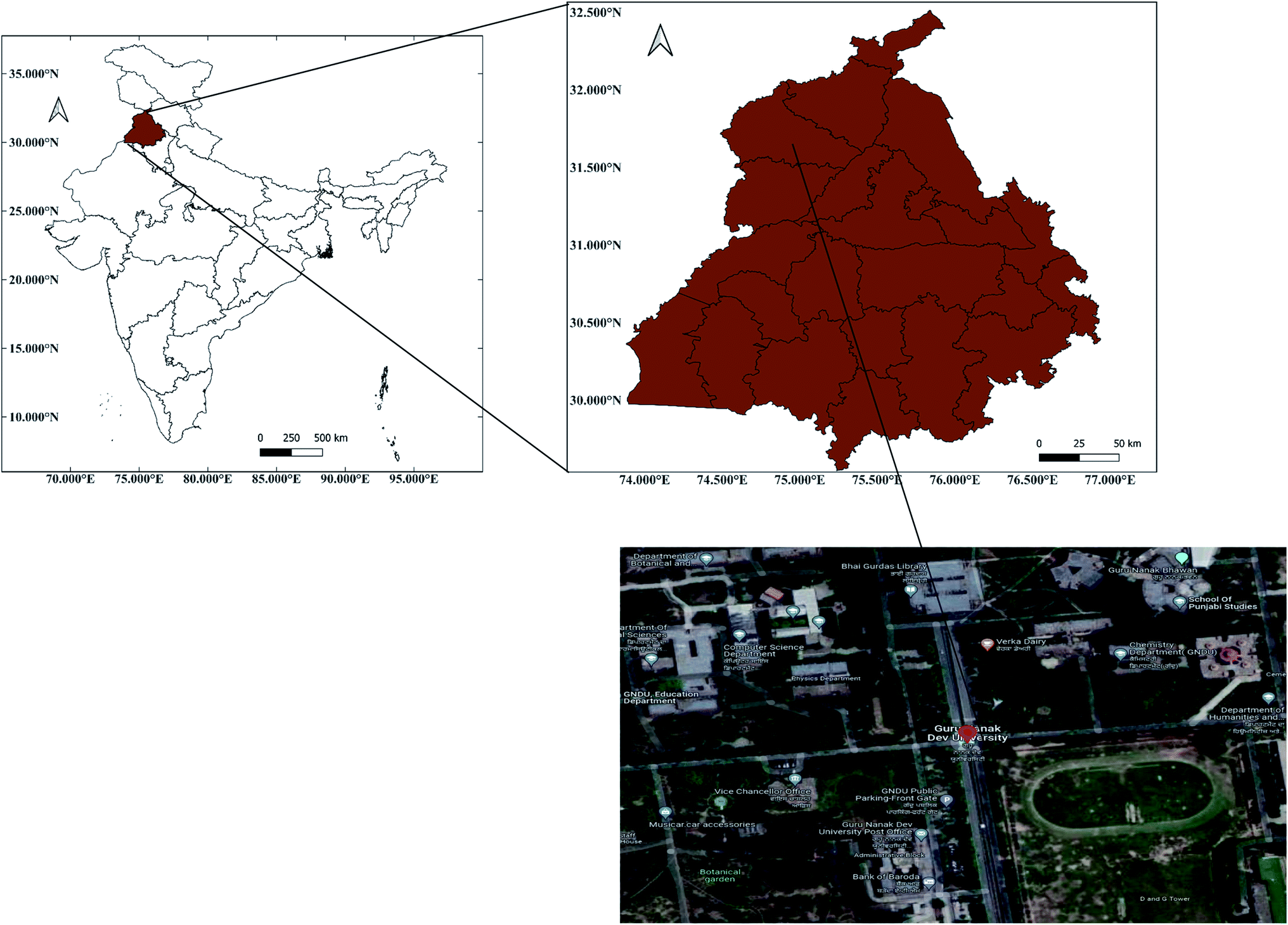
Fog samples were collected using indigenously fabricated glass collectors (0.5 m × 0.5 m) kept at the rooftop of an academic building in Guru Nanak Dev University, Amritsar, India having coordinates of 31.634°N and 74.872°E (Fig. 1 and S1†). The glass sheets were placed after sunset and samples were collected at sunrise. The samples volume below 25 ml were discarded. A sum of twenty fog samples was collected between November 2017 to February 2018 (Table S2†). The secondary data for air pollutants (PM_2.5, PM₁₀) and meteorological data (temperature, RH and visibility) was fetched from weather underground, the details of which are given in Yadav et al.¹⁷ Amritsar city is a holy city in the Amritsar district which forms a part of the IGP. Since a large number of pilgrims and tourists visit the holy city every day, vehicular movement within and around the city is quite large. In addition, agricultural residue burning in the after-harvest season (September and October) emits large amounts of pollutants to the atmosphere. Amritsar district experiences four seasons viz. (i) winter season (late November–March) (ii) hot season (April–June) (iii) southwestern monsoon season (early July-first week of September) and (iv) post-monsoon or transition period (late September–early November) with annual precipitation in the range of 500–600 mm. During the winter, there is near freezing temperature, and temperature inversion does not allow aerosol particles to escape, adding to the pollution load in the city. The western disturbances affect the weather during the winter season which is responsible for widespread rain and gusty winds.

Fig. 1 Map of sampling location.

2.2 Chemical analysis

All the samples were pre-filtered using 0.22 μm millipore membrane filter and immediately analysed for pH and electrical conductivity (EC). Samples were stored in polypropylene bottles at 8 °C for further analysis. Ion-chromatograph (Metrohm 883 Basic IC plus; Switzerland) equipped with a conductivity detector and Metrosep-A Supp 5–250/4.0 column was used for the analysis of anions. The mobile phase was a mixture of 3.2 mM sodium carbonate and 1 mM sodium bicarbonate solution at a flow rate of 0.7 ml min⁻¹. The retention time for Cl⁻, NO₃⁻ and SO₄²⁻ were 7.58, 12.53, 23.20 min, respectively and instrument calibration using sigma multi-ion standard curves gave a coefficient of determination (R²) close to 1.0 with overlay chromatograms shown in Fig. S2.†

2.3 Statistical analysis

Multiple regression analysis involves a set of statistical components in estimating the relationship between dependent and independent variables. This predicts the outcome of response variables on a set of independent variables. A statistical model has developed between two independent variables namely PM_2.5/PM₁₀ ratio and RH with visibility as a response variable. ANOVA model was generated using sequential model fitting for linear, two-factor interaction (2FI) and quadratic and the best model is proposed based on R², normal plot of the residual and box-cox plot for data transformation. Normal-plot of residuals indicates the distribution of residual errors in the model term. If all the data points do not lie along the straight line, then data transformation may help in improving the model fitting. After data passed the above test, MLR equations having RH and PM_2.5/PM₁₀ ratio as independent variables are generated to predict the visibility. Three-dimensional (3-D) contour plots are used to visualise the modelled data. Design-Expert software (Stat-Ease, Inc. Minneapolis, USA v. 13) was used for the statistical analysis.

3. Results and discussions

Fog samples were collected on the rooftop of the department of Guru Nanak Dev University and further characterised to understand its chemical composition. A sum of twenty samples was collected during the season on the inclined glass sheets (Table S2†).

3.1 Fog characterization

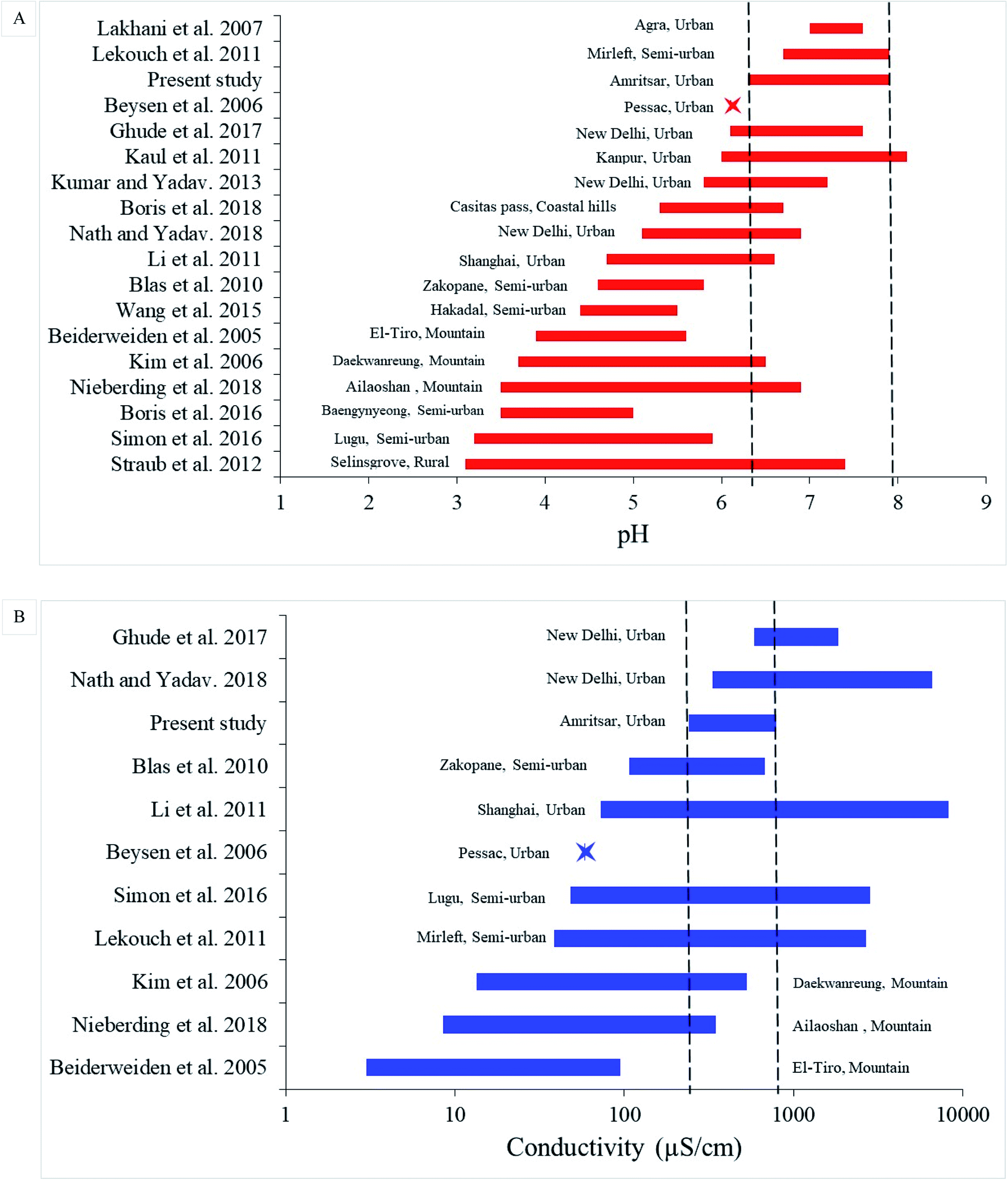
pH. pH is an intensity factor and a significant parameter to study the fog characteristics. The collected fog samples (n = 20) have pH ranges of 6.3–7.9 with an average value of 7.2 ± 0.4 (Table S2†). The frequency distribution of pH shows maximum samples are concentrated within 6.96–7.24 (Fig. S3a†). Other Indian urban cities (Agra, New Delhi and Kanpur) have shown pH ranging between 7 ± 1 (ref. 6, 27, and 28) whereas the majority of the international studies having rural and semi-urban background has pH as low as pH of 3.1.²⁹ Agriculture residue burning, vehicular transport emissions and long-range transport could be the reason for variation in pH in fog water (Fig. 2a).

Fig. 2 Global perspective of (A) pH and (B) conductivity measurements in fog water.

Electrical conductivity. EC of the collected samples ranged between 240–790 μS cm⁻¹ with an average value of 450 ± 14 μS cm⁻¹ (Table S2†). Most fog samples show lower EC i.e., 10 no of samples were within 240–420 μS cm⁻¹ and 8 no of samples are within 420–600 μS cm⁻¹ (Fig. S3b†). EC level of fog samples is compared with other sites as given in Fig. 2b. Megacity Delhi which is just 500 km away from the observational site has a higher conductivity range of 1236 μS cm⁻¹ (ref. 6) and 3501 μS cm⁻¹ (ref. 30) as compared to the present study. There are few studies on conductivity in fog water, which has indicated that inorganic constituents could be the correctness of analysis using ionic balance. The conductivity values are less than 100 μS cm⁻¹ at a few sites in Europe.^31,32 The minimum conductivity was found at a mountain site (at mean sea level: 2800 m) in Ecuador³³ and the highest value of 3500 μS cm⁻¹ was obtained for Shanghai (Fig. 2b), which has presented a wide range of conductivity.

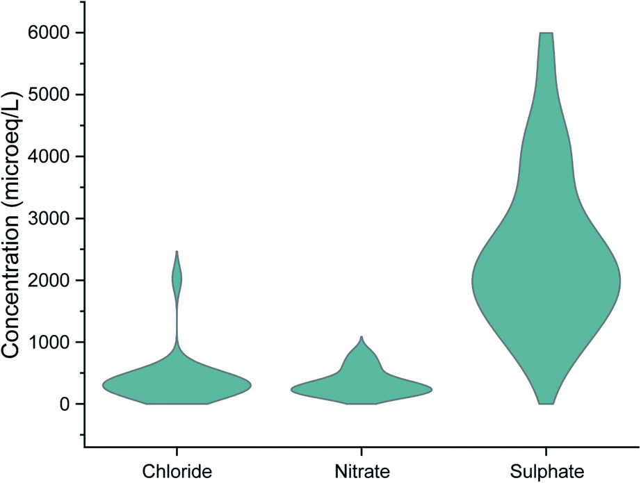
Chemical composition. Average anionic concentrations (μeq L⁻¹) in the present study were in the order of SO₄²⁻ > Cl⁻ > NO₃⁻ as shown in the violin plot (Fig. 3). Nath and Yadav³⁰ have also shown a similar sequence in the anionic concentration (SO₄²⁻ > Cl⁻ > NO₃⁻) in the fog samples over Delhi. The SO₄²⁻ concentration in the fog samples in the present study showed a wide range of variation (823–5642 μeq L⁻¹; average: 2465 ± 1243 μeq L⁻¹) with the minimum value on December 29, 2017, and maximum on January 5, 2018. Cl⁻ was the second most dominant ion (391 ± 401 μeq L⁻¹) found in the fog water in the present study. Like SO₄²⁻, the Cl⁻ (108–571 μeq L⁻¹) and NO₃⁻ (106–836 μeq L⁻¹) content in Amritsar also showed a very wide range. On December 29, 2017, Cl⁻ content in fog water over Amritsar was extremely high (2026 μeq L⁻¹) when SO₄²⁻ concentration (823 μeq L⁻¹) was low. The average concentration of NO₃⁻ in the fog water of Amritsar was 324 ± 216 μeq L⁻¹. The frequency distribution of Cl⁻ concentration showed that maximum fog events are concentrated within 200–400 μeq L⁻¹, whereas NO₃⁻ and SO₄²⁻ do not show any such trend. Table S1† shows the comparison of SO₄²⁻, Cl⁻, NO₃⁻ present in fog samples along with major sources of pollution with other sites across the globe. The concentration of SO₄²⁻ (823–5642) μeq L⁻¹ in fog water over Amritsar was among the top five locations exhibiting maximum SO₄²⁻ in comparison to other locations of the world. The highest SO₄²⁻ was found in New Delhi (887–40 653) μeq L⁻¹ followed by Shanghai (2830 μeq L⁻¹). The minimum concentration of SO₄²⁻ was found for Casitas Pass situated in the coastal hills followed by Norway and Ecuador (Fig. 4a). Sulphur dioxide in the ambient atmosphere acts as a precursor of sulphate. The atmospheric oxidation of SO₂ leads to the formation of sulphate which acts as an acidifying pollutant in the fog water.^34,35 Nath and Yadav³⁰ suggested agriculture fields, coal-fired power plants near the vicinity of the area, fossil fuel combustion, biomass burning as possible contributing sources over Delhi. Fig. 4b represents the comparison of the Cl⁻ content in fog water of Amritsar with other sites across the globe. Maximum Cl⁻ content (1716–16 109 μeq L⁻¹) was reported at southwestern Morocco, a semi-arid coastal area exhibiting marine origin³⁶ followed by New Delhi³⁰ and Taiwan.³⁴ The minimum was found in a mountain site in China.³² A major source of chloride in the environment is plastic burning. The other possible sources in the area could be the local emissions because of fabric bleaching activity in the nearby export garment factories (Table S1†). Industrial emissions may be a possible source contributing to Cl⁻ in the environment.³⁷ Fig. 4c compares the NO₃⁻ concentration in fog water of Amritsar with other sites across the globe and the dotted lines represent the reference range of ions in the present study. The highest NO₃⁻ concentration was found over Delhi as 253–15 787 μeq L⁻¹ followed by Shanghai.³⁸

Fig. 3 Violin plot showing the anions (μeq L⁻¹) in the fog water collected in Amritsar.

Fig. 4 Anionic concentration (μeq L⁻¹) of (A) sulphate (B) chloride (C) nitrate in fog water by different studies conducted worldwide.

During the winter season, pollutants get trapped by the lower PBL allowing maximum time to interact with the surrounding atmosphere³⁹ and higher concentration in the condensate samples. Over Amritsar, after crop harvesting (October and November), large crop residue or stubble is left over a vast area. To clear the area and prepare for the next sowing season, leftover biomass is burned every year elevating the concentration of the pollutant. The emission of sulphates and nitrate from biomass burning in agricultural fields may be abundant during this season around Amritsar.^40,41 Moreover, the emission of anions from vehicular exhaust over Amritsar, a holy city is quite significant.^36,42 The presence of excess sulphate and nitrate in fog water is linked to acidity.⁴³ Other than this biomass burning is a major factor that results in excess release of sulphates, nitrate, ammonium and sodium in the atmosphere.⁴⁴

3.2 Nitrate (NO₃⁻) to sulphate (SO₄²⁻) ratio in fog water

Table S1† shows the comprehensive view of the NO₃⁻ to SO₄²⁻ ratio along with the major contributing sources of the various locations conducted on a global scale. The observed nitrate to sulphate ratio was less than unity in the majority of sites except for three cases, where this ratio is greater than unity (Fig. 5). Previously reported studies were conducted in South Korea^41,45 USA,⁴⁶ Norway⁴⁷ and Taiwan³⁴ indicating vehicular emissions as a major contributor. Several researchers have also used NO₃⁻/SO₄²⁻ ratio as an indicator of the contribution of stationary and mobile sources.^34,48,49 In the present study, the NO₃⁻/SO₄²⁻ ratio in the fog samples ranged between 0.06–0.48 with an average of 0.15 ± 0.10 indicating an emission from fossil fuels (coal, pet coke) which is likely to be the emissions from coal-based thermal power plants located 40 km of the south-east of Amritsar and industrial clusters situated on the periphery of the city. It may not be the only reason as the majority of the time, the prevailing wind direction over Amritsar is northwest.¹⁷ Over Delhi, the NO₃⁻/SO₄²⁻ ratio was found to be 0.39, which was more than double as compared to Amritsar. Sulphate and nitrate concentrations over Delhi were found to be of the order of 40 000 μeq L⁻¹ and 15 000 μeq L⁻¹, respectively which could be the emissions from coal-fired power plants and particularly high-density automobile activity. At such a high value, the NO₃⁻/SO₄²⁻ ratio becomes unimportant. SO₄²⁻ and NO₃⁻ levels in the present study were around 5600 μeq L⁻¹ and 850 μeq L⁻¹, respectively, which is only about 10–20% of Delhi. Among the other sites of India, the NO₃⁻/SO₄²⁻ ratio was maximum at Agra (0.71), a city located about 200 km from New Delhi.²⁷ The highest ratio was for the USA (2.25) as reported by Boris et al.⁴⁶ indicating urban and industrial combustion, marine influence as major contributing factors followed by Norway (1.41).⁴⁷

Fig. 5 Stacked graph for nitrate and sulphate concentration (meq L⁻¹) along with nitrate to sulphate molar ratio in fog water. X-axis showing location (reference).

3.3 Statistical analysis

The ionic composition of fog water along with PM_2.5, PM₁₀ and PM_2.5/PM₁₀ ratio, RH and visibility data are tabulated in Table S2.† Various efforts were applied to develop the significant fitted model which can be used for predicting visibility as a response variable. No significant model was generated between pH, EC, Cl⁻, SO₄²⁻, NO₃⁻, ambient temperature with visibility for both individual model terms and in combinations with others except for the ratio of PM_2.5/PM₁₀ and RH with visibility.

In the present study, there are 17 data points during which heavy fog was witnessed and the PM_2.5/PM₁₀ ratio varied from (0.34 to 0.56) and RH varied between (71–97%). The average PM_2.5/PM₁₀ ratio (47%) of particulate matter load showed the abundance of finer particles (PM_2.5) in the ambient air. The minimum visibility (0.2 km) was on February 2, 2018, and the maximum of 4.3 km on December 13, 2017. The maximum visibility was observed when the contribution of PM_2.5 in the PM₁₀ ratio was minimum (0.34). The sequential ANOVA model suggested linear fit with skewed normal-plot of residuals. A large incremental change in visibility for a small change in PM_2.5/PM₁₀ ratio or RH and the significant difference between the maximum (4.3 km) to minimum (0.2 km) visibility, which was obtained as 21.5 (ratio greater than 10 indicates response transformation). Thus, the fitted model was checked using diagnostic plots with the help of Design-Expert software. Box-cox plot for power transformation recommended square root transformation (Fig. S4†). The model was again run after applying square root transformation which again suggested the multiple linear regression model as the best-fitted model. Diagnostic plots viz., the normal plot of residuals (Fig. S5†) indicated good model fitting. The Sequential ANOVA model suggested linear fit and the model was significant at F-value 41.64 with excellent model statistics (Table 1). Thus, a model can be navigated in design space and model equations are generated in coded (eqn (1)) and actual form (eqn (2)). The coded equation is used to check the relative importance of two independent variables. From eqn (1), the contribution of RH (unitless regression coefficient of −0.537) is more than PM_2.5/PM₁₀ ratio (unitless regression coefficient of −0.225). Although, both the variables showed negative effect on visibility as minimization of these two independent variables is the goal for maximisation of visibility. Under actual conditions, RH is an uncontrollable variable, but contribution of PM_2.5 in PM₁₀ can be minimised using better emission control measures to increase the visibility during foggy events.

(Visibility)^1/2 = 1.24 − 0.537 × RH − 0.225 × PM_2.5/PM₁₀ ratio, (1)

where, visibility in km and both independent variables viz. RH & PM_2.5/PM₁₀ ratios are in coded units. Coded values range between −1 (min) to +1 (max) and any other value within the model range is calculated using the concept of proportionality.

(Visibility)^1/2 = 5.632 − 0.041 × RH − 2.046 × PM_2.5/PM₁₀ ratio, (2)

where, visibility in km and RH (71–97%) & PM_2.5/PM₁₀ ratio (0.34–0.56) in actual units.

Table 1 ANOVA table and model statistics for the effect of PM_2.5/PM₁₀ ratio and relative humidity (RH) on visibility

Source	Sum of square	DoF^b	Mean square	F-Value	p-Value
a Significant at p ≤ 0.05.b Degree of freedom.
Model	3.31	2	1.65	41.64	<0.0001^a
RH	2.09	1	2.09	52.62	<0.0001^a
PM2.5/PM10	0.1902	1	0.1902	4.79	0.0461^a
Model statistics
Std. Dev.	0.199		R^2	0.856
Mean	1.18		adjusted R^2	0.835
C.V.%	16.86		predicted R^2	0.796

---

Fitted model equations are used to check the model fitting through predicted vs. actual plot (Fig. 6a). 3-D contour plot between PM_2.5/PM₁₀ ratio and RH with visibility (Fig. 6b) indicated maximisation of both PM_2.5/PM₁₀ ratio and RH for minimum visibility, but RH has a more profound effect on visibility as compared to PM_2.5/PM₁₀ ratio (Fig. S6†). Finally, an overlay plot was generated for visibility which indicated a PM_2.5/PM₁₀ ratio of 0.34 and RH > 95% or a PM_2.5/PM₁₀ ratio of 0.56 and RH > 85% as constraint conditions for forecasting visibility less than 1 km (Fig. 6c).

Fig. 6 Multiple regression fitted model for PM_2.5/PM₁₀ ratio and relative humidity (RH) on visibility (A) predicted vs. actual plot (B) 3-D contour plot (C) overlay plot (yellow colour) showing process conditions for PM_2.5/PM₁₀ ratio and RH for visibility less than 1 km.

In the absence of data points, the significance of the correlation coefficient cannot be defined as the degree of freedom is an important parameter for model fitting. Also, model fitting is done by splicing the data into different subsets like RH < 30%, RH > 70%. In the present study, visibility predictions were done using a proper statistical approach showing a normal plot of residuals and 3-dimensional contour plots to forecast the visibility.

4. Conclusions

The fog water was collected and characterised to evaluate the dominance of anions and to compare at the global level. The pH 7.2 ± 0.1 and EC 450 ± 50 μS cm⁻¹ was observed in the fog samples. The dominance of ions was in the order SO₄²⁻ > Cl⁻ > NO₃⁻. NO₃⁻/SO₄²⁻ ratio was found to be 0.15 indicating the dominance of sulphate emissions over nitrate. Multiple regression analysis of PM_2.5/PM₁₀ ratio and relative humidity with visibility indicated square root transformation of the visibility for the best fitted linear model. A multiple linear regression model for PM_2.5/PM₁₀ ratio and RH with visibility was developed and used for forecasting visibility. But RH has a more profound effect on visibility as compared to the PM_2.5/PM₁₀ ratio. Contour plot between PM_2.5/PM₁₀ ratio and RH vs. visibility and overlay plot may be helpful visualisation of the fitted model. Future studies can be directed to understand the complex relationship between PBL, wind profile, ventilation coefficient with the role of ultrafine particulate matter on reduced visibility.

Funding

This research did not receive any specific grant from funding agencies in the public, commercial, or not-for-profit sectors.

Data availability

All data generated or analysed during this study are included in the ESI† file of the submitted article.

Author contributions

The idea was conceptualised by M. S. B., who also devised the statistical test. R. Y. carried out all of the experiments and prepared the paper. A. S. helped in data curation. S. K. K., S. K. S. and T. K. M. assisted with data analysis, reviewing, proofreading and supervision.

Conflicts of interest

The authors declare no conflict of interest.

Acknowledgements

Authors are thankful to UGC-UPE supported Emerging Life Sciences, Guru Nanak Dev University, Amritsar, India for providing Ion-Chromatography. S. K. S. and T. K. M. are thankful to Director, CSIR-National Physical Laboratory (CSIR-NPL), New Delhi and Head of Environmental Sciences & Biomedical Metrology Division, CSIR-NPL for allowing to carry out the work.

References

1. The Global Risks Report 2022, Published by World Economic Forum ISBN, ISBN: 978-2-940631-09-4, 17th edn, https://www3.weforum.org/docs/WEF_The_Global_Risks_Report_2022.pdf.
2. N. Ojha, A. Sharma, M. Kumar, I. Girach, T. U. Ansari, S. K. Sharma, N. Singh, A. Pozzer and S. S. Gunthe, Sci. Rep., 2020, 10, 5862.
3. A. Sen, A. S. Abdelmaksoud, Y. N. Ahammed, M. A Alghamdi, T. Banerjee, M. A. Bhat, A. Chatterjee, A. K. Choudhuri, T. Das, A. Dhir, P. P. Dhyani, R. Gadi, S. Ghosh, K. Kumar, A. H. Khan, M. Khoder, K. M. Kumari, J. C. Kuniyal, M. Kumar, A. Lakhani, P. S. Mahapatra, M. Naja, D. Pal, S. Pal, M. Rafiq, S. A. Romshoo, I. Rashid, P. Saikia, D. M. Shenoy, V. Sridhar, N. Verma, B. M. Vyas, M. Saxena, A. Sharma, S. K. Sharma and T. K. Mandal, Atmos. Environ., 2017, 154, 200–224.
4. P. Sujatha, D. V. Mahalakshmi, A. Ramiz, P. V. N. Rao and C. V. Naidu, Cogent Environ. Sci., 2016, 2(1), 1125284.
5. Road accidents in India, report by Ministry of Road Transport and Highways, Government of India, 2017, p. 17, https://www.indiaenvironmentportal.org.in/files/file/road%20accidents%20in%20India%202017.pdf.
6. S. D. Ghude, G. S. Bhat, T. Prabhakaran, R. K. Jenamani, D. M. Chate, P. D. Safai, A. K. Karipot, M. Konwar, P. Pithani, V. Sinha, P. S. P. Rao, S. A. Dixit, S. Tiwari, K. Todekar, S. Varpe, A. K. Srivastava, D. S. Bisht, P. Murugavel, K. Ali, U. Mina, M. Dharua, Y. J. Rao, B. Padmakumari, A. Hazra, N. Nigam, U. Shende, D. M. Lal, B. P. Chandra, A. K. Mishra, A. Kumar, H. Hakkim, H. Pawar, P. Acharja, R. Kulkarni, C. Subharthi, B. Balaji, M. Varghese, S. Bera and M. Rajeevan, Curr. Sci., 2017, 112(4), 767–784.
7. I. Gultepe, R. Tardif, S. C. Michaelides, J. Cermak, A. Bott, J. Bendix, M. D. Muller, M. Pagowski, B. Hansen, G. Ellrod, W. Jacobs, G. Toth and S. G. Cober, Pure Appl. Geophys., 2007, 164(6), 1121–1159.
8. National Oceanic and Atmospheric Administration, Surface weather observations and reports, Federal Meteorological Handbook No. 1, 2017, p. 98, available from, U.S. Department of Commerce, NOAA, Office of the Federal Coordinator for Meteorological Services and Supporting Research, 1325 East-West highway suite 7130, Silver Spring, Maryland 20910 301-628-0112, accessed on August 20, 2020, https://www.ofcm.gov/publications/fmh/FMH1/FMH1_2017.pdf.
9. J. Quan, Q. Zhang, H. He, J. Liu, M. Huang and H. Jin, Atmos. Chem. Phys. Discuss., 2011, 11(4), 11911–11937.
10. Y. Zhu, Z. Li, F. Zu, H. Wang, Q. Liu, M. Qi and Y. Wang, Atmos. Res., 2022, 265, 105914.
11. Y. Gao and H. Ji, Chemosphere, 2018, 212, 346–357.
12. K. Ali, P. Acharja, D. K. Trivedi, R. Kulkarni, P. Pithani, P. D. Safai, D. M. Chate, S. Ghude, R. K. Jenamani and M. Rajeevan, Sci. Total Environ., 2019, 662, 687–696.
13. S. Kaur, K. Senthilkumar, V. K. Verma, B. Kumar, S. Kumar, J. K. Katnoria and C. S. Sharma, Arch. Environ. Contam. Toxicol., 2013, 65(3), 382–395.
14. S. Gulia, A. Shrivastava, A. K. Nema and M. Khare, Environ. Model. Assess., 2015, 20(6), 599–608.
15. S. Kumar, S. Nath, M. S. Bhatti and S. Yadav, Aerosol Air Qual. Res., 2018, 18(7), 1573–1590.
16. K. Ravindra, T. Singh, S. Mor, V. Singh, T. K. Mandal, M. S. Bhatti, S. K. Gahlawat, R. Dhankhar, S. Mor and G. Beig, Sci. Total Environ., 2019, 690, 717–729.
17. R. Yadav, M. S. Bhatti, S. K. Kansal, L. Das, V. Gilhotra, A. Sugha, D. Hingmire, S. Yadav, A. Tandon, R. Bhatti, A. Goel and T. K. Mandal, SN Appl. Sci., 2020, 2, 1761.
18. Y. Gu, H. Kusaka, V. Q. Doan and J. Tan, Atmos. Res., 2019, 220, 57–74.
19. S. Tiwari, S. Payra, M. Mohan, S. Verma and D. S. Bisht, Atmos. Pollut. Res., 2011, 2(1), 116–120.
20. T. Luan, X. Guo, L. Guo and T. Zhang, Atmos. Chem. Phys., 2018, 18(1), 203–225.
21. X. Wang, R. Zhang and W. Yu, J. Geophys. Res.: Atmos., 2019, 124(4), 2235–2259.
22. P. D. Safai, S. Ghude, P. Pithani, S. Varpe, R. Kulkarni, K. Todekar, S. Tiwari, D. M. Chate, T. Prabhakaran, R. K. Jenamani and M. N. Rajeevan, Aerosol Air Qual. Res., 2019, 19(1), 71–79.
23. W. S. Won, R. Oh, W. Lee, K. Y. Kim, S. Ku, P. C. Su and Y. J. Yoon, Aerosol Air Qual. Res., 2020, 20(5), 1048–1061.
24. J. Chen, S. Qiu, J. Shang, O. M. Wilfrid, X. Liu, H. Tian and J. Boman, Aerosol Air Qual. Res., 2014, 14(1), 260–268.
25. Y. Yang, B. Ge, X. Chen, W. Yang, Z. Wang, H. Chen, D. Xu, J. Wang, Q. Tan and Z. Wang, Atmos. Res., 2021, 256, 105565.
26. Z. Liu, H. Wang, Y. Peng, W. Zhang and M. Zhao, Atmosphere, 2022, 13(2), 203.
27. A. Lakhani, R. S. Parmar, G. S. Satsangi and S. Prakash, Environ. Monit. Assess., 2007, 133(1), 435–445.
28. D. S. Kaul, T. Gupta, S. N. Tripathi, V. Tare and J. L. Collett Jr, Environ. Sci. Technol., 2011, 45(17), 7307–7313.
29. D. J. Straub, J. W. Hutchings and P. Herckes, Atmos. Environ., 2012, 47, 195–205.
30. S. Nath and S. Yadav, Aerosol Air Qual. Res., 2018, 18, 26–36.
31. D. Beysens, C. Ohayon, M. Muselli and O. Clus, Atmos. Environ., 2006, 40(20), 3710–3723.
32. F. Nieberding, B. Breuer, E. Braeckevelt, O. Klemm, Q. Song and Y. Zhang, Aerosol Air Qual. Res., 2018, 18, 37–48.
33. E. Beiderwieden, T. Wrzesinsky and O. Klemm, Hydrol. Earth Syst. Sci., 2005, 9, 185–191.
34. S. Simon, O. Klemm, T. El-Madany, J. Walk, K. Amelung, P. H. Lin, S. C. Chang, N. H. Lin, G. Engling, S. C. Hsu, T. H. Wey, Y. N. Wang and Y. C Lee, Aerosol Air Qual. Res., 2016, 16, 618–631.
35. J. Suneja, G. Kotnala, A. Kaur, T. K. Mandal and S. K. Sharma, Mapan, 2020, 35(1), 125–133.
36. I. Lekouch, M. Muselli, B. Kabbachi, J. Ouazzani, I. Melnytchouk-Milimouk and D. Beysens, Energy, 2011, 36(4), 2257–2265.
37. K. Ali, G. A. Momin, S. Tiwari, P. D. Safai, D. M. Chate and P. S. P. Rao, Atmos. Environ., 2004, 38(25), 4215–4222.
38. P. Li, X. Li, C. Yang, X. Wang, J. Chen and J. L. CollettJr, Atmos. Environ., 2011, 45(24), 4034–4041.
39. A. Sen, T. K. Mandal, S. K. Sharma, M. Saxena, N. C. Gupta, R. Gautam, A. Gupta, T. Gill, S. Rani, T. Saud, D. P. Singh and R. Gadi, Atmos. Environ., 2014, 99, 411–424.
40. T. Saud, T. K. Mandal, R. Gadi, D. P. Singh, S. K. Sharma, M. Saxena and A. Mukherjee, Atmos. Environ., 2011, 45(32), 5913–5923.
41. A. J. Boris, T. Lee, T. Park, J. Choi, S. J. Seo and J. L. Collett Jr, Atmos. Chem. Phys., 2016, 16(2), 437–453.
42. P. Kumar and S. Yadav, Environ. Monit. Assess., 2013, 185(3), 2795–2805.
43. M. Błaś, Z. Polkowska, M. Sobik, K. Klimaszewska, K. Nowiński and J. Namieśnik, Atmos. Res., 2010, 95(4), 455–469.
44. Saraswati., S. K. Sharma, M. Saxena and T. K. Mandal, Atmos. Res., 2019, 218, 34–49.
45. M. G. Kim, B. K. Lee and H. J. Kim, J. Atmos. Chem., 2006, 55(1), 13–29.
46. A. J. Boris, D. C. Napolitano, P. Herckes, A. L. Clements and J. L. Collett Jr, Aerosol Air Qual. Res., 2018, 18, 224–239.
47. Y. Wang, J. Zhang, A. R. Marcotte, M. Karl, C. Dye and P. Herckes, Atmos. Res., 2015, 151, 72–81.
48. D. Migliavacca, E. C. Teixeira, F. Wiegand, A. C. M. Machado and J. Sanchez, Atmos. Environ., 2005, 39(10), 1829–1844.
49. A. Agarwal, A. Satsangi, A. Lakhani and K. M. Kumari, Chemosphere, 2020, 242, 125132.

---

Footnotes

† Electronic supplementary information (ESI) available. See https://doi.org/10.1039/d2ra00424k

‡ Contributed equally.

---