Machine learning based on structural and FTIR spectroscopic datasets for seed autoclassification

Abstract

A single feature set is often unable to effectively classify complex biological samples due to their similar morphology and sizes. This paper proposes a protocol for the fast identification of seed medicinal materials based on micro-structural and infrared spectroscopic characteristics. Three different feature datasets, namely micro-CT, FTIR, and mixed datasets, were established via principal component analysis (PCA) and competitive adaptive reweighted sampling (CARS) and then used to train a back-propagation neural network. The mixed dataset consists of 34-dimensional micro-CT eigenvalues and 13-dimensional FTIR eigenvalues, optimized by PCA and CARS processing and then used to train a BP neural network. The results showed that the classification accuracy reached 89.5% for the micro-CT dataset and 93.3% for the FTIR dataset, and the classification accuracy of the mixed dataset achieved 99.2%, much higher than those of the traditional single feature datasets. This study provides a new protocol for multi-dimensional characteristic architecture with excellent performance for the classification and identification of Chinese medicinal materials.

---

1 Introduction

Seeds are widely used in herbal medicine and play an important role in traditional Chinese medicine (TCM). However, seeds are huge in number as well as in species, and many are named even for the same species. Furthermore, many seeds are similar in shape, appearance, size and internal structure, especially those from homologous genera of plants. There are many seeds not documented in the Chinese pharmacopoeia in a standardized manner, hampering their classification and usage. This can lead to confusion and misuse of seed herbs and even cause the emergence of fake herbs. Therefore, it is necessary to develop a rapid identification tool for herbs using multi-dimensional intelligent methods.

Current medical botanical identification is mainly based on imaging, spectroscopic, and biochemical techniques as well as manual classification. For example, the identification of six species of Litsea Lam by scanning electron microscopy,¹ establishment of the spectral fingerprint of Swertia mileensis for its quality control,² identification of ginseng from China and Korea by isotope tracing,³ and identification of fake Semiaquilegia adoxoides by biomolecular methods.⁴ However, these methods are costly and need complex sample preparation and handling procedures. Infrared spectroscopic techniques such as visible/near-infrared spectroscopy (VIS/NIR), near-infrared spectroscopy (NIR), mid-infrared spectroscopy (MIR), and hyperspectral imaging (HSI) can be used to analyse the species and places of origin of plants. For instance, VIS/NIR is used to distinguish crop growing regions and detect nutritional indicators.^5,6 Since the spectra contain chemical information about the plant, they can reflect differences in the spectra of plants of different varieties and geographical origin, such as in food quality testing using spectroscopic methods.^7,8 X-ray computed microtomography (CT) is a fast, non-destructive, multi-scale testing technique widely used in botany, biomedicine, food testing and security. For example, the identification of New Zealand plant leaf material from artefacts using micro-computed micro-CT,⁹ imaging of mouse heart using micro-CT and eXIA-160 contrast agents,¹⁰ study of micro-deformations of breadcrumbs under severe compression,¹¹ testing of cellular food products,¹² and investigation of food microstructure evaluation.¹³ Due to the combination of high brightness, adjustable energy of synchrotron radiation and micro-CT, high-resolution 3-dimensional X-ray phase contrast imaging techniques are being increasingly employed in plant physiology and in situ structural identification. For example, cavitation and water recharge processes in rice and bamboo leaves were investigated successfully,¹⁴ feature tissues and calcium oxalates of wild ginseng were revealed,^15,16 and a phase-attenuation-duality-based phase retrieval algorithm effectively improved the density resolution of weakly absorbing materials and successfully visualized the morphological characteristics of eaglewood specimens at different stages.^17,18

Machine learning can solve real-world problems by extracting various features based on imaging, such as gray level co-occurrence matrix (GLCM), gray gradient co-occurrence matrix (GGCM) and Tamura texture values,^19,20 mass spectrometry, and chromatography.²¹ Recently, it has been introduced to medical botanical identification and classification, such as in the identification of bitter almond and peach kernel herbs of different origins using neural networks,²² the identification of licorice using support vector machines (SVMs) and random forests,²³ and the accuracy comparison of different classifiers of plant specimens.²⁴ Principal component analysis (PCA) is always used as a dimension reduction tool for machine learning, and can significantly reduce the time required for machine learning.

In this study, we propose a new protocol to develop a multi-dimensional intelligent method for identifying highly similar seed herbs. A mixed feature dataset was established using a combination of micro-CT structural and FTIR spectroscopic eigenvalues optimized by PCA and competitive adaptive reweighted sampling (CARS) methods,²⁵ including, GLCM, GGCM and Tamura texture values, and the FTIR vibration absorption feature peak (VAFP) technique. Then, a classifier based on a BP neural network was introduced and trained. The classification accuracy of the mixed dataset is much higher than that of the traditional dataset. This protocol has great potential in dealing with other problems of classification in medical botany.

2 Materials and methods

2.1 Preparations of samples

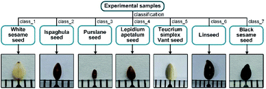
7 types of seeds with similar appearance, shown in Fig. 1, were used as our experimental samples at room temperature, provided by the Institute of Traditional Chinese Medicine and Ethnomedicine, Xinjiang Uyghur Autonomous Region. The encapsulated samples were first subjected to SR-XPCT experiments and after their 3D morphological data had been acquired, the sealed samples were treated with cutting and other processes and used for infrared data acquisition. For SR-XPCT data collection, the samples were not pre-treated in any way, such as cutting or staining, and placed in a conical transparent container and kept in a fixed position to avoid generating motion artifacts. Then, the samples were soaked for 6–8 hours and embedded, frozen at −24 °C and 7 μm thick slices with a frozen slicer (Leica CM3050 S) were obtained. The slices were carefully attached to BaF₂ substrates to improve their transmittance.

Fig. 1 Experimental samples of the 7 species of seeds.

2.2 Data collection

Our experiments were carried out using high-brightness synchrotron radiation to achieve high signal-to-noise ratio data at the Shanghai Synchrotron Radiation Facility (SSRF). To obtain the 3D morphological data, synchrotron-based X-ray phase contrast tomography (SR-XPCT) was employed to collect sample projections on a BL13HB beamline equipped with a CMOS camera with a resolution of 1.625 μm per pixel. The sample was placed in the centre of a rotary table to obtain the best results for reconstruction. The experimental conditions of SR-XPCT were as follows: photon energy 15 keV, sample-to-detector 80 mm, exposure time 1000 ms and 1080 projections per sample with 2048 × 2048 pixels. All SR-XPCT projections were pre-processed by background correction and phase retrieval to improve the density resolution of weakly absorbing samples, then reconstructed by filtered back-projection (FBP). The SR-FTIR data of 5 μm slices of each seed sample were collected in the transmission mode on the BL06B beamline at SSRF, equipped with a Nicolet 6700 FTIR spectrometer and Nicolet Continuμm Microscope. The conditions of FTIR mapping were as follows: 40 × 40 μm aperture, step size 40 μm, repeated times 8 in ROIs and 32 in background to ensure data reliability and a wavenumber range of 650–4000 cm⁻¹. The mapping area covered each entire seed slice. The VAFPs of each seed were processed and averaged with 30 points using the OPUS software.

The post-processing sample data were collected via feature extraction, combination and classification as shown in the flow diagram in Fig. 2. Both modality datasets were compared quantitatively. For the SR-XPCT dataset, the structural features were extracted via the GLCM, GGCM and Tamura texture methods. For the SR-FTIR dataset, the spectral features of the VAFPs were obtained through the CARS method, which is applied to the selection of the optimal subset of wavelengths. Its workflow usually includes four successive steps: Monte Carlo model sampling, forced wavelength reduction by an exponential decrement function (EDF), adaptive re-weighted sampling (ARS), and calculation of RMSECV for each subset. The mixed feature dataset was built based on both modality features and optimized by PCA.

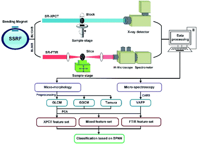Fig. 2 Schematic diagram of the multi-dimensional sample data acquisition and analysis system based on SR-XPCT and SR-FTIR in SSRF and the experimental flow chart.

2.3 Machine learning

Three feature datasets were trained and compared by a back-propagation neural network (BPNN), which is a multilayer feed-forward neural network with unidirectional transmission topology, consisting of an input layer, hidden layer and output layer. It is capable of learning and storing a large number of input–output pattern mappings. Using a gradient descent algorithm, it can achieve continuous adjustment of the weights of the network until the squared error is minimized.

A 3-layer BPNN (input, hidden, output layers) was introduced in this study, characterized by its compact structure to avoid long training time and the tendency of overfitting. The nodes of the hidden layer were essential to the accuracy of classification, and can be determined by the formula , where h is the number of nodes in the hidden layer, m and n are the number of nodes in the input and output layers, respectively, and a is the adjusting constant integer between 1 and 10. In this study, the number of nodes in the hidden layer was 11, and three feature datasets (SR-XPCT, SR-FTIR, mixed feature datasets) were used to train our BPNN adopt software Weka (version 3.6.15). Here, 70%, 15%, and 15% randomly selected points were applied for the training set, test set and validation set, respectively. The performance of BPNN was evaluated with four assessment criteria, as shown in Table 1. TP, TN, FP and FN represent true positive, true negative, false positive and false negative, respectively. Accuracy is the most intuitive performance measurement. It is the ratio of the number of correctly predicted samples to the total number of samples. Precision is the ratio of correctly predicted positive samples to the total predicted positive samples. Recall rate is the ratio of correctly predicted positive samples to all actual positive samples. F1 is a weighted average of precision and recall. The closer this value is to 1, the more accurate the model's predictions.

Table 1 Binary prediction models for classifiers and the assessment criteria

Real type	Predict type		Assessment criteria
	Positive	Negative	Accuracy	Precision	Recall	F1
Positive	TP	FN
Negative	FP	TN

---

3 Result

3.1 Dual modality dataset and feature architecture

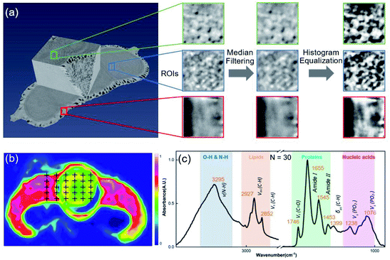
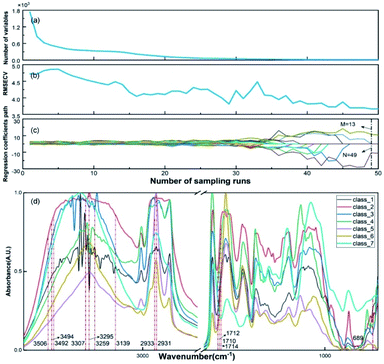
All SR-XPCT data of the seed samples were three-dimensionally reconstructed to extract the structural features using the pre-processing flow, as shown in Fig. 3(a). Sub-images of ROIs were chosen in three different regions, namely the cotyledon, embryo and seed coat areas, and then processed with median filter and histogram equalization to improve the signal-to-noise ratio and contrast of the image. Their eigenvalues were calculated by GLCM (16-dimensional features), GGCM (15-dimensional features) and Tamura texture (3-dimensional features). A 34-dimensional feature set was finally minimized into a 5-dimensional one using the PCA method, as shown in Fig. 5(a). SR-FTIR data of the seed slices was collected by mapping in the range of 650–4000 cm⁻¹ and processed via background subtraction, baseline correction, smoothing and averaging, as shown in Fig. 3(b). The VAFPs of biomacromolecules, including lipids, proteins, nucleic acids, and various chemical bonds, were determined by averaging of multiple points (N = 30), as shown in Fig. 3(c). Therefore, there are 1737 spectral channels used for building the SR-FTIR feature sets.

Fig. 3 Morphological and spectroscopic experimental results and data processing. (a) 3D rendering of the reconstruction of a seed sample and its image pre-processing flow. Green, blue, and red rectangles denote the embryo, cotyledon, and seed coat regions, respectively. (b) SR-FTIR mapping image of the sample in the 1500–1700 cm⁻¹ range, showing the distribution of proteins. VAFPs were measured at 30 points, indicated by cross symbols, to obtain the average spectrum. (c) Different feature peaks of biomacromolecules in the range of 4000–650 cm⁻¹.

The CARS method was employed to obtain the optimal variable number (M) of VAFPs using an iterating algorithm, as shown in Fig. 4(a). The number of sampling runs (N) can be effectively determined through the calculation of the lowest RMSECV value. In this study, the initialization parameters of CARS are A = 10 (maximum number of principal components), K = 10 (k-fold cross-validation), and N = 50 (maximum number of Monte Carlo sampling runs). The values of RMSECV fluctuated and approached zero at a given N, as shown in Fig. 4(b). The regression coefficient path reflected the optimal course of the eigenvalue number with increasing number of sampling runs, as shown in Fig. 4(c). The results of the CARS analysis showed that the RMSECV was minimal when the iteration proceeded to the 49th iteration, at which time there were 13 points with high specificity. It can be seen that CARS enabled the optimization of the data model, especially in increasing the identification of similarly structured samples. Fig. 4(d) presents the FTIR spectroscopic distribution and selected eigenvalues of the 7-species VAFPs.

Fig. 4 Calculation results of the CARS method. (a) The number of variables, (b) RMSECV and (c) regression coefficients of each variable with increasing number of sampling runs. (d) FTIR eigenvalues of 7 species of seed samples extracted from VAFPs.

The mixed feature dataset was built by the combination of both SR-XPCT and SR-FTIR optimal eigenvalues. The PCA method was applied to optimize the SR-XPCT and mixed feature sets to 5-dimensional and 8-dimensional feature sets, respectively, as shown in Fig. 5(a). Fig. 5(b) and (c) reflect the results of selected PCAs and data concentration, respectively, for the XPCT and mixed feature datasets. After PCA processing, the data in the mixed dataset were richer than those in the SR-XPCT dataset. The data in the CT dataset were more scattered, with large data overlap between classes, which made correct classification difficult. The data in the mixed dataset were more easily distinguishable due to the greater concentration of data. The numbers of three statistical samples are listed in Table 2. The total number of samples was 6642, and a total of 4650 samples were randomly selected from each species as the training set, 996 as the validation set, and 996 as the test set.

Fig. 5 Analytical results of the PCAs and the distribution for the SR-XPCT dataset and mixed dataset. (a) Individual and cumulative proportions of both PCAs; covered variance is set to 90%; (b) 5-dimensional principal components for the SR-XPCT dataset; (c) 8-dimensional principal components for the mixed dataset.

Table 2 Numbers of dataset of seeds for each species. A, B, and C represent the training set, validation set and test set, respectively

Class name	SR-XPCT			SR-FTIR			Mixed
	A	B	C	A	B	C	A	B	C
Class_1	750	125	125	740	130	130	730	135	135
Class_2	609	136	136	601	140	140	631	125	125
Class_3	664	168	168	670	165	165	676	162	162
Class_4	494	120	120	502	116	116	498	118	118
Class_5	685	161	161	685	161	161	719	144	144
Class_6	754	133	133	748	136	136	706	157	157
Class_7	694	153	153	704	148	148	690	155	155

---

3.2 Classification results based on BPNN

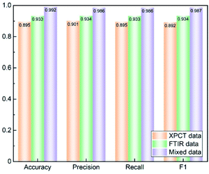
Three datasets were trained by BPNN with 11 nodes in 1 hidden layer, a learning rate of 0.3, momentum of 0.2 and 500 training times, and the results of accuracy, precision, recall and F1 are shown in Fig. 6. The SR-FTIR dataset got higher scores than the SR-XPCT dataset due to the highly similar image feature sites. The mixed dataset combined the advantages of the SR-XPCT and SR-FTIR datasets, and achieved a higher classification result. Such a high accuracy of classification is due to the small number of seed samples and seed species; the accuracy will decrease when the number and species of samples increase. For training complex samples, the classification accuracy of the mixed dataset is superior to that of traditional single datasets.

Fig. 6 Comparison of the classification performances of the SR-XPCT, SR-FTIR and mixed data models. The orange, green and purple bars represent the XPCT dataset, FTIR dataset and mixed dataset, respectively.

4 Discussion

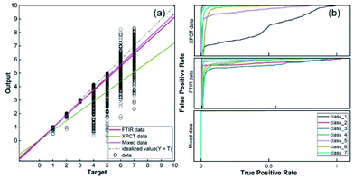
To demonstrate the advantages of mixed datasets over traditional datasets, radar plots and box line plots were prepared to represent the attributes and data distribution, respectively, of the SR-XPCT and mixed datasets. The area of the mixed dataset was larger than that of the SR-XPCT dataset, indicating that the mixed dataset contains more feature information to improve the accuracy of classification, as shown in Fig. 7(a). Fig. 7(b) and (c) reflect the data distribution of different species of samples in the SR-XPCT and mixed datasets, respectively. There is an obvious overlap between the means and medians of the various categories in the SR-XPCT dataset, which results in a lower accuracy of classification, whereas in the mixed dataset, the data overlap is lower, greatly improving the accuracy.

Fig. 7 Comparison of the SR-XPCT and mixed feature datasets. (a) Three metrics of performance represented by radar plots; (b) PCA data distribution of the SR-XPCT dataset; (c) PCA data distribution of the mixed dataset.

For further assessment of the classification performance of the three datasets, the method of regression analysis was employed in this study to analyse the relationship between dependent variables and independent variables by way of mathematical expression. As shown in Fig. 8(a), the regression values of the SR-XPCT, SR-FTIR and mixed dataset were 0.849, 0.956 and 0.969, respectively. The regression value of the SR-FTIR dataset was significantly higher than that of the SR-XPCT dataset, indicating that the classification performance of the SR-FTIR dataset was better. The regression line for the mixed dataset, closest to the idealized value, reflected that the trained results of the mixed dataset model had the clearest mapping to the true species. Receiver operating characteristic curves (ROCs) are generally used to evaluate the classification results of machine learning. The test results of the three datasets were calculated by ROC, as shown in Fig. 8(b). There are misclassifications between each species in both the SR-SPCT and SR-FTIR datasets due to insufficient discrimination using features of one single attribute, such as for class_1 and class_5 in the SR-XPCT dataset. Their structural features are so similar that their classification accuracies become relatively low. Moreover, the SR-FTIR dataset also suffers from the similarity problem, although the average accuracy is higher than that of the SR-XPCT dataset. This suggested that we need to combine more different attribute features into the optimal feature dataset to further discriminate similar and complex samples. Therefore, the mixed feature dataset was proposed for the autoclassification of seed samples. In comparison with the above datasets, the ROC of the mixed dataset exhibited better accuracy of classification (up to 99.2%). This demonstrated that a multi-attribute feature dataset can effectively improve the accuracy of classification for complex specimens, especially for biological samples. Indeed, multi-dimensional imaging methods have great potential in providing sufficient raw feature data for the identification of complex systems, combining the methods of feature extraction, PCA, and classifiers.

Fig. 8 Performance analysis of the three datasets. (a) Regression values for the SR-XPCT, SR-FTIR, and mixed datasets, with data points indicating the error between the target classification and the output value; (b) ROCs for the SR-XPCT, SR-FTIR, and mixed datasets.

Since confusion matrixes allow us to obtain the specific number of misclassifications, the confusion matrixes of the three types of datasets are shown in Fig. 9. In the SR-XPCT dataset, class_1 and class_5 had a much higher number of misclassifications compared to the other species, as illustrated in Fig. 8(b), which demonstrated that the similarity of microstructural features affects the accuracy of classification. For the SR-FTIR dataset, class_2, class_3, class_4 and class_6 were easily confused; this result was complementary to that of the SR-XPCT dataset and suggested that an approach combining microscopic and spectroscopic features was feasible. Our mixed dataset combining two features demonstrates this approach, and all species can be distinguished with high accuracy. Taking advantage of the complementary properties between different features, the mixed dataset is superior in identifying samples of similar species.

Fig. 9 Confusion matrixes for the SR-XPCT (a), SR-FTIR (b), and mixed (c) datasets; the green cells denote the correct number of classifications, red cells denote the incorrect number, and blue cells denote the rate of correct classification. The black percentages indicate the number of samples in the current grid as a percentage of the test set. The green and red numbers indicate the correct and incorrect classification rates for a category, respectively.

5 Conclusions

In this study, SR-XPCT and SR-FTIR datasets were combined to obtain a mixed dataset with machine learning to classify seed samples accurately. In this regard, a BPNN classifier was used to train the three datasets separately. Compared to the SR-XPCT or SR-FTIR datasets, the mixed dataset shows great superiority in classifying similar and complex samples. This protocol can also be applied to the identification of similar and complex characteristics in medicinal botany and biology. For samples with significant morphological or spectroscopic characteristics, classification can be performed using either a SR-XPCT or SR-FTIR feature set to save time.

Funding

This work was supported by the National Natural Science Foundation of China (Grant No. 12175127), Natural Science Foundation of Shandong Province, China (Grant No. ZR2020MA088) and Natural Science Foundation of Xinjiang Uygur Autonomous Region, China (Grant No. 2019D01C188).

Author contributions

Hanqiu Wang, Aybek Rehmetulla: methodology, experiments, writing – original draft. Shanshan Guo, Xin Kong, Zhiwei Lü, Yu Guan, Cong Xu: data process and analysis. Kaiser Sulaiman: experimental sample support and analysis. Gongxiang Wei, Huiqiang Liu: supervision, validation, writing – review and editing, funding acquisition.

Conflicts of interest

There are no conflicts to declare.

Acknowledgements

We thank the staff of the BL13HB beamline of the X-ray Imaging and Biomedical Application, BL06B beamline of Dynamic Beamline: IR Branch at the Shanghai Synchrotron Radiation Facility (SSRF), and BL01B beamline of the National Facility for Protein Science in Shanghai (NFPS) for their assistance during data collection.

References

1. Y. Chen, Dr thesis, Chengdu University of TCM, 2004.
2. F. Z. Aien Tao, Q. Chen and C. Xia, Dali Xueyuan Xuebao, 2020, 5(12), 27–31.
3. S. M. Choi, H. S. Lee, G. H. Lee and J. K. Han, Food Chem., 2008, 108, 1149–1154.
4. F. L. Shaotong Chen, Q. Zhao and B. Han, Lishizhen Medicine And Materia Medica Research, 2019,  DOI:10.3969/j.issn.1008-0805.2019.04.036.
5. W. Meulebroeck, B. Culshaw, H. Thienpont, A. G. Mignani, H. Bartelt and L. R. Jaroszewicz, presented in part at the Optical Sensing II, 2006.
6. A. G. Mignani, S. K. Khijwania, L. Ciaccheri, B. D. Gupta, B. P. Pal, A. A. Mencaglia and A. Sharma, presented in part at the Photonics 2010: Tenth International Conference on Fiber Optics and Photonics, 2010.
7. W. F. M. Yukihiro Ozaki and A. A. Christy, Near-Infrared Spectroscopy in Food Science and Technology, 2006.
8. A. Nawrocka and J. Lamorsk, in Advances in Agrophysical Research, 2013, ch. 14,  DOI:10.5772/52722.
9. C. Smith, B. Lowe, K. Blair, D. Carr and A. McNaughton, Stud. Conserv., 2013, 58, 256–268.
10. J. R. Ashton, N. Befera, D. Clark, Y. Qi, L. Mao, H. A. Rockman, G. A. Johnson and C. T. Badea, Contrast Media Mol. Imaging, 2014, 9, 161–168.
11. S. Guessasma and H. Nouri, Food Res. Int., 2015, 72, 140–148.
12. K. S. Lim and M. Barigou, Food Res. Int., 2004, 37, 1001–1012.
13. A. Léonard, S. Blacher, C. Nimmol and S. Devahastin, J. Food Eng., 2008, 85, 154–162.
14. Y. Xue, Dr thesis, Shanghai Institute of Applied Physics, Chinese Academy of Sciences, 2010.
15. L. Ye, Y. Xue, Y. Wang, J. Qi and T. Xiao, J. Ginseng Res., 2017, 41, 290–297.
16. Y. X. Linlin Ye, H. Tan, R. Chen, J. Qi and T. Xiao, Guangxue Xuebao, 2013, 12, 365–370.
17. H. Liu, F. Lin, J. Lin, K. Sulaiman, T. Xiao, Y. Sun, Y. Pang and H. Liu, Wood Sci. Technol., 2018, 52, 839–854.
18. S. K. Huiqiang Liu, Y. Sun, P. Yuan, X. Fan, R. Xie, C. Liu, Y. Duan and Y. Ma, Zhiwuxue Tongbao, 2018, 53(3), 364–371.
19. K. Chen, Y. Wang, P. Zhao, L. E. Banta and X. Zhao, J. Electron., 2009, 26, 428–432.
20. M. Hideyuki Tamura, S. Mori and T. Yamawaki, IEEE Transactions on Systems, Man, and Cybernetics: Systems, 1978.
21. F. Lussier, V. Thibault, B. Charron, G. Q. Wallace and J.-F. Masson, TrAC, Trends Anal. Chem., 2020, 124, 115769.
22. R. C.-l. Zheng Jie, Z. Lu, Y. I. N. Wen-Jun, Z. Hui and Y. A. N. Ji-Zhong, Zhongguo Zhongyao Zazhi, 2021, 46(10), 2571–2577.
23. R. C.-l. Yin Wen-Jun, Z. Jie, Z. Lu, Y. A. N. Ji-Zhong and Z. Hui, Zhongguo Zhongyao Zazhi, 2021, 46(4), 923–930.
24. D. Bambil, H. Pistori, F. Bao, V. Weber, F. M. Alves, E. G. Gonçalves, L. F. de Alencar Figueiredo, U. G. P. Abreu, R. Arruda and I. M. Bortolotto, Environ. Syst. Decis., 2020, 40, 480–484.
25. H. Li, Y. Liang, Q. Xu and D. Cao, Anal. Chim. Acta, 2009, 648, 77–84.

---

Footnote

† Equal contributors.

---