Supervised dimension reduction for optical vapor sensing

Abstract

Detecting and identifying vapors at low concentrations is important for air quality assessment, food quality assurance, and homeland security. Optical vapor sensing using photonic crystals has shown promise for rapid vapor detection and identification. Despite the recent advances of optical sensing using photonic crystals, the data analysis method commonly used in this field has been limited to an unsupervised method called principal component analysis (PCA). In this study, we applied four different supervised dimension reduction methods on differential reflectance spectra data from optical vapor sensing experiments. We found that two of the supervised methods, linear discriminant analysis and least-squares regression PCA, yielded better interclass separation, vapor identification and improved classification accuracy compared to PCA.

---

1 Introduction

There is an increasing demand for efficient, portable, passive vapor sensor. The high emission of air pollutant gases from industrial and daily activities has created the need for proper environmental monitoring of harmful gases.¹ Moreover, identifying the presence of toxic gases is crucial for civil and military security, and is an active field of research in the homeland defense and battle space communities.

Photonic crystals have demonstrated optical sensitivity that allows for accurate detection and identification of vapor. In brief, natural photonic crystals contain a polarity gradient within their periodic nanoarchitecture. Light moving through this nanoarchitecture is sensitive to changes in the refractive index of the system caused by the presence of a vapor. Thus, the light reflected from a natural photonic crystal changes as a function of vapor concentration, vapor refractive index, and polarity-based location of the vapor within the nanoarchitecture.^1–7 Synthetic photonic crystals have also been used as optical vapor sensors, typically requiring surface functionalization to mimic the polarity gradient found in natural systems. Interpreting the reflectance generated from these natural and synthetic photonic crystals has been a challenge, due to the complexity and high dimensionality of the data. Previous studies have shown how dimension reduction is extremely useful for classification of different vapors.^1,2,5

In the vapor sensing literature, an unsupervised dimension reduction method, principal component analysis (PCA), has been the workhorse.^1–7 Its popularity owes to its simplicity in theory and implementation. However, PCA selects the principal components only by maximizing the variance of the input data, without accounting for the target data. This downside motivated the use of supervised dimension reduction methods. To overcome the shortcomings of PCA, we applied supervised dimension reduction to analyze three sets of experimental and computational data from Kittle et al.^2,4 The vapors studied were chemical warfare agent (CWA) simulants, as well as common vapors such as water, methanol and ethanol. We found that two of the supervised dimension reduction methods, linear discriminant analysis (LDA) and least-squares regression PCA (LSR-PCA) significantly exceed the performance of PCA at selecting components, thus improving the vapor classification and selectivity.

2 Methods

Research into supervised dimension reduction dates back to the 1930s with Fisher's work on linear discriminant analysis.⁸ Since then, many other supervised dimension reduction methods have been proposed.^9–14 Below, we briefly summarize the dimension reduction methods used in this work to analyze the reflectance data from photonic crystals used as optical sensors for vapors. For the following discussion, we assume that the input training data matrix X is an standardized n × d matrix, where n is the number of input training data points and d is the number of input features. The target data matrix Y is an n × l matrix, where l is the number of target features. The input training data matrix, X and the target data matrix, Y, are defined by:
where x_i denotes the ith 1 × d input training data and y_i denotes the ith 1 × l target training data.

To assess the efficacy of the dimension reduction methods, we set aside m data points as the test data. We denote the input testing data matrix by X_t, and the corresponding target testing data matrix by Y_t. They are defined by:

where x_k denotes the kth 1 × d input testing data and y_k denotes the kth 1 × l target testing data.

For the optical vapor data, the target matrix has only l = 1 feature. For the dimension reduction methods that uses a kernel matrix K_Y derived from Y, the ith row and jth column of K_Y is defined by:

We let r denote the number of selected principal components. We denote the ith principal component by u_i. The principal components are arranged into columns of a matrix, U defined by:

U = [u₁; u₂; …u_r].

2.1 PCA

PCA is an unsupervised dimension reduction method first introduced in 1901 by Karl Pearson.¹⁵ It finds principal components that maximize the variance of the input data to build a hierarchical coordinate system.⁹

Given an input data matrix X, PCA projects the data over a set of orthogonal directions sorted by their contribution to the variance of the input data. By applying the definition of variance, the optimization problem takes the following form:

where I is the r × r identity matrix. The solution to the optimization problem is an eigenvalue problem with eigenvalues λ and eigenvectors u:

X^TXu = λu. (3)

The r leading principal components are r eigenvectors with the largest eigenvalues.

2.2 Linear discriminant analysis

Linear discriminant analysis (LDA) is a supervised dimension reduction method that aims to maximize the separation of classes while minimizing the variance within each class.⁸ The optimization problem has the following form:
where S_B is the between-classes scatter matrix and S_W is the within-classes scatter matrix, defined by:and

In the above equations, c is the number of classes, n_i is the number of samples in each class, m_i is the mean vector for each class, and m̄ is the mean vector for all the input data.

The optimization problem leads to the following eigenvalue problem:

S_W⁻¹S_Bu = λu, (6)

The r leading principal components are the eigenvectors that correspond to the largest eigenvalues.

2.3 Least squares regression principal component analysis

The least squares regression principal component analysis (LSR-PCA) finds a set of r vectors that maximizes the projection of the input data matrix X onto a kernel-transformed target matrix, K_Y.¹⁴

The resulting optimization problem is:

The solution to the optimization problem is a generalized eigenvalue problem:

X^TK_YXu = λX^TXu.

The r leading principal components are the eigenvectors that correspond to the largest eigenvalues.

2.4 Partial least squares regression

Partial least squares regression (PLS) is a supervised dimension reduction method that finds a set of principal components that maximize the variance of the input data matrix and the variance of the target data matrix jointly.¹⁰

The principal components are extracted by decomposing the input data matrix X and the target matrix Y into scores and loading matrices:

X^T = VP^T,Y^T = UQ^T,

where V,U∈[Doublestruck R]^d×n are the score matrices and P,Q∈[Doublestruck R]^n×n are the loading matrices. The nonlinear iterative partial least square (NIPALS) algorithm is used to extract the score and loading matrices while swapping the column vectors of V and U,P and Q during the update step in the algorithm.

2.5 Supervised principal component analysis

Supervised principal component analysis (SPCA) is a supervised dimension reduction method that finds r components that maximize the dependence of the projected input data matrix X and a kernel transformed target data matrix, K_Y.¹³ The dependence between the matrices is evaluated with the Hilbert-Schmidt independence criterion (HSIC).¹⁶

Applying HSIC results in the following optimization problem:

where I is the r × r identity matrix. The solution to the optimization problem is another eigenvalue problem:

X^TK_YXu = λu.

The r leading principal components are the eigenvectors that correspond to the largest eigenvalues.

2.6 Projection of unlabeled testing data

Let U denote the matrix formed by r principal components selected using one of the above dimension reduction methods:

U = [u₁ u₂ … u_r].

The unlabeled testing data x_k can be projected onto the principal components to yield its representation in the subspace spanned by the r principal components:

x̂_k = U^Tx_k,

where x̂_k is the r × 1 reduced testing data.

3 Results

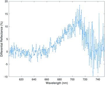
We organize the results into four different subsections. The first subsection shows the advantage of supervised dimension reduction over PCA even when there is limited number of data points; the second subsection shows the efficacy of supervised dimension reduction on separating interclass vapors; the third subsection shows the efficacy of supervised dimension reduction on separating the vapors using data from two different experimental setups; lastly, we used the K-nearest neighbor classification algorithm to classify the vapors after dimension reduction.

The raw input data consist of differential reflectance measured over a large number of wavelengths. An example of a raw input data point is shown in Fig. 1. We used a combination of an in-house python code and the Scikit-learn machine learning library¹⁷ to perform the dimension reduction and classification of the results.

Fig. 1 An example of the differential reflectance spectra for the DCM vapor.

3.1 Experimental data with small number of data points

The first dataset is taken from Kittle et al.² The reflectance data was generated by monitoring light reflected from the natural photonic crystal found in the wings of a Morpho didius butterfly upon exposure to vapor. The vapors used in this experiment were 1,5-dicholoropentane (DCP), dimethyl methylphosphonate (DMMP), ethanol (EtOH), methanol (MeOH) and water. The vapors were tested at 15%, 25% and 50% of the saturation concentration of each vapor, generating significantly different vapor concentrations. Generally, the vapor concentrations of the CWA simulants were much lower than the other more common vapors. Due to the time-consuming nature of the experiments, there were only 15 data points available: three data points for each vapor. Each input data point consists of reflectance measurements at 1008 different wavelengths. We applied all five dimension reduction methods to reduce the input data dimension from 1008 to two dimensions. In order to apply the supervised dimension reduction, we split the dataset into training and testing datasets. Two-thirds of the data points were used for training and one-third of the data points were used for testing and evaluation of the dimension reduction.

The results for all five dimension reduction methods are shown in Fig. 2. The ovals in the figure are drawn schematically. They mark the areas occupied by data points from different vapors. As shown in Fig. 2a, d, and e, the vapor separations using PLS and SPCA are comparable to the separations in PCA. The principal components selected by the methods LDA (Fig. 2b) and LSR-PCA (Fig. 2c) yielded more smaller and well-separated clusters compared to PCA, improving the selectivity of the analyzed data.

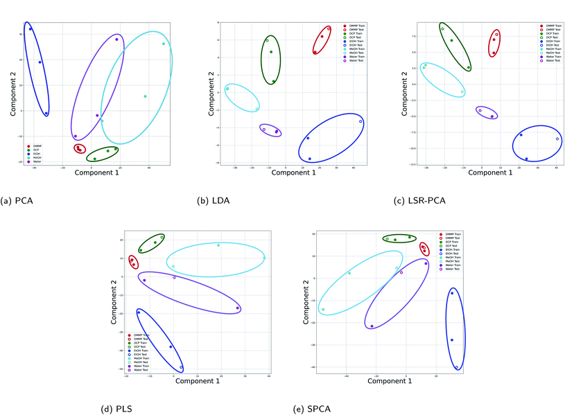Fig. 2 Projection onto two principal components for all five dimension reduction methods for the Morpho didius butterfly wing experimental data: (a) PCA; (b) LDA; (c) LSR-PCA; (d) PLS; (e) SPCA.

3.2 Simulated optical vapor reflectance data

In order to provide the supervised dimension reduction methods with a large dataset, we used a dataset that was computationally generated using the DiffractMod Software from Kittle et al.² The vapors included in this dataset are also DCP, DMMP, EtOH, MeOH and water. The dataset consists of reflectance data at 15%, 25% and 50% of the saturation concentration for each vapor. The computational model studied the reflectance of the vapor at 4501 different wavelengths. This dataset contained 60 data points. For the supervised dimension reduction methods, 80% of the data points were used training and 20% of the data points were used for testing and evaluation of the dimension reduction.

Fig. 3 shows how the five dimension reductions separated the vapors when projected onto two principal components. We see that all five methods performed well at intraclass separation: the CWA simulant vapors DCM and DMMP were clearly separated from the more common vapors EtOH, MeOH and water. Note that the CWA vapors have higher reflectance index compared to the other vapors as shown in Table 1. However, LDA and LSR-PCA provided better interclass separation within the two classes. Fig. 3b and c both show clear separation between DCM and DMMP, while PCA in Fig. 3a had a significantly more overlap between the CWA vapors.

Fig. 3 Projection onto two principal components for all five dimension reduction methods for the simulated Morpho didius butterfly wing data: (a) PCA; (b) LDA; (c) LSR-PCA; (d) PLS; (e) SPCA.

Table 1 Physical properties of the vapors

Gas	Refractive Index
DCM	1.424
DMMP	1.414
DCP	1.457
EtOH	1.361
MeOH	1.328
Water	1.333

---

3.3 Experimental data from different filters

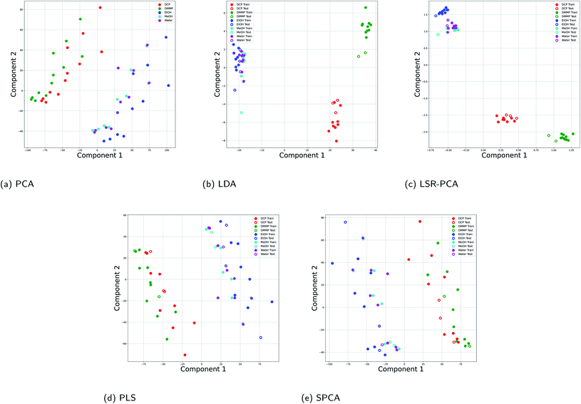
It is common in vapor sensing to use different sensors with partial selectivity, known as multi-sensor arrays. In this dataset, we combined optical vapor data using two rugate filter substrates: the first substrate is coated with an oxidized surface and the other one is coated with a carbonized surface. The experimental data was taken from Kittle et al.⁴ The experiments used five different vapors, dichloromethane (DCM), DCP, EtOH, MeOH and water at 2%, 5%, 10%, 20% and 30% of the saturation concentration. There are a total of 50 data points. Each data point consists of differential reflectance at 438 wavelengths. For the supervised dimension reduction methods, 80% of the data points were used training and 20% of the data points were used for testing and evaluation of the dimension reduction.

Fig. 4 shows the results using all five dimension reduction methods. The results from the two different filters are denoted by different markers: circle markers for the oxidized surface and square markers for the carbonized surface. Fig. 4a shows that the principal components selected by PCA focused on separating the two experimental setup. This is shown by the two distinct lines of circle data points and square markers. The variance of in the input data matrix X caused by the different experimental setup dominates the selection of the principal components. A similar behavior is seen in SPCA and PLS in Fig. 4e and d. However, LDA and LSR-PCA selected principal components that focus on distinguishing the different vapors as shown in Fig. 4b and c. LDA and LSR-PCA performed well on multi-sensor reflectance data because the optimization principles (Section 2.2 and 2.3) for these two methods emphasize the separation between different vapors.

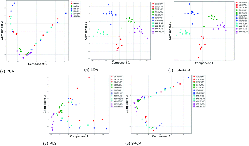Fig. 4 Projection onto two principal components for all five dimension reduction methods for the experimental results using two rugate filers: (a) PCA; (b) LDA; (c) LSR-PCA; (d) PLS; (e) SPCA.

3.4 Classification after dimension reduction

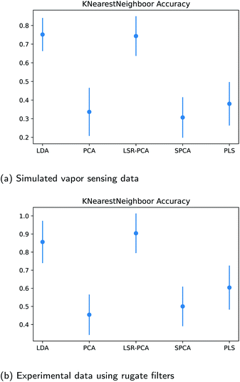
Next, we want to assess how well a classification method can identify the different vapors after reducing the raw input data to two dimensions. The K-nearest neighbor method was applied to the dimension-reduced input data matrix for the datasets in Section 3.2 and 3.3. The number of neighbors K was picked using the five-fold cross-validation technique for each calculation. In order to identify the effects due to different train-test splits of the data, we examined the K-nearest neighbor classification accuracy over 50 different random train-test splits of the reflectance data. The average and the first standard deviation of the classification accuracy are shown in Fig. 5a and b. As expected, the classification accuracy after applying LDA and LSR-PCA far exceeds the accuracy using PCA, SPCA and PLS.

Fig. 5 Classification accuracy using K-nearest neighbor using 50 different randomly generated train-test splits for each dimension reduction method: (a) simulated vapor sensing data; (b) experimental data using rugate filters.

3.5 Effects of training data size

Supervised dimension reduction methods require a fraction of the existing data for training. For some applications, training data can be costly to obtain. In this section, we study the effect of training data sizes for two of the supervised dimension reduction methods: LDA and LSR-PCA. The resulting plots are known as the learning curve for the supervised dimension methods. For each of the two methods, we assessed the prediction accuracy on the testing data using 20%, 40%, 60% and 80% of the data for training. The raw training data was reduced to two dimensions. The prediction accuracy on the testing data is averaged over 50 different random train-test splits. K-nearest neighbors method was used to classify the vapors. The parameter K in the K-nearest neighbor method was selected using five-fold cross-validation technique. We performed this study on the simulated vapor sensing data and the experimental data using rugate filters. The learning curve for LDA and LSR-PCA for the simulated vapor sensing data is shown in Fig. 6. The slope of the learning curve indicates that more training data would be able to improve the accuracy of the models. The learning curves for LDA and LSR-PCA for the experimental data from different filters are shown in Fig. 7. The slope of the learning curve has plateaued; this indicates that additional training data will not provide much benefit to improving the model.

Fig. 6 Learning curve for the simulated vapor data using LDA and LSR-PCA: (a) LDA; (b) LSR-PCA.

Fig. 7 Learning curve for the experimental vapor data using LDA and LSR-PCA: (a) LDA; (b) LSR-PCA.

4 Conclusions

In this paper, we have compared five supervised dimension reduction methods with the PCA method on optical vapor sensing data. We showed through using both experimental and computational data that two of the supervised dimension reduction methods, LDA and LSR-PCA outperformed all remaining methods in identifying the different vapors. Specifically, the supervision algorithms in LDA and LSR-PCA were able sift out the unimportant variances in the input data matrix such as intraclass differences and different experimental setup. We showed that LDA and LSR-PCA greatly enhanced the ability of machine learning methods to classify optical vapor sensing data.

Data availability

The data and code that support the findings of this study are openly available in the Github repository at https://github.com/meierms1/Supervised-Dimension-Reduction-For-Optical-Vapor-Sensing.

Author contributions

Maycon Meier: formal analysis, investigation, methodology, software, validation, visualization, writing-original draft; Josh D. Kittle: data curation, resources, supervision, validation, writing-review & editing; Xin C Yee: conceptualization, funding acquisition, data curation, project administration, resources, supervision, validation, and writing-review & editing.

Conflicts of interest

There are no conflicts to declare.

Acknowledgements

The authors acknowledge the University of Colorado Colorado Springs for providing funding for Maycon Meier for his PhD studies.

References

1. T. Jiang, Z. Peng, W. Wu, T. Shi and G. Liao, Sens. Actuators, A, 2014, 213, 63–69.
2. J. D. Kittle, B. P. Fisher, A. J. Esparza, A. M. Morey and S. T. Iacono, ACS Omega, 2017, 2, 8301–8307.
3. J. D. Kittle, B. P. Fisher, C. Kunselman, A. Morey and A. N. Abel, Sensors, 2019, 20(1), 157.
4. J. D. Kittle, J. S. Gofus, A. N. Abel and B. D. Evans, ACS Omega, 2020, 5, 19820–19826.
5. R. A. Potyrailo, H. Ghiradella, A. Vertiatchikh, K. Dovidenko, J. R. Cournoyer and E. Olson, Nat. Photonics, 2007, 1, 123–128.
6. R. Potyrailo and R. R. Naik, Annu. Rev. Mater. Res., 2013, 43, 307–334.
7. R. A. Potyrailo, R. K. Bonam, J. G. Hartley, T. A. Starkey, P. Vukusic, M. Vasudev, T. Bunning, R. R. Naik, Z. Tang and M. A. Palacios, et al., Nat. Commun., 2015, 6, 1–12.
8. R. A. Fisher, Ann. Hum. Genet., 1936, 7, 179–188.
9. H. Hotelling, J. Educ. Psychol., 1933, 24, 417.
10. H. Wold, J. Appl. Probab., 1975, 12, 117–142.
11. K. Fukumizu, F. R. Bach and M. I. Jordan, Ann. Stat., 2009, 37, 1871–1905.
12. E. Bair, T. Hastie, D. Paul and R. Tibshirani, J. Am. Stat. Assoc., 2006, 101, 119–137.
13. E. Barshan, A. Ghodsi, Z. Azimifar and M. Z. Jahromi, Pattern Recogn., 2011, 44, 1357–1371.
14. H. Pascual and X. Yee, Numerical Linear Algebra with Applications, 2020, p. e2411.
15. K. Pearson, On lines and planes of closest fit to systems of points in space, The London, Edinburgh, and Dublin Philosophical Magazine and Journal of Science, 1901, 2, 559–572.
16. A. Gretton, O. Bousquet, A. Smola and B. Schölkopf, International conference on algorithmic learning theory, 2005, pp. 63–77.
17. F. Pedregosa, G. Varoquaux, A. Gramfort, V. Michel, B. Thirion, O. Grisel, M. Blondel, P. Prettenhofer, R. Weiss, V. Dubourg, J. Vanderplas, A. Passos, D. Cournapeau, M. Brucher, M. Perrot and E. Duchesnay, J. Mach. Learn. Res., 2011, 12, 2825–2830.

---

Footnote

† Electronic supplementary information (ESI) available. See DOI: 10.1039/d1ra08774f

---