 Open Access Article
Polysaccharide determination and habitat classification for fresh Dendrobiums with hyperspectral imagery and modified RBFNN
Yuzhen Weiab,
Wenjun Huab,
Feiyue Wuc and
Yi He *d
*d
aSchool of Information Engineering, Huzhou University, Huzhou, Zhejiang, China
bZhejiang Province Key Laboratory of Smart Management & Application of Modern Agricultural Resources, Huzhou, Zhejiang, China
cSchool of Materials and Chemical Engineering, Chongqing University of Arts and Sciences, Chongqing, China
dState Key Laboratory of Subtropical Silviculture, Zhejiang A&F University, Lin'an, Hangzhou, China. E-mail: yihezf@163.com
First published on 5th January 2022
Abstract
This research aimed to study the visual and nondestructive detection of mannose (MN) and Dendrobium polysaccharides (DP) in Dendrobiums by using hyperspectral imaging technology. In order to determine the MN and DP concentrations nondestructively, we built radial basis function neural network (RBFNN) models based on NIR spectra (874–1734 nm) with a novel chemometric method to calculate the radial bases. And excellent results with the RP2 coefficients of 0.906 and 0.913 were obtained by the MN and DP detection models, respectively. In order to simplify the detection models based on full-range spectra, we designed an innovative genetic algorithm-successive projections algorithm (GA-SPA) strategy to extract the feature bands efficiently in two stages. Based on the feature bands selected by GA-SPA, we established the simplified detection models with the same high performance as those based on full-range spectra. By importing the feature bands of every pixel in the hyperspectral image into the simplified detection models, we successfully generated the distribution maps of MN and DP. Moreover, we also built an RBFNN classifier to categorize the habitats of Dendrobium. And the total classification accuracy reached 0.887. This research makes progress in Dendrobium quality evaluation and spectral detection technology.
1. Introduction
Dendrobium is called the ‘gold of herbs’ in China to illustrate its great value. It has been treated as a rare tonic with a long story, and many medical experiments have proven its powers in health and disease prevention.1,2 In the natural environment, Dendrobium is hard to harvest because it is rare and grows on cliff crevices. To satisfy the consumption requirement, people plant Dendrobiums by simulating the natural growth environment with modern cultivation techniques.3 But the quality of different Dendrobium products varies distinctly. The mannose (MN) and Dendrobium polysaccharides (DP) are most representative to assess the Dendrobium quality.4 However, the traditional method used to determine MN and DP concentrations is HPLC. It is low-efficiency, destructive, regent consuming, and laborious.5 A real-time and nondestructive detection method is urgently needed.Hyperspectral imaging technology takes advantage of spectral and spatial information simultaneously. It fulfills the requirement of nondestructive detection because the spectral information can express internal chemical characteristics.6 Furthermore, the concentration of the internal chemical compounds can be determined rapidly by importing the feature spectral information into the regression models constructed previously. So, the detection method with hyperspectral imaging technology also satisfies the real-time requirement. Beyond the above merits, the chemical distribution characteristics can be observed visually by hyperspectral imaging. As it is so capable, hyperspectral imaging technology has been widely applied in the quality detection of food,7 medicine,8 and agriculture.9 But no research on Dendrobium detection with hyperspectral imaging has been reported.
Throughout the processes of hyperspectral imaging technology, the core is to build precise and robust detection models. Up to now, there have been many classical modeling methods for employment, such as principal component regression (PCR), partial least squares regression (PLSR),10 backpropagation neural network (BPNN), and radial basis function neural network (RBFNN). Among these classical methods, RBFNN and BPNN have the stronger ability to mine the nonlinear relationship between the input and output variables.11,12 Both BPNN and RBFNN are qualified for the task of regression and classification simultaneously. And, RBFNN is more efficient in coefficients learning compared to BPNN.13 Although RBFNN is an efficient tool, it is hard to identify the radial basis in the application with great quantity samples because both sparsity and completeness of radial basis must be guaranteed.14 Besides the ingenious operation in model construction, the simplicity and representativeness of input variables also greatly affect modeling performance. Hence, it is necessary to select representative bands and eliminate the redundant information of spectra. Similar to the situation of modeling, many feature selection methods can be referenced. Some are intelligent swarm algorithms, such as genetic algorithm (GA)15 and artificial immune algorithm (AIA).16 And some are mathematical methods, such as successive projections algorithm (SPA)17 and uninformative variable elimination (UVE).18 The intelligent swarm algorithms and mathematical methods have different places they are good at. In the traditional operation way, different feature selection methods are adopted individually or combined ramblingly. It is not conducive to exploiting the comprehensive advantages of the two kinds of methods.
This research focuses on the visual detection of MN and DP and categorization in Dendrobiums. During the mission of feature selection and model establishment, novel schemes were designed to improve performance. In addition, the influence of habitat factors on MN and DP, and Dendrobium habitats classification were studied.
2. Materials and methods
2.1 Sample preparation and data acquisition
The Dendrobiums were collected from Anhui province (AH), Zhejiang province (ZJ), Guangxi province (GX), Yunnan province (YN), and Hunan province (HN) in April 2020. A total of 268 fresh samples were obtained. Before data acquisition, the leaves and roots of the Dendrobium samples were removed from the plants as the stem is the edible part.19 Subsequently, the hyperspectral images of the stems were captured. Then, the stems were destroyed to determine their MN and DP concentrations.A hyperspectral image acquisition system was used to capture the hyperspectral images. The system's illumination is provided by a linear light resource (Fiber-Lite DC 950, Dolan Jenner Industries Co., Ltd, USA). The system's hyperspectral camera (ImSpector V10E, SPECIM Spectral Imaging Oy Co., Ltd, Finland) worked in the range of 874–1734 nm, and the spectral resolution is 5 nm. The system captures hyperspectral images in a linear scanning mode, and the spatial resolution of each line is 320 pixels. During the hyperspectral image acquisition, the distance between the sample and the lens was set to 300 mm, the scanning speed was set to 17 mm s−1, and the exposure time was set to 3 ms. The reference values of the MN and DP concentrations were determined by a high-performance liquid chromatography (HPLC) instrument (LC-16P, Shimadzu Co., Ltd, Japan). The purity of MN and DP standards (China Pharmaceutical Group Co., Ltd, China) is greater than 99%. Before HPLC determination, the stem flesh was ground fully.
At last, 268 hyperspectral images and 268 × 2 (chemical indexes) concentration values were acquired for analysis.
2.2 Model establishment and evaluation
PLSR and RBFNN were adopted to establish detection models. PLSR fits the relationship between the spectra and the concentration values by minimizing the square sum of fitting errors. Specifically, multiple regression analysis, principal component analysis, and correlation analysis are executed in the PLSR model establishing.20 After principal component analysis and correlation analysis, the principal components with low collinearity and high representativeness were figured out by comprehensively taking the spectral information and concentration values into consideration. The multiple regression analysis of PLSR works on calculating the mapping coefficients from principal components to concentration values. However, RBFNN constructs the relationship between the spectra and the concentration values based on radial basis functions. The key parameters of the radial basis functions are function center C, function width σ, and the number of the centers N. The parameters C and σ shape the function with the formula ∅(X) = exp(−‖X − C2‖/σ), X is the input variable. All the radial basis functions synergistically determine the performance of RBFNN. The parameter σ is generally determined by the location of the function centers with the formula σ = d/2N, d is the distance between different centers. According to the above description and formulas, it can be found that the parameters C and N are the most important. And some classical methods, such as K-means clustering, random selection, and orthogonal least squares, were proposed to get the function center C. For K-means clustering, it is hard to set the number of clustering centers properly.21 For random selection, it is short of guidance. For orthogonal least squares, the number of function centers is set without reference either.22 In an objective opinion, the function centers should be identified according to the distribution characteristics, and the distribution of the centers should be measured by the distance between the spectra of all samples.23 Therefore, the Euclidean distances are calculated between all samples in this research, and a distance matrix is generated first. Based on the distance matrix, the total distance to other samples is calculated for each sample. Then, all the samples are sorted according to their total distances. In light of the samples that clustering together in the vector space may have similar total distances and adjacent ranking points, the similarity of every two adjacent samples in the sorted sequence is calculated with the cosine formula, so a corresponding similarity sequence is generated. The samples with short total distance and sharply changed similarity are selected in turn to form the bases. Meanwhile, the modeling performance of RBFNN is evaluated continuously with the increase of centers, and the optimal number of function centers is identified according to the performance evaluation. The modified RBFNN with the above strategy can be applied to regression and classification tasks, so the classifier of Dendrobium habitats is also established by the RBFNN.During regression analysis, RMSE, R2, RPD are adopted to evaluate the modeling performance. The RMSEC and RC2 are used to describe the model stability, while the RMSEP, RP2, and RPD are used to describe the model's predictive performance. For RMSE, the smaller, the better. For R2, the closer to 1, the better. For RPD, the bigger, the better. During classification analysis, the confusion matrix was adopted to evaluate the performance of classification models.
2.3 Feature bands selection
GA was proposed in the 1970s, and it has been applied in feature band selection of spectra for a long time. In GA, the spectrum of each sample is treated as a chromosome, and each band in the spectrum is treated as a gene.24 Some chromosomes coded in binary form are selected to construct the initial population. The RBFNN model is introduced as the fitness function to evaluate the chromosomes of the initial population. According to the evaluation results, the worst individuals are eliminated. The rest individuals exchange their gene sequences for renewing the population. In order to increase the genetic diversity, the mutation is performed on some genes after chromosomal crossover. Then, the new population after mutation is re-evaluated to select suitable individuals. The above operations are circularly executed until the population is satisfied or the circular times run out. As each gene corresponds to a band, the genes in the final population are counted to figure out the bands' importance. According to the bands' importance, the feature bands are finally identified.SPA is also a typical method to select feature bands, but it is quite different from the GA. It begins by identifying an initial feature band randomly, then projections from the rest bands to this initial feature band are calculated.25 The band with the largest projection value is chosen to join the feature bands group. The projection will be circularly calculated until enough feature bands are selected.
The GA and SPA play different roles in the feature bands selection. GA is good at identifying the feature bands explicable in chemical groups. But, the incident of abundance often occurs as the multiple adjacent bands may be assigned to the same function group. SPA has an inherent talent to eliminate the adjacency of feature bands as the projection distance between the adjacent bands is short. But, it is sensitive to the initial feature band.
3. Results and discussion
3.1 Overview on spectra and chemical concentrations
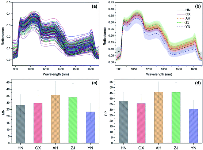
The spectra of all samples are basically consistent in waveform (Fig. 1a). Namely, all the spectra own the same peaks and troughs. The NIR spectra are the overlap curves of the sum of overtones and combination bands from vibrational bands. Therefore, the similar NIR curves reflect that the chemical compositions of all the samples are similar to each other.26 The spectra of different samples show gradients at reflectance. It means that the concentrations of the contents inside the samples are different. The average spectra from different habitats (Fig. 1b) exhibit different features at the spectral reflectance. It illustrates that there are differences in concentrations of the functional contents between different habitats. Besides, the average spectra from different habitats are not equally spaced. In other words, there are obvious differences in the spectral waveforms between different habitats. This will contribute to classifying the habitats of the Dendrobiums. The statistics on MN (Fig. 1c) and DP (Fig. 1d) testify to the inference from Fig. 1b. The average chemical concentrations of different habitats are obviously different. In terms of MN concentration, the habitats are sorted as AH, ZJ, GX, HN, YN in descending order. In terms of DP concentration, the habitats are sorted as AH, ZJ, HN, GX, YN in descending order. As a whole, the Dendrobiums from AH are the best at both MN and DP concentrations. In contrast, the Dendrobiums from YN are not so satisfied. According to the above analysis, it is necessary to determine the concentration of the functional contents and classify the category for Dendrobium, and the spectral information provides the probability to accomplish the task.3.2 Modeling analysis based on full-range spectra
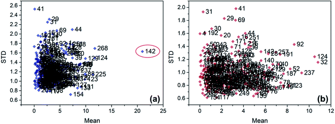
The improper operation, instrument fault, or wrong record will cause outliers. And the outliers have a negative effect on the model establishment. So, outliers should be detected and eliminated first. The common Monte Carlo sampling algorithm27 was adopted to detect the outliers. The number of iterations was set to 20![[thin space (1/6-em)]](https://www.rsc.org/images/entities/char_2009.gif) 000 in the execution of the algorithm. After all the iterations ran out, the mean and standard deviation (STD) of residuals were calculated for every sample. The sample with unnormal mean and STD was marked as the potential outlier (Fig. 2). If the model performance improves by eliminating the marked sample, the sample will be identified as the true outlier. Before outlier detection, we numbered every sample to find out the outliers conveniently. By testing, the 142nd sample was left out in the regression model establishment of MN. Then the remained samples were divided into calibration set and prediction set at a ratio of 2
000 in the execution of the algorithm. After all the iterations ran out, the mean and standard deviation (STD) of residuals were calculated for every sample. The sample with unnormal mean and STD was marked as the potential outlier (Fig. 2). If the model performance improves by eliminating the marked sample, the sample will be identified as the true outlier. Before outlier detection, we numbered every sample to find out the outliers conveniently. By testing, the 142nd sample was left out in the regression model establishment of MN. Then the remained samples were divided into calibration set and prediction set at a ratio of 2![[thin space (1/6-em)]](https://www.rsc.org/images/entities/char_2009.gif) :
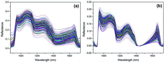
:![[thin space (1/6-em)]](https://www.rsc.org/images/entities/char_2009.gif) 1 according to the K–S algorithm.28 The PLSR models were first built by the calibration set and tested by the prediction set to testify the feasibility of spectral detection on Dendrobiums. For both MN and DP, the RP2 values of PLSR models are greater than 0.84 (Table 1). That means there's a strong relationship between the spectra and the concentrations. With the consideration that random noise and baseline drift is common in spectra acquisition, wavelet transform smooth29 and first derivative differential30 were carried out on the spectra, respectively (Fig. 3). However, the modeling performance has not improved after the pretreatments. Therefore, there is no apparent interference in the spectra acquisition, and further analysis is performed based on the raw spectra and RBFNN modeling method. Compared to PLSR models, the RBFNN models are better at stability and predictability. And, the better modeling performance of RBFNN mainly results from its powerful ability to dig out the nonlinear relationship between the spectra and the two chemical concentrations. Moreover, the RBFNN-modified models show evidently better performance than RBFNN-normal, so the scheme about function centers identification proposed in Section 2.2 is effective.
1 according to the K–S algorithm.28 The PLSR models were first built by the calibration set and tested by the prediction set to testify the feasibility of spectral detection on Dendrobiums. For both MN and DP, the RP2 values of PLSR models are greater than 0.84 (Table 1). That means there's a strong relationship between the spectra and the concentrations. With the consideration that random noise and baseline drift is common in spectra acquisition, wavelet transform smooth29 and first derivative differential30 were carried out on the spectra, respectively (Fig. 3). However, the modeling performance has not improved after the pretreatments. Therefore, there is no apparent interference in the spectra acquisition, and further analysis is performed based on the raw spectra and RBFNN modeling method. Compared to PLSR models, the RBFNN models are better at stability and predictability. And, the better modeling performance of RBFNN mainly results from its powerful ability to dig out the nonlinear relationship between the spectra and the two chemical concentrations. Moreover, the RBFNN-modified models show evidently better performance than RBFNN-normal, so the scheme about function centers identification proposed in Section 2.2 is effective.
| Modeling method | Chemical index | RMSEC | RC2 | RMSEP | RP2 | RPD |
|---|---|---|---|---|---|---|
| PLSR | MN | 3.815 | 0.851 | 3.870 | 0.849 | 2.576 |
| DP | 3.299 | 0.902 | 3.623 | 0.878 | 2.863 | |
| WT-PLSR | MN | 3.534 | 0.872 | 3.850 | 0.850 | 2.589 |
| DP | 3.355 | 0.898 | 3.708 | 0.872 | 2.797 | |
| FD-PLSR | MN | 3.750 | 0.854 | 4.367 | 0.808 | 2.284 |
| DP | 3.473 | 0.888 | 4.097 | 0.843 | 2.527 | |
| RBFNN-normal | MN | 3.511 | 0.874 | 3.631 | 0.867 | 2.747 |
| DP | 3.259 | 0.904 | 3.605 | 0.879 | 2.877 | |
| RBFNN-modified | MN | 2.751 | 0.921 | 3.158 | 0.906 | 3.278 |
| DP | 2.553 | 0.939 | 2.934 | 0.913 | 3.399 |
3.3 Modeling analysis based on feature bands and hyperspectral imaging
GA was first carried out on the raw spectra to select the feature bands of MN and DP. The initial population was set to 50, and each chromosome was encoded in binary mode. The length of the binary string is equal to the number of spectral bands. In the binary string, ‘0’ denotes the band at the corresponding position is not employed and ‘1’ denotes the band is employed. The crossover probability was set to 0.6, and a two-point crossover operator was adopted. The mutation rate was set to 0.01 to maintain the population diversity. Besides, the individual with the best performance was retained to the next generation directly by using external memory with elitism strategy. After 10![[thin space (1/6-em)]](https://www.rsc.org/images/entities/char_2009.gif) 000 iterations, the feature bands of MN and DP are distributed as Fig. 4a and b. For both MN and DP, the phenomenon of feature bands adjacency can be observed. This principally results from that the feature bands selected by GA are evaluated by the fitness function, and the adjacent bands often have close fitness values. In fact, the deeper reason lies in the assignment of chemical groups. The vibration of one function group corresponds to multiple consecutive bands, but only a few of the bands are most representative. Through refining the feature bands by SPA, the feature bands number of MN decreased from 50 (Fig. 4a) to 9 (Fig. 4c), and the feature bands number of DP decreased from 57 (Fig. 4b) to 14 (Fig. 4d). Compared with the RBFNN-modified modeling results based on full-range spectra (Table 1), the RBFNN-modified modeling results based on feature bands (Table 2) remain stable. For MN, the modeling performance improved slightly. While, for DP, the modeling performance decreased slightly. But due to the input variables' number decreasing greatly, the work efficiency of the model was deeply improved.
000 iterations, the feature bands of MN and DP are distributed as Fig. 4a and b. For both MN and DP, the phenomenon of feature bands adjacency can be observed. This principally results from that the feature bands selected by GA are evaluated by the fitness function, and the adjacent bands often have close fitness values. In fact, the deeper reason lies in the assignment of chemical groups. The vibration of one function group corresponds to multiple consecutive bands, but only a few of the bands are most representative. Through refining the feature bands by SPA, the feature bands number of MN decreased from 50 (Fig. 4a) to 9 (Fig. 4c), and the feature bands number of DP decreased from 57 (Fig. 4b) to 14 (Fig. 4d). Compared with the RBFNN-modified modeling results based on full-range spectra (Table 1), the RBFNN-modified modeling results based on feature bands (Table 2) remain stable. For MN, the modeling performance improved slightly. While, for DP, the modeling performance decreased slightly. But due to the input variables' number decreasing greatly, the work efficiency of the model was deeply improved.
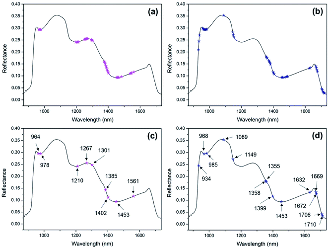 | ||
| Fig. 4 Feature bands of MN (a) and DP (b) selected by GA, feature bands of MN (c) and DP (d) selected by SPA after GA. | ||
| Feature bands | Chemical index | RMSEC | RC2 | RMSEP | RP2 | RPD |
|---|---|---|---|---|---|---|
| GA | MN | 2.670 | 0.926 | 2.902 | 0.915 | 3.437 |
| DP | 2.492 | 0.942 | 3.123 | 0.909 | 3.316 | |
| GA-SPA | MN | 2.738 | 0.922 | 3.014 | 0.908 | 3.309 |
| DP | 2.645 | 0.935 | 3.082 | 0.911 | 3.359 |
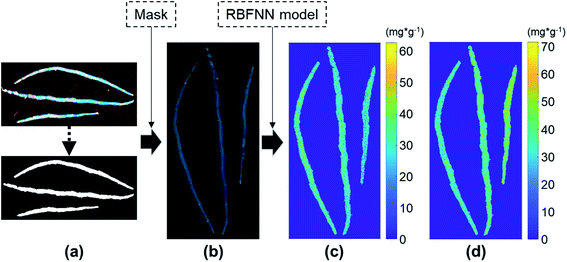
In the interest of obtaining the high-quality distribution maps of MN and DP concentrations, the raw hyperspectral image was masked with its binary image (Fig. 5a) first to remove the background. After background segmentation, the average spectrum of each single-connected region (Fig. 5b) was calculated to compress the tremendous fluctuation of the spectra belonging to different pixels. Then the GA-SPA feature bands of the adjusted spectra were input into the corresponding RBFNN model. At last, the distribution maps of MN (Fig. 5c) and DP (Fig. 5d) concentrations were generated. The difference in MN and DP concentrations between different Dendrobiums can be observed clearly. Besides, differences in different parts of the same individual are also exhibited.
3.4 Habitats classification analysis
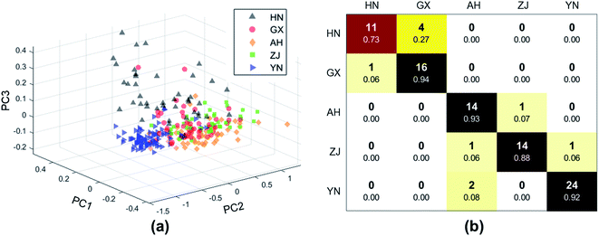
PCA was first performed to evaluate the feasibility of habitats classification. The first three PCs were employed to construct a 3-D scatter plot (Fig. 6a). It can be found that the distribution of samples from HN is rather dispersed in the space. For the rest four habitats, the samples cluster together. Even though the 3-D space was rotated at different angles, it is hard to divide the samples from different habitats in vision. Therefore, more PCs need to be employed to build the classifier. Before the classifier establishment, the samples were divided into calibration set and prediction set at a ratio of 2![[thin space (1/6-em)]](https://www.rsc.org/images/entities/char_2009.gif) :
:![[thin space (1/6-em)]](https://www.rsc.org/images/entities/char_2009.gif) 1 for each habitat. The calibration set was used to train the classifier, and the prediction set was used to test the classifier. RBFNN method was adopted to build the classifier. But unlike the regression task, the centers of the RBFNN used for classification consisted from the PCs of the spectra. By increasing the PCs one by one, the optimal PCs number is identified as 12. Finally, the total classification accuracy of the calibration set got 0.966, and the total classification accuracy of the prediction set got 0.887. The confusion matrix of the prediction set is shown in Fig. 6b. The HN and GX are easily confused with each other. Four HN samples were incorrectly classified as GX, and one GX sample was wrongly classified as HN. There is misclassification between AH and ZJ. These two cases can be explained by the statistics of MN and DP concentrations (Fig. 1c and d). The HN and GX are close at the concentrations, and AN and ZJ are close. As exceptions, one ZJ sample was misclassified as YN, and two YN samples were misclassified as AH. But, taken as a whole, it is feasible to classify the habitats of Dendrobiums based on RBFNN and spectral information. On the whole, the classification accuracy is not so excellent. It mainly results from that the habitat factor actually contains many sub-factors. And, each sub-factor, such as irrigation, fertilization, or soil condition, may vary highly. So, plant conditions need to be studied precisely to improve the classification accuracy.
1 for each habitat. The calibration set was used to train the classifier, and the prediction set was used to test the classifier. RBFNN method was adopted to build the classifier. But unlike the regression task, the centers of the RBFNN used for classification consisted from the PCs of the spectra. By increasing the PCs one by one, the optimal PCs number is identified as 12. Finally, the total classification accuracy of the calibration set got 0.966, and the total classification accuracy of the prediction set got 0.887. The confusion matrix of the prediction set is shown in Fig. 6b. The HN and GX are easily confused with each other. Four HN samples were incorrectly classified as GX, and one GX sample was wrongly classified as HN. There is misclassification between AH and ZJ. These two cases can be explained by the statistics of MN and DP concentrations (Fig. 1c and d). The HN and GX are close at the concentrations, and AN and ZJ are close. As exceptions, one ZJ sample was misclassified as YN, and two YN samples were misclassified as AH. But, taken as a whole, it is feasible to classify the habitats of Dendrobiums based on RBFNN and spectral information. On the whole, the classification accuracy is not so excellent. It mainly results from that the habitat factor actually contains many sub-factors. And, each sub-factor, such as irrigation, fertilization, or soil condition, may vary highly. So, plant conditions need to be studied precisely to improve the classification accuracy.
4. Conclusion
This research provides a complete scheme to determine the mannose and Dendrobium polysaccharides in Dendrobiums visually and nondestructively. The scheme will make significance to optimize the postharvest pretreatment, like processing, storage, and transportation of Dendrobiums. In the nondestructive detection scheme, some specific issues of chemometrics were studied. For the Dendrobiums with various factors, the matrix is quite different at chemical composition, especially the concentration of the main components. As the spectra can reflect the internal chemical features of plant, the Dendrobiums will exhibit individual spectral characteristics. That will bias the determination of the mannose and Dendrobium polysaccharides. Therefore, we designed a creative radial bases identification method for RBFNN to build the accurate mapping relationship between the spectra and the polysaccharide components. Moreover, we developed a novel strategy that used GA and SPA comprehensively to select the feature bands efficiently, and the model was greatly simplified, but the modeling performance still keeps stable. These will enrich the theory in RBFNN construction and feature bands selection. In addition, the habitats classification of Dendrobiums was also investigated. As the habitats have a strong connection to the products' quality and brand protection, the investigation of habitats classification will make assistance in standardizing the market of Dendrobiums.Although some creative work has been done, there are many other issues need to be researched to perfect the scheme and promote the practical application. First, we didn't set an experiment to explore the upper and lower bounds of detection range and the minimum variance of polysaccharide components which can be captured by the detection model. But, in some situations, such as drug development which needs to control the concentration of MNs and DPs precisely, it is important to clarify the sensitivity of the method proposed in this research. Second, we didn't discuss the interference from detection environment and sample discrepancy. In the real production, the detection environment is complicate and the categories of Dendrobiums are far more than three. We need to optimize the scheme to reduce the environment interference and improve the model transferability on different categories.
Author contributions
Conceptualization, Yuzhen Wei and Yi He; methodology, Feiyue Wu; software, Wenjun Hu; validation, Yuzhen Wei and Feiyue Wu; formal analysis, Yuzhen Wei; investigation, Feiyue Wu; resources, Wenjun Hu; data curation, Yuzhen Wei and Yi He; writing-original draft preparation, Yuzhen Wei; visualization, Yuzhen Wei; supervision, Yi He; project administration, Yuzhen Wei and Wenjun Hu; funding acquisition, Yi He and Wenjun Hu. All authors have read and agreed to the published version of the manuscript.Conflicts of interest
There are no conflicts of interest to declare.Acknowledgements
This work was supported by the National Natural Science Foundation of China (31801273, 61772198), the Department of Science and Technology of Ningbo (DSTNB, Project No. 2019C10008).References
- T. B. Ng, et al., Review of research on Dendrobium, a prized folk medicine, Appl. Microbiol. Biotechnol., 2012, 93(5), 1795–1803 CrossRef CAS PubMed.
- Y. Y. Cao, et al., Dendrobium candidum aqueous extract attenuates isoproterenol-induced cardiac hypertrophy through the ERK signalling pathway, Pharm. Biol., 2020, 58(1), 176–183 CrossRef CAS PubMed.
- J. Cheng, et al., An assessment of the Chinese medicinal Dendrobium industry: supply, demand and sustainability, J. Ethnopharmacol., 2019, 229, 81–88 CrossRef PubMed.
- X. M. Chen, et al., Discrimination of the rare medicinal plant Dendrobium officinale based on naringenin, bibenzyl, and polysaccharides, Sci. China: Life Sci., 2012, 55(12), 1092–1099 CrossRef CAS PubMed.
- Z. Yuan, G. Cong and J. Zhang, Effects of exogenous salicylic acid on polysaccharides production of Dendrobium officinale, S. Afr. J. Bot., 2014, 95, 78–84 CrossRef CAS.
- Y. Z. Wei, Y. He and X. L. Li, Tea moisture content detection with multispectral and depth images, Comput. Electron. Agr., 2021, 183, 106082 CrossRef.
- M. Zhu, et al., Application of hyperspectral technology in detection of agricultural products and food: a review, Food Sci. Nutr., 2020, 8(10), 5206–5214 CrossRef PubMed.
- S. Wilczynski, et al., The use of hyperspectral imaging in the VNIR (400-1000 nm) and SWIR range (1000-2500 nm) for detecting counterfeit drugs with identical API composition, Talanta, 2016, 160, 1–8 CrossRef CAS PubMed.
- A. Baiano, Applications of hyperspectral imaging for quality assessment of liquid based and semi-liquid food products: a review, J. Food Eng., 2017, 214, 10–15 CrossRef CAS.
- G. Guven and H. Samkar, Examination of dimension reduction performances of PLSR and PCR techniques in data with multicollinearity, Iran. J. Sci. Technol., Trans. A: Sci., 2019, 43(3), 969–978 CrossRef.
- F. Douak, N. Benoudjit and F. Melgani, A two-stage regression approach for spectroscopic quantitative analysis, Chemom. Intell. Lab. Syst., 2011, 109(1), 34–41 CrossRef CAS.
- X. Y. Liu, et al., Comparison of prediction power of three multivariate calibrations for estimation of leaf anthocyanin content with visible spectroscopy in Prunus cerasifera, PeerJ, 2019, 7, e7997 CrossRef PubMed.
- G. Y. Chen, et al., Artificial neural network models for the prediction of CO2 solubility in aqueous amine solutions, Int. J. Greenhouse Gas Control, 2015, 39, 174–184 CrossRef CAS.
- F. Fernandez-Navarro, C. Hervas-Martinez and P. A. Gutierrez, Generalised Gaussian radial basis function neural networks, Soft Comput., 2013, 17(3), 519–533 CrossRef.
- A. Paul, et al., Band selection in hyperspectral imagery using spatial cluster mean and genetic algorithms, GIScience & Remote Sensing, 2015, 52(6), 643–659 Search PubMed.
- J. Feng, et al., Unsupervised feature selection based on maximum information and minimum redundancy for hyperspectral images, Pattern Recognit., 2016, 51, 295–309 CrossRef.
- S. F. Carreiro Soares, et al., A modification of the successive projections algorithm for spectral variable selection in the presence of unknown interferents, Anal. Chim. Acta, 2011, 689(1), 22–28 CrossRef PubMed.
- X. J. Chen, D. Wu and Y. He, An integration of modified uninformative variable elimination and wavelet packet transform for variable selection, Spectroscopy, 2011, 26(4), 42–47 Search PubMed.
- Z. M. Yu, et al., Influence of low temperature on physiology and bioactivity of postharvest Dendrobium officinale stems, Postharvest Biol. Technol., 2019, 148, 97–106 CrossRef CAS.
- I. S. Helland, et al., Model and estimators for partial least squares regression, J. Chemom., 2018, 32(9), e3044 CrossRef.
- R. Assaf, et al., Efficient classification algorithm and a new training mode for the adaptive radial basis function neural network equaliser, IET Communications, 2012, 6(2), 125–137 CrossRef.
- Y. Hu, et al., An eigenvector based center selection for fast training scheme of RBFNN, Inf. Sci., 2018, 428, 62–75 CrossRef.
- G. R. Chegini, et al., Prediction of process and product parameters in an orange juice spray dryer using artificial neural networks, J. Food Eng., 2008, 84(4), 534–543 CrossRef.
- R. J. Kowalski, C. J. Li and G. M. Ganjyal, Optimizing twin-screw food extrusion processing through regression modeling and genetic algorithms, J. Food Eng., 2018, 234, 50–56 CrossRef.
- Q. Dai, et al., Potential of visible/near-infrared hyperspectral imaging for rapid detection of freshness in unfrozen and frozen prawns, J. Food Eng., 2015, 149, 97–104 CrossRef.
- X. L. Chu, Molecular Spectroscopy Analytical Technology Combined with Chemometrics and Its Applications, Chemical Industry Press, 2011 Search PubMed.
- Y. Z. Wei, X. L. Li and Y. He, Generalisation of tea moisture content models based on VNIR spectra subjected to fractional differential treatment, Biosyst. Eng., 2020, 205, 174–186 CrossRef.
- M. F. Andrada, et al., Impact assessment of the rational selection of training and test sets on the predictive ability of QSAR models, SAR QSAR Environ. Res., 2017, 28(12), 1011–1023 CrossRef CAS PubMed.
- X. S. Wang, D. W. Qi and A. M. Huang, Study on denoising near infrared spectra of wood based on wavelet transform, Spectrosc. Spectral Anal., 2009, 29(8), 2059–2062 CAS.
- A. Q. Hu, et al., A correction method of baseline drift of discrete spectrum of NIR, Spectrosc. Spectral Anal., 2014, 34(10), 2606–2611 CAS.
| This journal is © The Royal Society of Chemistry 2022 |

