
 Open Access Article
 This Open Access Article is licensed under a Creative Commons Attribution-Non Commercial 3.0 Unported Licence
Quantifying nanoscale forces using machine learning in dynamic atomic force microscopy†
Abhilash
Chandrashekar
 *a,
Pierpaolo
Belardinelli
b,
Miguel A.
Bessa
c,
Urs
Staufer
a and
Farbod
Alijani
*a
*a,
Pierpaolo
Belardinelli
b,
Miguel A.
Bessa
c,
Urs
Staufer
a and
Farbod
Alijani
*a
aPrecision and Microsystems Engineering, TU Delft, Delft, The Netherlands. E-mail: a.chandrashekar@tudelft.nl; f.alijani@tudelft.nl
bDICEA, Polytechnic University of Marche, Ancona, Italy
cMaterials Science and Engineering, TU Delft, Delft, The Netherlands
First published on 5th April 2022
Abstract
Dynamic atomic force microscopy (AFM) is a key platform that enables topological and nanomechanical characterization of novel materials. This is achieved by linking the nanoscale forces that exist between the AFM tip and the sample to specific mathematical functions through modeling. However, the main challenge in dynamic AFM is to quantify these nanoscale forces without the use of complex models that are routinely used to explain the physics of tip–sample interaction. Here, we make use of machine learning and data science to characterize tip–sample forces purely from experimental data with sub-microsecond resolution. Our machine learning approach is first trained on standard AFM models and then showcased experimentally on a polymer blend of polystyrene (PS) and low density polyethylene (LDPE) sample. Using this algorithm we probe the complex physics of tip–sample contact in polymers, estimate elasticity, and provide insight into energy dissipation during contact. Our study opens a new route in dynamic AFM characterization where machine learning can be combined with experimental methodologies to probe transient processes involved in phase transformation as well as complex chemical and biological phenomena in real-time.
Introduction
Dynamic atomic force microscopy (AFM) has transitioned from a high resolution imaging technique to a versatile tool that provides spatially resolved maps of mechanical,1–4 chemical,5–7 and biological properties8–10 of samples. This transition is primarily fueled by the interest of the scientific community in precise quantification of materials at the nanoscale, which can be achieved by probing the tip–sample interaction force.11,12 However, dynamic AFM, in contrast to its name, does not directly measure the interaction force while imaging in any of its modalities. Instead, it uses different information channels like frequency, amplitude, and phase of the oscillating probe to reconstruct the interaction force indirectly.11–17Tip–sample reconstruction in dynamic AFM is essentially an inverse problem,18–20 where the measured deflection data is used to infer the underlying interaction physics and thus estimate parameters that are not directly observed. The reconstruction techniques in dynamic AFM are broadly categorized into two classes: analytical methods that rely on slow variations of amplitude and phase of the cantilever,13–15 and experimental techniques that depend on the spectral components generated due to the nonlinear nature of the tip–sample contact.11,12,17 Although versatile in discerning the tip–sample force, analytical methods can only obtain an averaged interaction force and not the instantaneous changes of it during the oscillations; a scenario that is of importance when probing biological and chemical processes.21–24 On the other hand, experimental techniques often follow a multi-step procedure to invert cantilever oscillations for obtaining the interaction force. These procedures either require measurement of the experimental transfer function12,17 or make use of special harmonic probes that are tailor-made to resolve the interaction force with high-resolution.11 Thus, despite the success of dynamic AFM in topography mapping and nanoscale imaging in its diverse modes of operation,25–27 a generic approach that allows direct access to the time-resolved surface forces, irrespective of the chosen probe-sample configuration is still missing.
Here, we develop a novel method for predicting the tip–sample interaction forces of dynamic AFM by making use of the recent advances in data science30,31 and machine learning32–36 that are well-suited for tackling inverse problems. In particular, we make use of sparse identification of nonlinear dynamical systems30,32–34,37 to distill the dynamics of AFM cantilever interacting with stiff and compliant samples. We train the algorithm on numerically generated data from several standard AFM models, and use that to discover physically interpretable models in experiments on a polymer blend of polystyrene (PS) and low-density polyethylene (LDPE). The obtained models are able to predict the time-resolved nanoscale forces between the AFM tip and polymers with sub-microsecond resolution. Additionally, our method can estimate the elasticity of different materials within the sample and also provide insight into hysteresis and energy dissipation during contact. Our machine learning technique goes beyond complex models that are often used for nano-characterization and has no inherent assumptions on the type of interactions, instead, it relies solely on the extracted temporal data from AFM measurements.
Results
Formulation
In order to obtain the tip–sample interaction force, we begin by finding the governing equations of AFM using a unified sparse identification framework known as sparse relaxed regularized regression.32,33,38 This approach aims at finding the equations of nonlinear dynamical systems of the form| ẋ(t) = f(x(t)), | (1) |
 is the state of the dynamical system at time t in the experimental time frame. Here, f is a nonlinear function that maps the dynamical state vectors to that of the experimental observables. In order to retrieve a minimal set of f, a library of linear and nonlinear candidate functions Θ(X) = [θ1(X)θ2(X)…θn(X)] is introduced such that
| f(x(t)) = Θ(X)Ξ, |
 | (2) |
In eqn (2), R(·) is the regularization term that promotes sparsity and minimizes over-fitting. In our study, we choose R(·) as the l0 norm of the auxiliary variable W. This variable is introduced here to enable relaxation and partial minimization in order to improve the conditioning of the problem and tackle the non-convexity of the optimization.33 In addition, λ and ν are hyper-parameters that control the strength of regularization and relaxation, respectively. Finally, in order to find physics-inspired models, we incorporate constraints derived from AFM experiments through matrices C and d (see Methods). In particular, these constraints make sure that during model discovery the stiffness k, quality factor Q, and external force Fc exerted on the cantilever match those from experiments.
Training
We begin by training the algorithm over numerically generated data sets from several standard AFM models. For the sake of clarity, we explain the training methodology on the data obtained from a Derjaguin–Muller–Toporov (DMT) model here.39 The training data includes both the transient and steady-state interactions typically observed during scanning operation in dynamic AFM as shown in Fig. 1.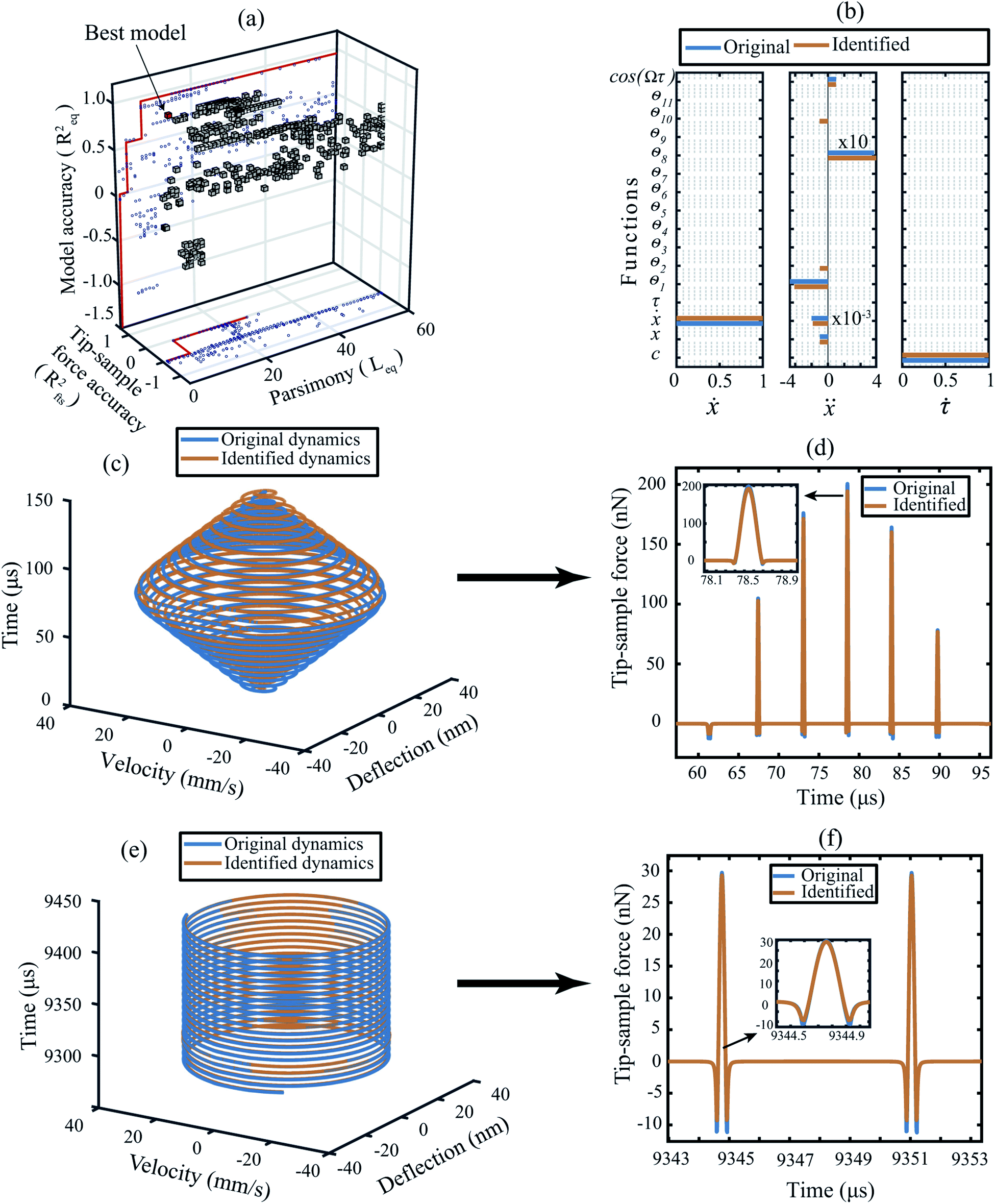 | ||
| Fig. 1 Training the algorithm on numerically generated data obtained for a cantilever with DMT force model described in ESI Section S1†.28,29 (a) 3D pareto frontier with parsimony, accuracy of the predicted model, and the tip–sample force as the selection parameters. The blue dots indicate the projection of the 3D cubes onto 2D planes. In the (x, z) plane the red line indicates the pareto optimal line between parsimony and the model accuracy; whereas, in the (x, y) plane it is the optimal line between the parsimony and the tip–sample force accuracy. The best model in this 3D space is highlighted by a red cube. (b) Coefficient matrix showing the influence of each library function on the governing equations. The blue color indicates the original value of the coefficients and the orange color indicates the coefficients as determined by the data-driven algorithm. The description of the functions are given in Table 1. (c and d) Transient dynamics prediction: comparison of the state vectors and the tip–sample force between the DMT simulation (blue) and the data-driven model (orange). (e and f) Steady-state response prediction: comparison of the state vectors and the tip–sample force between the DMT simulation (blue) and the data-driven model (orange). Additional details on selection of hyper-parameters and constraints on the optimization are provided in the Methods section. | ||
In our study, the library Θ(X) consists of constants, polynomials, and trigonometric terms of X. To predict the true physics of interaction, we also incorporate nonlinear functions in Θ(X) that are derived from consolidated AFM models (e.g., DMT,39 Johnson, Kendall and Roberts (JKR)40 and Lennard-Jones (LJ)50 as discussed in the ESI Section S1†).
In addition to the functions describing the tip–sample interactions, the library also includes bridging functions that mediate a smooth switch between the attractive and repulsive forces experienced by the tip's trajectory at the intermolecular distance (a0). Overall, we used 500 functions θi in the training phase of the analysis. To mimic experimental conditions, we also corrupted the numerically generated state vectors X with 1% Gaussian noise with zero mean. This signal is then de-noised and differentiated by using Savitzky–Golay algorithm41,42 to obtain the velocity, and acceleration vectors.
Before proceeding with the sparse identification, elimination of non-candidate functions from the library Θ(X) is necessary to improve the interpretability of the predicted models and avoid ill-conditioned matrices or large computational times.34 In order to achieve this, we augment the optimization problem defined in eqn (2) with constraints derived from experiments,43 the details of which are provided in the Methods section.
Finally, the de-noised data and the constraints are fed into the data-driven algorithm as part of a final routine in which the hyper parameters λ and ν are swept in a 2D space to obtain an approximate model capable of predicting the dynamics of the system. For each configuration of hyper-parameters, we perform 10 instance of rolling cross-validation with each instance running 250 iterations of an optimization routine to determine the optimum value of the coefficients. The optimization objective is defined such that the identification routine will find the best parsimonious model by penalizing the goodness of fit value based on the number of terms present in that particular model. In other words, the lengthier the equation of motion the more penalty the model is awarded. This not only promotes parsimony but also improves the general interpretability of the predicted model.
Numerical results
In order to identify the best model that can approximate the dynamics of the system, we build a three dimensional (3D) pareto diagram as shown in Fig. 1(a). The 3D Pareto frontier is calculated by plotting parsimony (the length of the identified equation of motion Leq) on the x-axis, the accuracy of state vector prediction on the z-axis (Req) and the accuracy of the tip–sample force on the y-axis (Rfts). The best model is readily identifiable by following the marked red line at the sharp drop in prediction accuracy (marked by the red cube). In Table 1 we list the candidate functions that represent the best model, and in Fig. 1(b) we compare the coefficients of this identified model (orange line) against the original DMT model (blue line) based on which the numerical data were generated. It can be seen that the identified coefficients are within 1% of their true values.| Function ID | θ 1 | θ 2 | θ 3 | θ 4 | θ 5 | θ 6 | θ 7 | θ 8 | θ 9 | θ 10 | θ 11 |
|---|---|---|---|---|---|---|---|---|---|---|---|
| Function definition | z −2 | z −3 |
δ
0.5
![[small delta, Greek, dot above]](https://www.rsc.org/images/entities/i_char_e14e.gif)
|
δ
2
|
z 0.5 ż | zż 2 | δ 2 | δ 2.5 | δ 1.5 | z −2 ∀z ≤ a0 | sin(Ωτ) |
We also note that the data-driven approach has led to two additional functions, namely θ2 and θ10 that were not present in the original model. This can be understood by comparing the total number of blue lines vs. orange lines in Fig. 1(b). Among the two, θ2 appears in the identified model purely due to the noise added to the state vectors. Whereas, θ10 acts as a bridging function to connect the non-smooth interaction forces namely, the non-contact van der Waals and the contact repulsive forces. We highlight that the DMT model inherently contains a bridging function in the form of adhesion force given by fadh = C3/a02 (see Section S1 of the ESI†).
To clarify this observation further, we compare the transient and steady-state response of the predicted model with the true dynamics in Fig. 1(c) and (e). We observe that the motion of the cantilever is well-replicated with an accuracy of 95% in a 3D phase space. The resulting 5% estimation error is due to the deviation of the identified coefficients from the true values which causes a small shift in the phase value between the original and the identified trajectories (for details, see ESI Section S1†).
Irrespective of this slight discrepancy, the ability of the selected model to unravel the corresponding tip–sample interaction force stands out in Fig. 1(d) and (f).
Fig. 1(d) shows the development of transient tip–sample interaction force when the cantilever encounters a step like feature during the scanning; whereas, Fig. 1(f) shows the steady-state tip–sample interaction force when the cantilever is imaging a uniform surface. In both cases, the blue and the orange colors represent the original and the identified force signals and the negative and positive force values indicate attractive and repulsive forces, respectively. The inset in both figures highlights the ability of the data-driven algorithm to identify specific features of interaction with sub-microsecond precision.
Finally, we remark that the algorithm has an accuracy of 99% in predicting the repulsive or contact interaction and 94% accuracy in predicting the attractive or non-contact interaction. These numbers drop down to approximately 82% near the interatomic distance where both contact and non-contact interactions co-exist. This is primarily due to the non-smooth nature of the contact and the lack of resolution in data points to approximate the behaviour of the system near the minima of the potential well.
Experiments
Based on the insights gained from the synthetic data-sets, we extend the formulation to experimental data and follow the methodology presented in Fig. 2. We begin by acquiring the raw deflection signal of an AFM cantilever directly from the photodetector using a Field Programmable Gated Array (FPGA) (see Methods). We estimate the tip–sample force for two sets of experiments using a silicon cantilever tapping on a two component polymer blend made of PS and LDPE. In the first experiment, we read-out the motion of the cantilever at a fixed distance from the sample, and in the second, we move the cantilever from a distance with zero-interaction to a point with maximum repulsive force similar to conventional dynamic spectroscopy measurements (see Fig. 2(b)). In both experiments, the acquired time signal is processed as described in the training procedure. Furthermore, we reduce the library of the candidate functions to a smaller subset of 40 functions. Next, we regress the AFM dynamics onto this library (see Fig. 2(c)) and estimate the instantaneous tip–sample force (see Fig. 2(d)).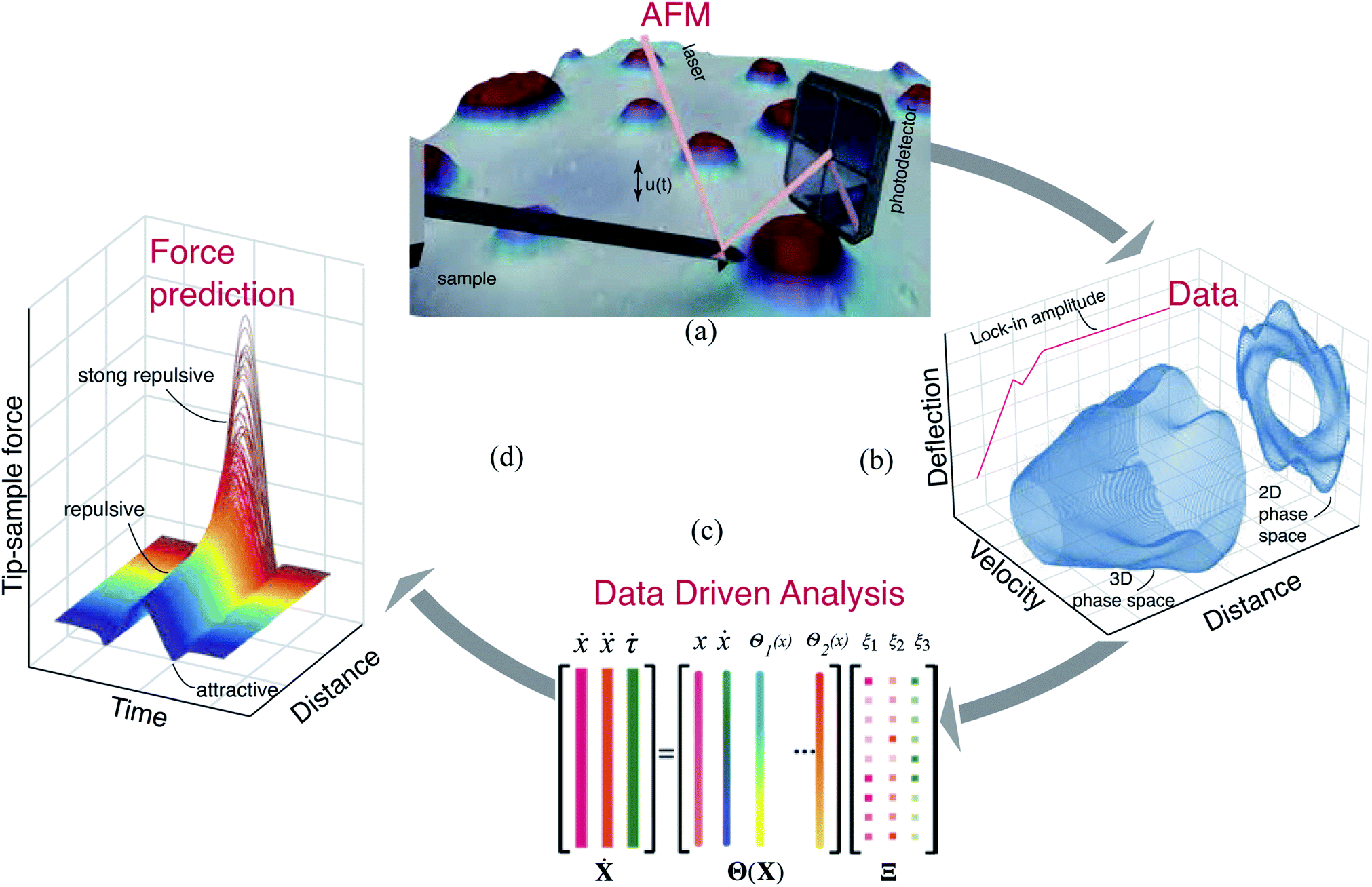 | ||
| Fig. 2 Schematic of the identification process. (a) Experimental data is obtained directly from the photodetector of the AFM. (b) The data is captured using an FPGA device and post-processed to create state vector channels. (c) The state vectors are used as inputs in the sparse identification algorithm to discover the governing model of the system. (d) The data-driven model is used to estimate the tip–sample interaction force. | ||
Fig. 3 shows the identification of the cantilever motion and the estimation of the interaction force when the probe is engaged with the PS polymer matrix at a fixed distance of 66 nm from the sample. It can be observed from the 3D phase space shown in Fig. 3(a) that our data-driven approach successfully captures the cantilever dynamics, and that the identified model follows the true experimental trajectory with an accuracy of 90%.
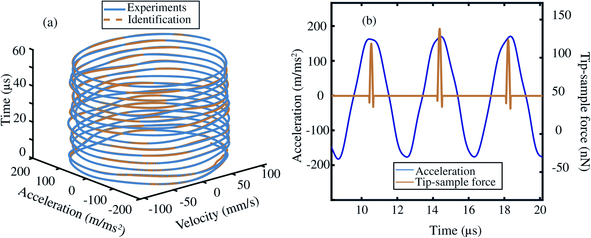 | ||
| Fig. 3 Data-driven identification for a silicon cantilever interacting with PS sample. The experimental deflection is obtained at a fixed tip–sample distance of 66 nm (a) identification of velocity and acceleration state vectors. The blue and orange curves represent the experimental and identified state space trajectories, respectively. (b) Estimation of the tip–sample force from data-driven model (orange) superimposed on the experimental acceleration signal (blue). | ||
In Fig. 3(b) we also show the estimated tip–sample force for several consecutive periods in the same experiment. It is interesting to note that the data-driven algorithm is capable to reconstruct the time–sample interaction from fast cantilever oscillations. A similar trend in behaviour for LDPE sample is also observed and showcased in the ESI Section S2.† Here, it is noted that the variation in the estimated force per period, is associated with the slight changes in the acceleration vector from one oscillatory period to another which may have multiple origins. These may include, perturbations that cantilever experiences during the tapping cycle or may stem from numerical differentiation of the deflection signal. We highlight that by further suppression of noise in the experimental signal,44–46 the accuracy of the identification process can be further improved.
To further investigate the applicability of the data-driven approach in dynamic AFM measurements, in our second experiment we capture the deflection signal of the cantilever while varying the tip–sample distance. The measurements are once again performed on the PS-LDPE blend which shows a large contrast in the material properties and thus allows probing of different interaction mechanics.
Fig. 4(a) and (b) depict the phase and topography data of this sample. The points of time measurements are marked on each material with a red cross for reference. Fig. 4(c) corresponds to the spectroscopic time data obtained on LDPE sample by varying the tip–sample separation. Here, the color gradient indicates the increase in strength of interaction as the probe is brought closer to the sample. The evolution of this interaction is showcased in Fig. 4(d) and (e) by slicing the time data at specific tip–sample separations.
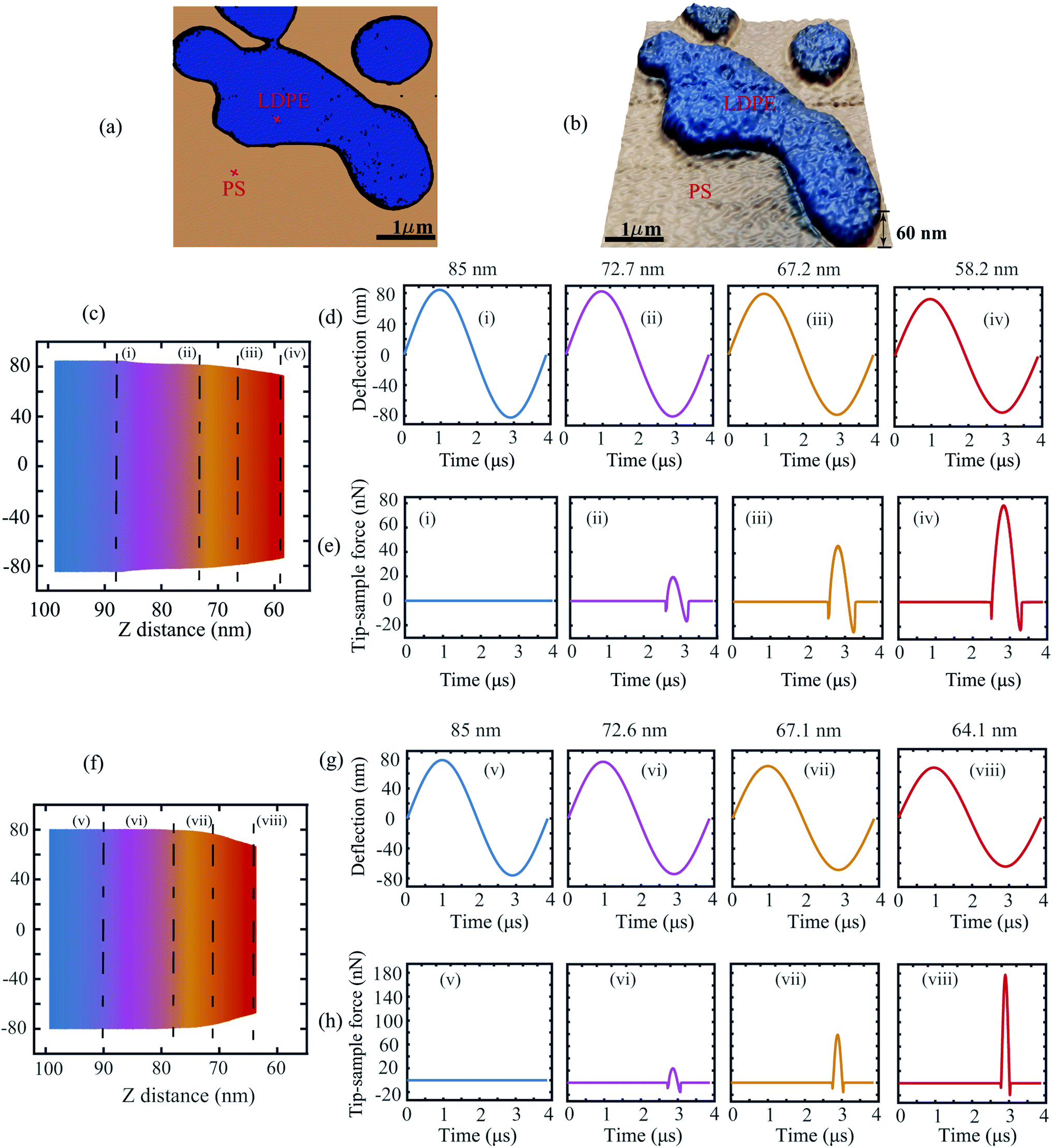 | ||
| Fig. 4 Data-driven identification of tip–sample interaction as a function of tip–sample separation on PS-LDPE sample. (a and b) Phase and topography images of PS-LDPE blend sample, respectively. The blue contour indicates the LDPE islands and the orange contour the PS matrix. (c) Experimental dynamic spectroscopy signal obtained with 80% set-point ratio on LDPE material. The dashed lines indicate specific tip–sample distances at which data-driven identification is performed. The distances as read from left to right are at 85 nm, 72.7 nm, 67.2 nm, 58.2 nm, respectively. (d) Experimental deflection signal obtained from averaging 15 periods at different tip–sample sample distances. (e) Identification of tip–sample force based on the data-driven model at different tip–sample distances. (f) Experimental dynamic spectroscopy signal obtained with 80% set-point ratio on PS material. The dashed lines indicate specific tip–sample distances at which data-driven identification is performed. The distances as read from left to right are at 85 nm, 72.6 nm, 67.1 nm, 64.1 nm, respectively. (g) Experimental deflection signal obtained from averaging 15 periods at different tip–sample distances. (h) Identification of the tip–sample force based on data-driven model at different tip–sample sample distances. | ||
It can be observed that at 85 nm the cantilever is initially in a state of no-interaction far away from the sample (Fig. 4(d(i))) and thus the corresponding tip–sample force is zero as indicated by the blue curve. As the cantilever is brought closer to the sample, the amplitude of the deflection signal drops (Fig. 4(d(ii)–(iv))) owing to the presence of tip–sample forces and thus the interaction force gradually increases as shown in Fig. 4(e(ii)–(iv)). A similar trend is observed for the PS sample in Fig. 4(f)–(h).
Tip–sample contact analysis
In the experimental results shown in Fig. 4(e) and (h) the tip–sample force appears as a clipped sine wave whose magnitude depends on the contact duration, i.e. pulse width. The contact span, in turn, depends on the effective stiffness of the cantilever-sample configuration. For compliant samples such as LDPE, we expect a larger contact duration and thus a broadly distributed tip–sample force.47 In contrast, we expect a faster increase in tip–sample force on stiffer PS sample since larger forces are required to produce a given depth of indentation in these samples.47,48 This results in a shorter duration of the contact with a narrower waveform of the tip–sample force.12 Our machine learning algorithm captures these underlying features accurately in both samples without any prior assumption on the nature of the interaction.Furthermore, by analyzing the interaction exponent of functions that describe the indentation of the tip into the sample, we show that the interaction geometry follows a cone indenting a flat geometry as opposed to the commonly used sphere-half-plane model. The tip–sample interaction in dynamic AFM is mathematically described by power-law relations.49 In particular, several studies in contact mechanics have shown that the indentation force and the indentation depth are linked by a nonlinear function that depends not only on the material properties but also on the geometry of the AFM tip and the sample being investigated. This prompted the force reconstruction techniques in dynamic AFM to seek the instantaneous force profiles as a function of tip–sample distance in the form14,47,49
| Find = γδρ, | (3) |
Using our machine learning approach we retrieve ρ from a library containing a collection of functions with varying exponents. Depending on the nature of interaction, our optimization procedure automatically converges to the best value. This is further highlighted in Fig. 5(a), where we plot the histogram of the exponents of the indentation functions chosen directly by the machine learning process. The analysis shows a mean value of ρ = 2.27 ± 0.4 which is in excellent agreement with the values previously reported in different studies.14,47 Adding to this, we extract the effective stiffness value by assuming an interaction exponent of 2.27 and plot the histograms for both PS and LDPE material. The analysis shows a clear distinction in the stiffness value, where the PS material is approximately twelve times stiffer than the LDPE material. This is in agreement with previous measurements and in-line with the expected bulk modulus values of PS and LDPE.13,14,51
 | ||
| Fig. 5 Histograms of conservative tip–sample interaction measurements on PS-LDPE sample. (a) Histograms of the interaction geometry for the PS (red) and LDPE (blue) domains of the sample. (b) Histograms of the stiffness factor for the PS (red) and LDPE (blue) domains of the sample assuming the mean interaction geometry factor of 2.27. The histograms confirm that the PS sample is stiffer than LDPE sample. | ||
Finally, in addition to providing insight into elastic behaviour of the sample, our machine learning approach also predicts the hysteresis in the interaction force due to energy dissipation as an asymmetry in the clipped sine wave (see Fig. 4(e) and (h)). The hysteresis is obtained in both PS and LDPE samples, but similar to previous observations,12,47,52 the dissipation in case of the compliant sample (LDPE) is found to be much larger than PS. Within our function library, the dissipation is linked to lδp-type functions where δ and are the indentation depth and rate of indentation, respectively and the coefficients l and p are material-related interaction exponents. This suggests that the viscoelastic nature of the polymer could be a major contributor to the energy dissipation.1,2,53–55 Our analysis shows the potential of machine learning approaches to overcome some of the inherent short comings of prior methods where complex or ad hoc models are often used to estimate elastic/viscoelastic properties1,56,57 and thus are limited in their ability to accurately represent tip contact with softer, more adhesive and viscoelastic surfaces. In contrast to this, machine learning algorithm can autonomously pick the best functions to represent the experimental data and distill a physically interpretable model that governs the tip–sample dynamics.
Conclusion
In summary, we proposed an approach based on machine learning and data science to predict the nanoscale interaction forces in dynamic AFM measurements. We discussed the training methodology and supervision of the algorithm based on standard AFM models, and explained the model selection criterion in the pareto space via tuning hyper-parameters. We showed that our data-driven algorithm captures the governing equations and the tip–sample interaction force on numerically generated data with an accuracy of more than 90%. To highlight the utility of our approach, we also performed several experiments on softer LDPE and stiffer PS polymeric samples and estimated the nanoscale interaction force with high resolution. Additionally, we showed that our approach can also distinguish the different polymeric samples based on their elasticity and further provide insight into the energy dissipation, hysteresis as well as the tip geometry during contact.The results from our study are inline with the findings previously reported from AFM measurements of polymers. This further illustrates the potential of machine learning and data-driven methodologies to uncover the true physics of the tip–sample interaction in materials at the nanoscale without any prior assumption on the mathematical models to estimate surface forces. The results further highlight the inherent sub-microsecond temporal resolution and nano-Newton peak loading forces expected in dynamic AFM and facilitate high resolution mapping of nanomechanical properties. In addition to estimating the sample properties, by taking advantage of future generations of high-frequency force sensors, acquisition electronics and data processing algorithms, we envision that data science combined with machine learning techniques will uncover the true potential of dynamic AFM in understanding the physics behind transient biological processes, developing novel feedback architectures and high-resolution dynamical force–volume measurements at video rate.
Methods
Experimental setup
The experiments are performed using a commercial AFM (JPK Nanowizard) and a multi-lock-in amplifier from Intermodulation products58 that can function as a Field Programmable Gated Array (FPGA) that collects and analyzes the cantilever deflection data. We used a commercially available rectangular silicon cantilever (TAP300AL-G, Budgetsensors) and a two-component polymer blend made up of Polystyrene (PS) and Low Density Polyethylene (LDPE) (from Bruker) to perform the experiments. For each experiment, the spring constant of the cantilever (k = 20.68 N m−1), its resonance frequency (f0 = 259.9 kHz), and quality factor (Q = 443) are determined using the thermal calibration method.59The time signal of the cantilever interacting with the polymer sample is captured by implementing a procedure which uses standard modalities available in commercial AFM. As a first step, we perform standard dynamic spectroscopy operation at a specific set point ratio comparable with the ratios used in normal scanning operation in dynamic AFM. The AFM is then synchronized with the FPGA using a trigger signal to ensure a one-to one-correlation between the time axis and the tip–sample distance measurements. Next, the resulting change in vibrational amplitude is recorded using the built in lock-in amplifier within the AFM and using the FPGA at 50 MHz, simultaneously. In this way, we capture the lock-in amplitude and phase data as well as the real-time motion of the cantilever as a function of the varying tip–sample distance.
In the next step, the experimental data obtained by the FPGA is post-processed to align the deflection versus time signal with that of the lock-in amplitude versus tip–sample distance signal extracted from the AFM. This step correlates to access chunks of time data corresponding to specific tip–sample separations. Finally, the deflection signal is de-noised and differentiated using Savitzky–Golay filter to obtain all three state vector channels, namely acceleration, velocity, and time. The Savitzky–Golay filter uses least squares approximation to smoothen noisy experimental measurements without distorting the underlying signal as well as suppresses the high frequency noise in the signal.41,42
Choice of hyper-parameters for the algorithm
The data-driven algorithm requires the specification of two parameters, ν and λ that control the learning process. The parameter ν controls the strength of relaxation for the coefficient matrix W and how closely it matches Ξ. A larger value of ν allows for larger relaxation and vice versa. Whereas, the parameter λ controls the strength of regularization. In our analysis we use a l0 regularization which is equivalent to hard-thresholding, making the optimization problem non-convex. The l0 norm will threshold coefficients below a value determined by both ν and λ. For example, if the desired threshold value is called η then the value of λ is chosen via the relationship λ = η2/2ν.47We note that it is often difficult to know the desired threshold value a priori for every AFM experiment; hence we performed extensive simulations and experiments and based on the analysis we observed that for the best results in a dynamic AFM application, it is a good starting point to use η = 1/Q, where, Q is the quality factor of the cantilever. By normalizing the dynamical system with the correct length and time scales it is possible to make Q the smallest identifiable coefficient in the equation of motion, thus making it the ideal candidate as a threshold parameter. Furthermore, we extend the parameter range by allowing a tolerance of 15% and utilize the hyper-opt python package to determine the best threshold coefficient that results in the smallest possible equation of motion via cross validation.
Choice of constraints for the algorithm
The physics informed constraints that must be imposed to determine the governing equations are obtained from experimental conditions. In particular, we obtain information on the stiffness (k), quality factor (Q) and the resonance frequency (f0) of the cantilever directly from the experiments by performing a thermal calibration procedure.59 In addition to these information, a final constraint on the amplitude of excitation is required. This is crucial for performing accurate system identification since the amplitude of the forcing function Fc (dither piezo based excitation) remains constant while the cantilever approaches the sample and thus the reduction in the amplitude should be purely attributed to the tip–sample interaction force. Therefore, a constraint on the amplitude of base excitation will force the algorithm to select the right nonlinear functions that can accommodate this amplitude reduction.We derive the constraint on Fc by performing an intermediate identification step on what we refer to as no-interaction data. The no-interaction data are obtained far from the sample and as the name suggests have no influence from the tip–sample forces. These data-sets are similar to free air vibration in an experimental scenario and this intermediate step can be viewed as fitting the free air vibration data with a simple harmonic oscillator to estimate the excitation amplitude. Based on these information, we then introduce our constraints into the data-driven algorithm by assuming the governing equation of the cantilever to be of the form:
 | (4) |
| D = Q−1 |
| K = k |
| B = Fc |
These constraints can be more intuitively understood by looking at the function library below.
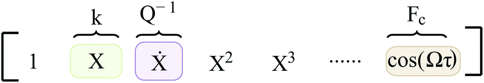
Here, the coefficient of function X which co-relates to the deflection of the cantilever is given by stiffness k, the function describing the velocity of the cantilever (Ẋ) has its coefficient dictated by the inverse of the quality factor (Q) and finally the function governing the amplitude of excitation (cos(Ωτ)) by Fc. Furthermore, during the model discovery, we allow a tolerance of 15% in the aforementioned coefficient values to account for the inconsistencies encountered in the determination of cantilever properties via thermal calibration procedure.
Data availability
The authors declare that all the data in this manuscript are available upon request.Author contributions
AC, PB, and FA conceived the experiments. AC fabricated the samples and conducted the experiments; AC, PB, MAB, and FA did data analysis and interpretation. US and FA supervised the project. All the authors jointly wrote the article with main contribution from AC. All authors discussed the results and commented on the article.Conflicts of interest
The authors declare no competing interests.Acknowledgements
This work is part of the research programme ‘A NICE TIP TAP’ with grant number 15450 which is financed by the Netherlands Organisation for Scientific Research (NWO). FA also acknowledges financial support from European Union's Horizon 2020 research and innovation program under Grant Agreement 802093 (ERC starting grant ENIGMA). The authors also acknowledge fruitful discussions with Dr Daniel Forchheimer for FPGA coding.Notes and references
- R. Garcia, C. J. Gomez, N. F. Martinez, S. Patil, C. Dietz and R. Magerle, Phys. Rev. Lett., 2006, 97, 016103 CrossRef CAS PubMed.
- E. T. Herruzo, A. P. Perrino and R. Garcia, Nat. Commun., 2014, 5, 3126 CrossRef PubMed.
- B. Rajabifar, A. K. Bajaj, R. G. Reifenberger, R. Proksch and A. Raman, Nanoscale, 2021, 13, 17428–17441 RSC.
- C. Dietz, M. Schulze, A. Voss, C. Riesch and R. W. Stark, Nanoscale, 2015, 7, 1849–1856 RSC.
- Y. Sugimoto, P. Pou, M. Abe, P. Jelinek, R. Pérez, S. Morita and s. Custance, Nature, 2007, 446, 64–67 CrossRef CAS PubMed.
- C.-Y. Lai, S. Perri, S. Santos, R. Garcia and M. Chiesa, Nanoscale, 2016, 8, 9688–9694 RSC.
- A. J. Page, A. Elbourne, R. Stefanovic, M. A. Addicoat, G. G. Warr, K. Voïtchovsky and R. Atkin, Nanoscale, 2014, 6, 8100–8106 RSC.
- A. Raman, S. Trigueros, A. Cartagena, A. P. Stevenson, M. Susilo, E. Nauman and S. A. Contera, Nat. Nanotechnol., 2011, 6, 809–814 CrossRef CAS PubMed.
- S. Benaglia, V. G. Gisbert, A. P. Perrino, C. A. Amo and R. Garcia, Nat. Protoc., 2018, 13, 2890–2907 CrossRef CAS PubMed.
- M. Krieg, G. Fläschner, D. Alsteens, B. M. Gaub, W. H. Roos, G. J. L. Wuite, H. E. Gaub, C. Gerber, Y. F. Dufrêne and D. J. Müller, Nat. Rev. Phys., 2019, 1, 41–57 CrossRef.
- O. Sahin, S. Magonov, C. Su, C. F. Quate and O. Solgaard, Nat. Nanotechnol., 2007, 2, 507 CrossRef PubMed.
- K. Gadelrab, S. Santos, J. Font and M. Chiesa, Nanoscale, 2013, 5, 10776–10793 RSC.
- A. F. Payam, D. Martin-Jimenez and R. Garcia, Nanotechnology, 2015, 26, 185706 CrossRef PubMed.
- D. Platz, D. Forchheimer, E. A. Tholen and D. B. Haviland, Nat. Commun., 2013, 4, 1360 CrossRef PubMed.
- H. Shuiqing and R. Arvind, Nanotechnology, 2008, 19, 375704 CrossRef PubMed.
- H. Hölscher, Appl. Phys. Lett., 2006, 89, 123109 CrossRef.
- M. Stark, R. W. Stark, W. M. Heckl and R. Guckenberger, Proc. Natl. Acad. Sci., 2002, 99, 8473–8478 CrossRef CAS PubMed.
- E. Couderc, Nat. Energy, 2018, 3, 85 CrossRef.
- L. Hervé, D. C. A. Kraemer, O. Cioni, O. Mandula, M. Menneteau, S. Morales and C. Allier, Sci. Rep., 2020, 10, 20207 CrossRef PubMed.
- S. Yang, S. W. K. Wong and S. C. Kou, Proc. Natl. Acad. Sci., 2021, 118, e2020397118 CrossRef CAS PubMed.
- A. P. Nievergelt, N. Banterle, S. H. Andany, P. Gonczy and G. E. Fantner, Nat. Nanotechnol., 2018, 13, 696–701 CrossRef CAS PubMed.
- M. Dong and O. Sahin, Nat. Commun., 2011, 2, 247 CrossRef PubMed.
- M. Shibata, H. Yamashita, T. Uchihashi, H. Kandori and T. Ando, Nat. Nanotechnol., 2010, 5, 208–212 CrossRef CAS PubMed.
- P. Hinterdorfer and Y. F. Dufrêne, Nat. Methods, 2006, 3, 347–355 CrossRef CAS PubMed.
- R. Garcia and E. T. Herruzo, Nat. Nanotechnol., 2012, 7, 217–226 CrossRef CAS PubMed.
- S. Santos, C.-Y. Lai, T. Olukan and M. Chiesa, Nanoscale, 2017, 9, 5038–5043 RSC.
- Y. F. Dufrene, T. Ando, R. Garcia, D. Alsteens, D. Martinez-Martin, A. Engel, C. Gerber and D. J. Muller, Nat. Nanotechnol., 2017, 12, 295 CrossRef CAS PubMed.
- S. I. Lee, S. W. Howell, A. Raman and R. Reifenberger, Ultramicroscopy, 2003, 97, 185–198 CrossRef CAS PubMed.
- A. Chandrashekar, P. Belardinelli, S. Lenci, U. Staufer and F. Alijani, Phys. Rev. Appl., 2021, 15, 024013 CrossRef CAS.
- S. L. Brunton, J. L. Proctor and J. N. Kutz, Proc. Natl. Acad. Sci., 2016, 113, 3932–3937 CrossRef CAS PubMed.
- J. Sotres, H. Boyd and J. F. Gonzalez-Martinez, Nanoscale, 2021, 13, 9193–9203 RSC.
- K. Champion, P. Zheng, A. Y. Aravkin, S. L. Brunton and J. N. Kutz, IEEE Access, 2020, 8, 169259–169271 Search PubMed.
- P. Zheng, T. Askham, S. L. Brunton, J. N. Kutz and A. Y. Aravkin, IEEE Access, 2019, 7, 1404–1423 Search PubMed.
- N. M. Mangan, S. L. Brunton, J. L. Proctor and J. N. Kutz, IEEE Trans. Mol. Biol. Multi-Scale Commun., 2016, 2, 52–63 Search PubMed.
- S. Santos, C.-Y. Lai, C. A. Amadei, K. R. Gadelrab, T.-C. Tang, A. Verdaguer, V. Barcons, J. Font, J. Colchero and M. Chiesa, Nanoscale, 2016, 8, 17400–17406 RSC.
- B. Huang, Z. Li and J. Li, Nanoscale, 2018, 10, 21320–21326 RSC.
- N. M. Mangan, T. Askham, S. L. Brunton, J. N. Kutz and J. L. Proctor, Proc. R. Soc. A, 2019, 475, 20180534 CrossRef CAS PubMed.
- B. M. de Silva, K. Champion, M. Quade, J.-C. Loiseau, J. N. Kutz and S. L. Brunton, J. Open Source Softw., 2020, 5, 2104 CrossRef.
- B. Derjaguin, V. Muller and Y. Toporov, J. Colloid Interface Sci., 1975, 53, 314–326 CrossRef CAS.
- K. L. Johnson, K. Kendall, A. D. Roberts and D. Tabor, Proc. R. Soc. A, 1971, 324, 301–313 CAS.
- A. Savitzky and M. J. E. Golay, Anal. Chem., 1964, 36, 1627–1639 CrossRef CAS.
- M. A. Bessa, J. T. Foster, T. Belytschko and W. K. Liu, Comput. Mech., 2014, 53, 1251–1264 CrossRef.
- A. Chandrashekar, P. Belardinelli, S. Lenci, U. Staufer and F. Alijani, Phys. Rev. Appl., 2021, 15, 024013 CrossRef CAS.
- E. Solak, R. Murray-Smith, W. E. Leithead, D. J. Leith and C. E. Rasmussen, NIPS, 2002, 15, 1033–1040 Search PubMed.
- M. Raissi, P. Perdikaris and G. E. Karniadakis, J. Comput. Phys., 2017, 335, 736–746 CrossRef.
- L. I. Rudin, S. Osher and E. Fatemi, Phys. D, 1992, 60, 259–268 CrossRef.
- O. Sahin, C. F. Quate, O. Solgaard and F. J. Giessibl, in Handbook of Nanotechnology, Springer, 2010, pp. 711–729 Search PubMed.
- O. Sahin, Phys. Rev. B: Condens. Matter Mater. Phys., 2008, 77, 115405 CrossRef.
- J. N. Israelachvili, Intermolecular and Surface Forces, Academic Press, 3rd edn, 2011 Search PubMed.
- K. L. Johnson, Contact Mechanics, Cambridge University Press, 1985 Search PubMed.
- O. Sahin and N. Erina, Nanotechnology, 2008, 19, 445717 CrossRef PubMed.
- S. Santos, K. R. Gadelrab, T. Souier, M. Stefancich and M. Chiesa, Nanoscale, 2012, 4, 792–800 RSC.
- H. V. Guzman, A. P. Perrino and R. Garcia, ACS Nano, 2013, 7, 3198–3204 CrossRef CAS PubMed.
- C.-Y. Lai, T. Olukan, S. Santos, A. Al Ghaferi and M. Chiesa, Chem. Commun., 2015, 51, 17619–17622 RSC.
- P. D. Garcia, C. R. Guerrero and R. Garcia, Nanoscale, 2020, 12, 9133–9143 RSC.
- D. B. Haviland, C. A. van Eysden, D. Forchheimer, D. Platz, H. G. Kassa and P. Leclère, Soft Matter, 2015, 12, 619–624 RSC.
- P.-A. Thorén, R. Borgani, D. Forchheimer, I. Dobryden, P. Claesson, H. Kassa, P. Leclère, Y. Wang, H. Jaeger and D. Haviland, Phys. Rev. Appl., 2018, 10, 024017 CrossRef.
- D. Platz, E. A. Tholen, D. Pesen and D. B. Haviland, Appl. Phys. Lett., 2008, 92, 153106 CrossRef.
- J. E. Sader, J. W. M. Chon and P. Mulvaney, Rev. Sci. Instrum., 1999, 70, 3967–3969 CrossRef CAS.
Footnote |
| † Electronic supplementary information (ESI) available. See https://doi.org/10.1039/d2na00011c |
| This journal is © The Royal Society of Chemistry 2022 |