Prediction of atomic stress fields using cycle-consistent adversarial neural networks based on unpaired and unmatched sparse datasets

Abstract

Deep learning holds great promise for applications in materials science, including the discovery of physical laws and materials design. However, the availability of proper data remains a challenge – often, data lacks labels, or does not contain direct pairing between input and output property of interest. Here we report an approach based on an adversarial neural network model – composed of four individual deep neural nets – to yield atomistic-level prediction of stress fields directly from an input atomic microstructure, illustrated here for defected graphene sheets under tension. The primary question we address is whether it is possible to predict stress fields without any microstructure-to-stress fields pairings, nor the existence of any input–output pairs whatsoever, in the dataset. Using a cycle-consistent adversarial neural net with either U-Net, ResNet and a hybrid U-Net-ResNet architecture, applied to a system of graphene lattices with defects we devise an algorithmic framework that enables us to successfully train and validate a model that reliably predicts atomistic-level field data of unknown microstructures, generalizing to reproduce well-known nano- and micromechanical features such as stress concentrations, size effects, and crack shielding. In a series of validation analyses, we show that the model closely reproduces reactive molecular dynamics simulations but at significant computational efficiency, and without a priori knowledge of any physical laws that govern this complex fracture problem. The model opens an avenue for upscaling where the mechanistic insights, and predictions from the model, can be used to construct analyses of very large systems, based off relatively small and sparse datasets. Since the model is trained to achieve cycle consistency, a trained model features both forward (microstructure to stress) and inverse (stress to microstructure) generators; offering potential applications in materials design to achieve a certain stress field. Another application is the prediction of stress fields based off experimentally acquired structural data, where the knowledge of solely positions of atoms is sufficient to predict physical quantities for augmentation or analysis processes.

---

1. Introduction

Predicting stress, strain and other field data in complex nanomaterials under varied boundary conditions such as mechanical stress is a critical aspect of nanoscience and nanotechnology.^1–3 While methods exist to predict field data, such as atomistic simulation, these can be costly and ineffective if applied to a very large number of microstructural variations, e.g. to extract fundamental physical insights from data, or in inverse problems or materials discovery tasks. Here we report a deep learning-based method to solve this problem with applications in both multiscale modeling as well as experimental analysis, applied here to graphene with defects exposed to mechanical loading. While this system is chosen as a representative system, the method reported here is generally applicable to other nanomaterials, other field data, and other settings, including perhaps in distinct sets of other physical phenomena.

Machine learning broadly, and especially deep learning^4,5 holds great promise for applications in nanoscience, including materials discovery and design,^6–9 and has been applied to various nanoscale systems including to graphene in prior research.^10,11 Here we explore the analysis of graphene mechanics using deep learning, applied specifically to the nanomechanical problem of fracture mechanics,^12,13 using an adversarial framework. Earlier work has shown that field data can accurately be predicted by training neural networks against paired images^14,15 (that is, neural networks are given pairs of input and output fields during during).

While paired datasets (e.g. field images) may be available in some cases, there are scenarios where such pairings, or the knowledge of pairings, may not exist, such as in broad experimental data collection or in the combination of data from multiple sources. Importantly, we believe it is also a question of fundamental interest to assess whether correct field-to-field predictions, including combining multiple objectives such as displacement fields and stress fields simultaneously, can be predicted from datasets without the existence of pairs in the dataset. We address this fundamental question in this study and show that it is indeed possible to solve such a problem through the use of an adversarial training approach, offering a game theoretic approach to solve this nanomechanics problem.

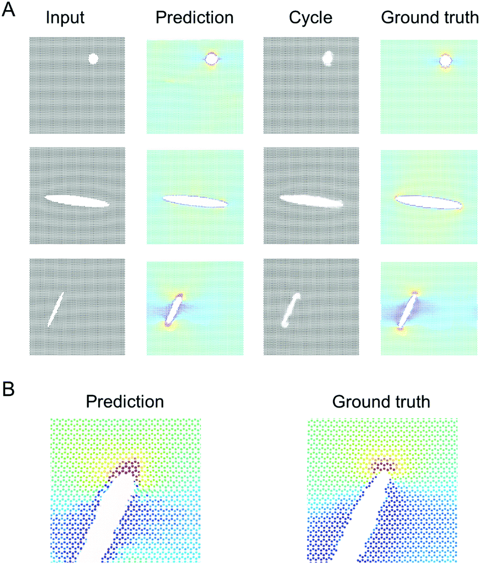
Fig. 1 shows the model setup used in this study, resembling a small piece of graphene under periodic boundary conditions and uniaxial loading.¹⁶Fig. 1A shows the model setup and application of mechanical strain, used here for demonstration of the method, and Fig. 1B depicts sample results from molecular dynamics simulations that serve as input to train the deep learning model (left panel: input microstructure, right panel: predicted output stress field where numerical stress values in each atom are mapped to a color via a colormap; as predicted from MD simulation). We solve both the forward problem (predicting stress fields from microstructure) as well as the inverse problem (predicting microstructure from stress field). The model does not require any pairing of input–output images, and that it works for datasets that do not even feature the existence of any pairs in the dataset.

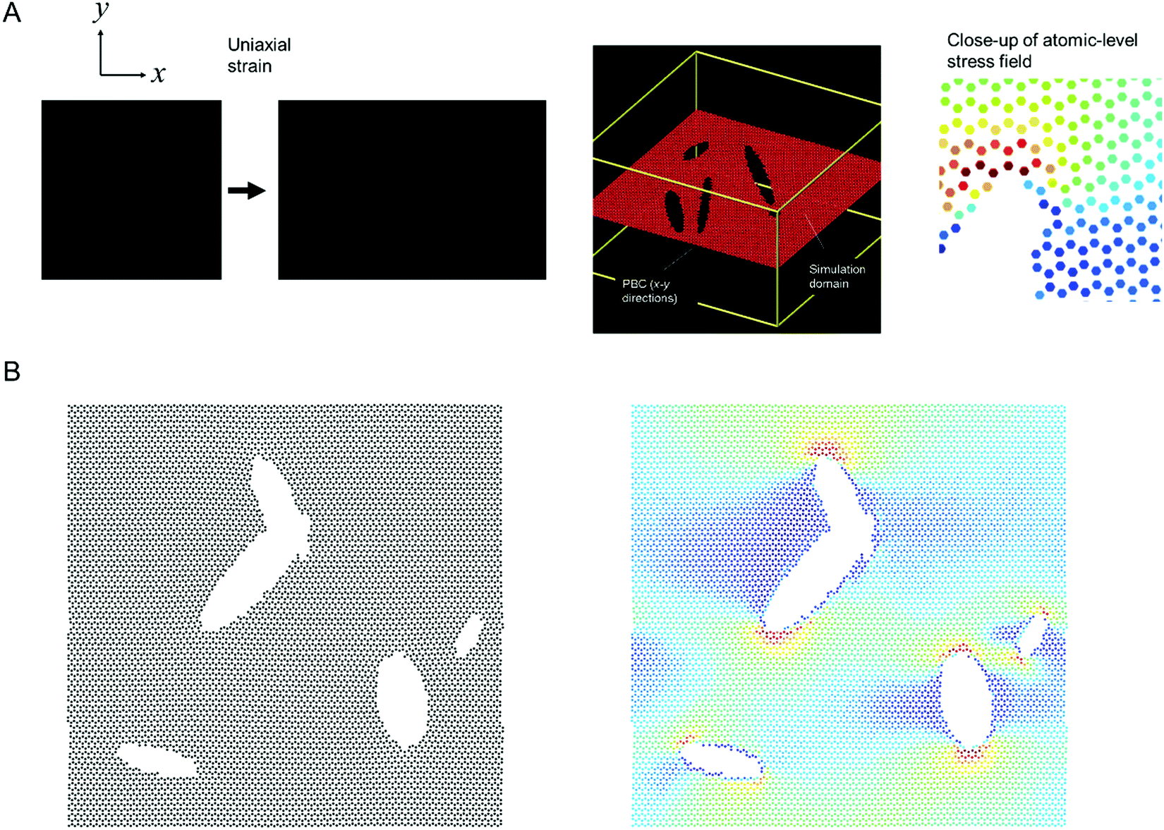Fig. 1 Atomistic simulation setup (Panel A, strain in the x-direction is exaggerated for clarity) and sample results from the MD simulations (left: microstructure, right: stress field). All MD simulations are carried out in LAMMPS.¹⁷ We solve both the forward problem (predicting stress fields from microstructure) as well as the inverse problem (predicting microstructure from stress field). The stress field images are generated by mapping a stress value (or other field data) to a color; and the process can be reversed when converting a predicted field back into numerical field data for further analysis.

2 Results and discussion

Following the overall setup depicted in Fig. 1, our goal is to predict stress fields from an input lattice structure that features various types of defects, and vice versa.^18,19 The deep learning model is trained on MD simulation data (details in Materials and methods).

Fig. 2 depicts the training set design without any pairs (see “X” marked in Fig. 2A to note the images removed, for just a few sample images), and also no pairing information between input and output data. Fig. 2B depicts a sample of the collection of input microstructures and output stress fields. The van Mises stress²⁰ is used here as an effective overall stress measure, but the method can be generalized for other field data. Two types of crack simulations are included, graphene sheets with single cracks (left half) and multiple cracks (right half). We conduct a total of 2000 MD simulations, half with single cracks and the other half with multiple cracks, for a total of 4000 images to begin with. Once any pairs are removed, a total of 2000 images are left in the training set (this is reduced to 1000 images for training to test the reliability of the method with even fewer images).

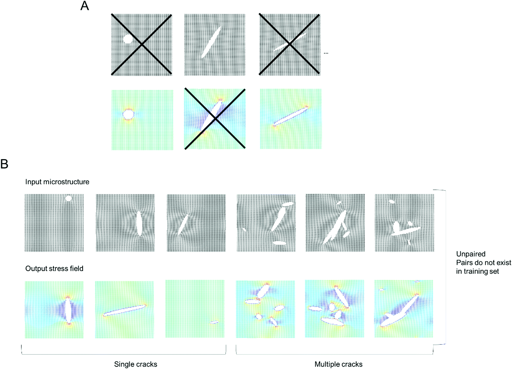Fig. 2 Training set design without pairing and without pairs (panel A) and overview of the types of data used (selection) (panel B). The training set includes a collection of input microstructures and resulting output stress fields (van Mises stress used here, but the method can be generalized for other field data). The dataset used here consists of unpaired images, and pairs of input–output combinations are not included either. Two types of crack simulations are included, single cracks (left half) and multiple cracks (right half). We conduct a total of 2000 simulations, half with single cracks and the other half with multiple cracks. All pairs are removed, leaving a total of 2000 images in the training set (reduced to 1000 images for training to test the reliability of the method with even fewer images).

We use a cycle-consistent adversarial neural net (GAN),^21,22 as shown in Fig. 3. Fig. 3 shows an overview of the models, featuring U-Net, ResNet and hybrid U-Net-ResNet generators,^23,24 as well as two PatchGAN classifiers.^25,26 Generator G transforms input lattices into stress fields and generator F transforms stress fields into input lattices. Using adversarial training, G learns to generate images that resemble real stress fields, and a discriminator D_y, aims to distinguish between generated stress fields x̃ = G(x_{microstructure}) and real stress fields x_stress. At the same time, F learns to generate images that resemble real stress fields, and a discriminator D_x aims to distinguish between generated microstructures x̃_{microstructure} = F(x_stress) and real microstructures x_{microstructure}.

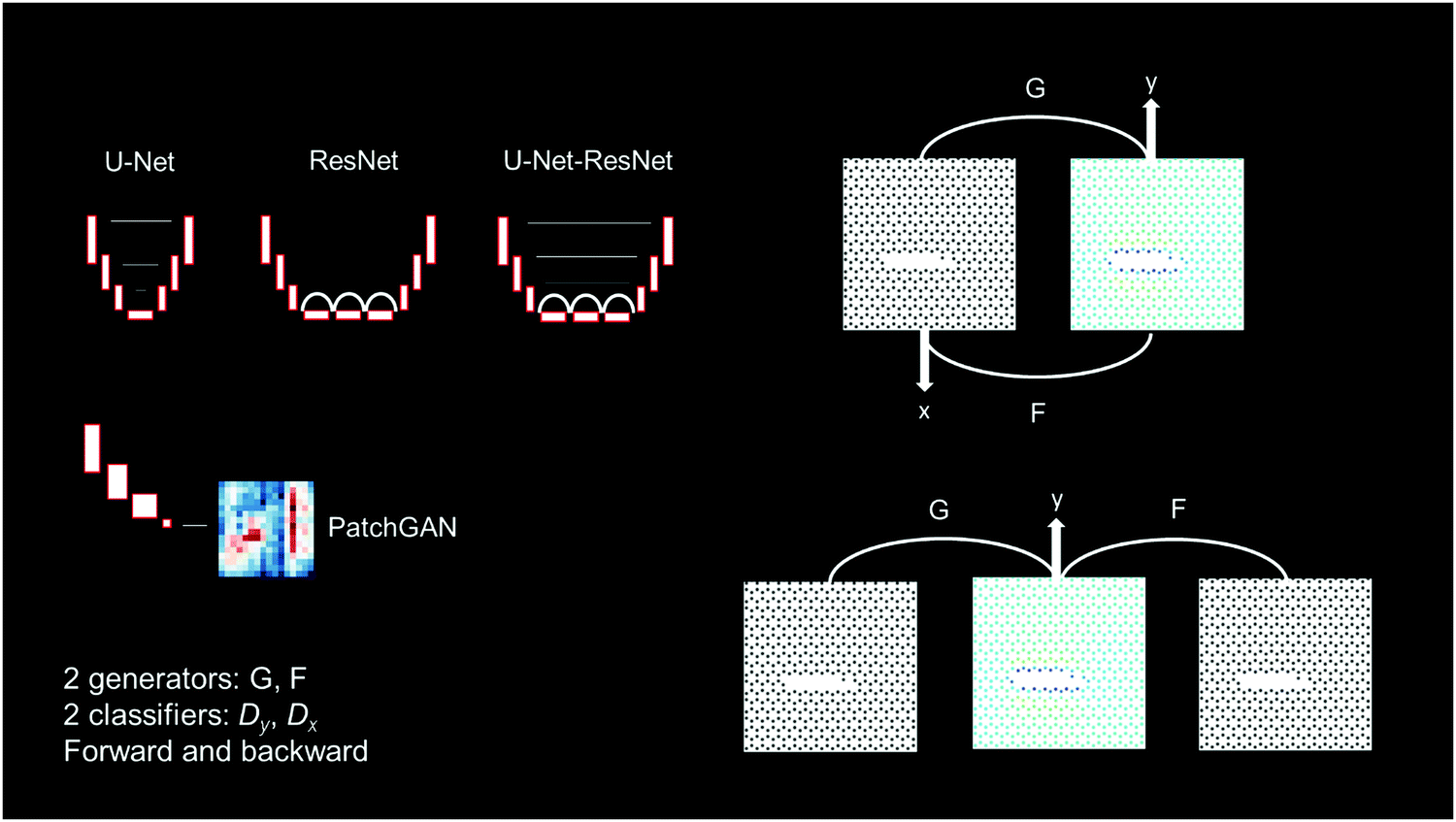Fig. 3 Overview of the cycle consistent neural network models, featuring U-Net, ResNet and hybrid U-Net-ResNet generators, as well as 2 PatchGAN classifiers (same structure in all models used). Generator G transforms input lattices into stress fields and generator F transforms stress fields into input lattices. Classifiers D_y and D_x are trained to determine whether generated stress fields or microstructures are real or fake. In the adversarial training of this cycle consistent neural network, the generator gets better and better at producing realistic stress fields that can no longer be distinguished from real ones (and vice versa, for the microstructures). Due to the cycle consistent formulation of the losses, no pairings of the input and output are necessary.

With x_i and x̃_i denoting the real field and approximate, predicted field, respectively,

G(x_{microstructure}) = x̃_stress (1)

and

F(x_stress) = x̃_{microstructure} (2)

Classifiers D_y/D_x are trained to determine whether microstructures/stress fields are real or fake. In the adversarial training of this cycle consistent neural network, the generator gets better and better at producing realistic stress fields that can no longer be distinguished from real ones (and vice versa). This is because we train the model to feature cycle consistency in both forward and backward direction, that is:

F(G(x_{microstructure})) = x̃_{microstructure} ≈ x_{microstructure} (3)

and

G(F(x_stress)) = x̃_stress ≈ x_stress. (4)

We also train the model to ensure identity loss, that is,

F(x_{microstructure}) = x̃_{microstructure} ≈ x_{microstructure} (5)

and

G(x_stress) = x̃_stress ≈ x_stress (6)

Eqn (5) and (6) signify that if a real stress field is provided to generator G, the same stress field is produced. Similarly, once an input lattice is provided to F, the same input lattice is produced.

In other words, if we provide a microstructure to generator G we will get the “same” microstructure back. Similarly, if we provide a stress field to generator F will get the “same” stress field back.

A λ parameter is introduced to weigh the relative contributions of the losses (discriminator loss, cycle consistency loss, and identity loss). Cycle consistency losses are weight by λ_cycle, and the identity loss by λ_identity. These two contributions are typically weighted at λ_i ≫ 1 (details in Materials and methods). This strategy ensures that the model not only learns how to generate images that “look like” the required output, but specifically requires that the mapping in both forward and backward direction is satisfied. This is critical for a physical problem as solved here.

Indeed, we hypothesize that due to the cycle consistent formulation of the model, no pairings of the input and output are necessary, and that the model can even learn how to predict multiple features at the same time.

We explore the use of two types of generator models, one based on a U-Net architecture, and one based on a ResNet architecture (as well as a hybrid model of the two, referred to as U-Net-ResNet). As is shown in the following sections, both models can learn to predict stress fields from input microstructures well, and also solve the inverse problem. Further details on the discriminator models are provided in Materials and Methods, along with other specifics, as well as²² for additional model aspects.

2.1 Results based on the U-Net architecture

Fig. 4 shows results using the U-Net architecture. Fig. 4A shows the generator loss and discriminator loss functions, respectively. Panel B depicts a few sample results, for two distinct inputs (top: microstructure, bottom: stress field). The cycle prediction, comparing to the input, indicates that cycle consistency has been achieved.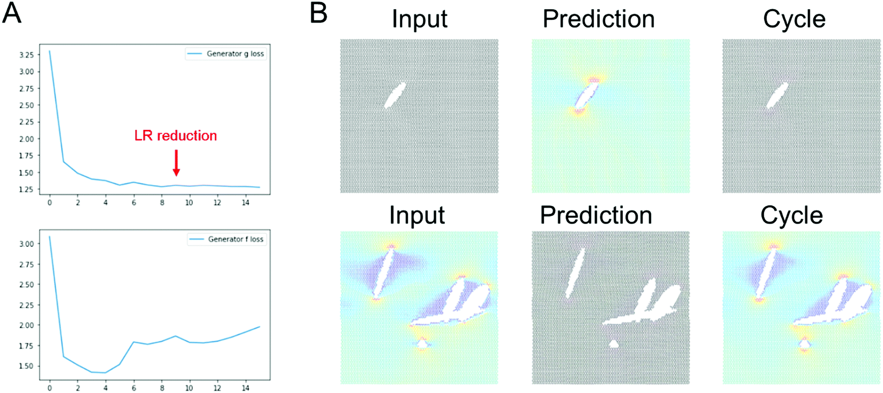

Fig. 4 Results using the U-Net architecture. Panel A shows the generator loss and discriminator loss functions, respectively. Panel B depicts a few sample results, for two distinct inputs (top: microstructure, bottom: stress field). The cycle prediction, comparing to the input, indicates that cycle consistency has been achieved. Note, as shown in Panel A, we reduce the learning rate from 2 × 10⁻⁴ to 2.5 × 10⁻⁵ after 9 epochs.

We now validate the method by comparing predictions for novel microstructures (which have not been part of the training set) with MD simulation results, as shown in Fig. 5. Sample results for single cracks (top 3) and multiple cracks (bottom 3), comparing the input, stress field, cycle, and ground truth, for the U-Net architecture, confirm excellent agreement. It is evident that the model predicts the stress fields very well, generally. As anticipated from fracture mechanics theory,¹³ high stresses occur at crack tips. The model also adequately captures size effects, where smaller cracks lead to lower stress intensity.²⁷ Another interesting result is that the model predicts crack shielding (e.g. bottom example in Fig. 5), and can accurately account for the orientation of the crack, following closely the prediction by Inglis.²⁸ Specifically, the model predicts that horizontal cracks have lower stress concentration than vertically oriented cracks.

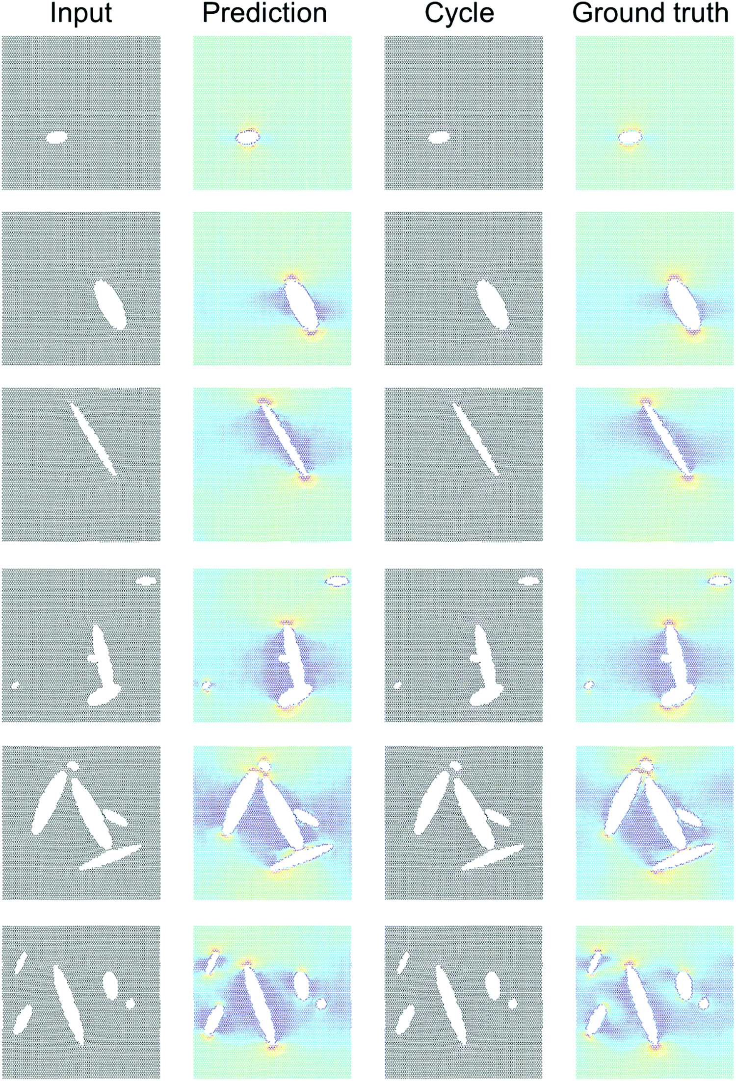Fig. 5 Sample results for single cracks (top 3) and multiple cracks (bottom 3), comparing the input, stress field, cycle, and ground truth, for the U-Net architecture, for validation of the model. The model predicts the stress fields very well, generally, predicting high stresses at crack tips, size effects (smaller cracks lead to lower stress intensity), crack shielding (e.g. bottom example), and orientation of the crack (horizontal cracks have lower stress concentration than vertically oriented cracks). This analysis confirms that x̃_stress ≈ x_stress.

2.2 Results based on the ResNet architecture

Fig. 6 shows results using the ResNet architecture. Fig. 6A shows the generator loss and discriminator loss functions, respectively. Fig. 6B depicts a few sample results, for two distinct inputs (top: microstructure, bottom: stress field). The cycle prediction, comparing to the input, indicates that cycle consistency has been achieved and that the model is capable of solving the inverse problem.

Fig. 6 Results using the ResNet architecture. Panel A shows the generator loss and discriminator loss functions, respectively. Panel B depicts a few sample results, for two distinct inputs (top: microstructure, bottom: stress field). The cycle prediction, comparing to the input, indicates that cycle consistency has been achieved.

Fig. 7 shows sample results for single cracks (top 3) and multiple cracks (bottom 3), comparing the input, stress field, cycle, and ground truth, for the ResNet architecture. As the U-Net model described in the previous section, the ResNet model predicts the stress fields very well, generally, predicting high stresses at crack tips, size effects (smaller cracks lead to lower stress intensity), crack shielding (e.g. bottom example), and orientation of the crack (horizontal cracks have lower stress concentration than vertically oriented cracks).

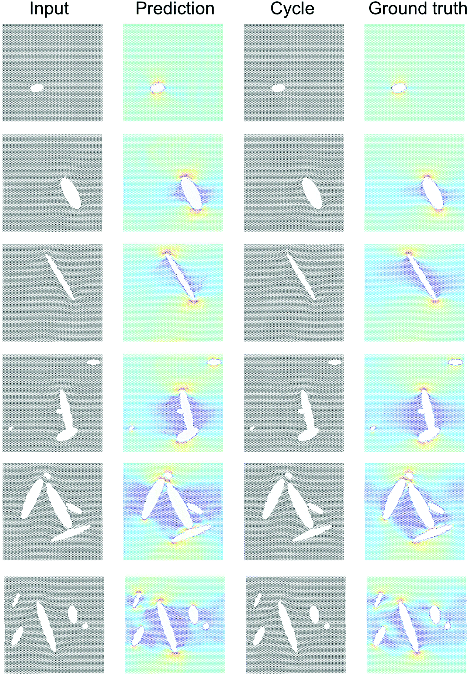Fig. 7 Validating the model against molecular dynamics results. Sample results for single cracks (top 3) and multiple cracks (bottom 3), comparing the input, stress field, cycle, and ground truth, for the ResNet architecture. The model predicts the stress fields very well, generally, predicting high stresses at crack tips, size effects (smaller cracks lead to lower stress intensity), crack shielding (e.g. bottom example), and orientation of the crack (horizontal cracks have lower stress concentration than vertically oriented cracks). This analysis confirms that x̃_stress ≈ x_stress.

It is noted that the ResNet model requires longer training to reach good predictions. It usually took around a few tens of epochs for convergence of the ResNet models, whereas the U-Net model converges within a few epochs.

2.3 Near-crack tip field predictions

Fig. 8 shows a detailed comparison of stresses near crack tip, comparing U-Net, ResNet and ground truth as obtained from MD simulations. Generally, the stress concentration is predicted well at the atomic level, albeit there are some slight differences. The U-Net model tends to make slightly better predictions. Further work is necessary to explore the capacity of both models to make predictions based on different size training sets, noise in the dataset, or other parameters.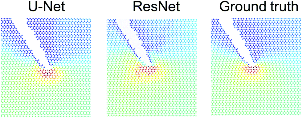

Fig. 8 Validating the model against molecular dynamics results. This figure depicts a detailed comparison of stresses near crack tip, comparing U-Net, ResNet and ground truth. Generally, the stress concentration is predicted well at the atomic level, albeit there are some slight differences. The U-Net model tends to make slightly better predictions (note, Fig. S2 (ESI†) shows a direct comparison between U-Net and ResNet of the entire field; not repeated here since the images are already included in prior figures).

2.4 Predicting field data and displacements simultaneously

In the preceding examples, predictions of the field data was based on input microstructures that did not change configuration (that is, position of atoms) once output fields were added, and hence the model only learned to predict field data without at the same time learning the deformation of the lattice. While this is in principle not limiting since the model can easily learn multiple fields – stress data, displacement data, etc. – and may actually have advantages when using experimental input data of lattices (e.g. in situ images take may already be in deformed state), we now explore whether the model is capable to learn deformations of lattices while at the same time predicting stress fields. We found this to be a much more challenging problem, and hence more difficult to train for, especially for discrete lattice structures as considered here (it is noted in other investigations of continuous field predictions, this problem tends to be easier to solve for, indicating that the discreteness of the lattice poses challenges). While this deserves exploration in future work, we report some results of a successful model that has accomplished this feat, confirming that such models can be developed.

Fig. 9 shows examples from the model that predicts both stress field and deformation simultaneously, using a U-Net-ResNet model (featuring ResNet blocks at the bottom of the “U”, combining the two models used in the previous sections towards a more complex neural network that has the capacity to learn even more complex relationships).

Fig. 9 Validating the model against molecular dynamics results, using a U-Net-ResNet model, while predicting both stress field and deformation simultaneously. Panel A: Comparisons for three sample geometries. The overall shape change of the image is visible, while the stress field is predicted well also. Panel B: Detailed comparison of stresses near crack tip (for the example in the middle), comparing prediction and ground truth. Generally, the overall deformation of the lattice and the atomistic stresses are well reproduced. However, the model fails to accurately convert stress fields into an input microstructure, especially compared to the performance of the other models trained.

Fig. 9A presents comparisons for three sample geometries. The overall shape change of the image is visible, for instance by comparing the input and output shape. Fig. 9B shows a detailed comparison of stresses near crack tip, comparing prediction and ground truth. It can be seen that generally, the stresses are well reproduced. We note that the model failed to accurate learn to predict the input microstructure from an image of a deformed stress field, at least not nearly as good as the earlier models described. This may or may not be considered limiting depending on the objective of the use case, however, it deserves further investigation in future work. For instance, adjusting learning rates and/or relative weights of the losses may help, since the forward vs. backward problems have different complexities associated with them. Other possible explorations in order to achieve better predictions of a deformed lattice to an undeformed lattice include training against solely deformations, not stress fields. We anticipate that some of these questions may be addressed in future work.

3. Conclusion

We reported a deep learning approach to predict atomistic-level field data of unknown microstructure inputs, generalizing to reproduce well-known nano- and micromechanical features such as stress concentrations, size effects, and crack shielding, closely reproducing reactive MD simulations but at significant computational efficiency. A notable feature of the method is that it does not rely on paired images, and that pairs of images do not need to exist in the dataset, at all. We also showed that transfer learning provides a path to solve even more complex problems where not only field data is predicted as a function of an input microstructure, but also deformation fields.

We believe that what has been demonstrated here represents a remarkable feat that offers immense opportunities for many other physical phenomena for which solely “observations”, but absolutely no correlation between the input and output, is known, for mechanistic discovery of accurate pairing by the algorithm itself.

Once the neural net is trained, one of the generators (F to translate microstructures to stress data, and G to translate stress data to microstructures) is sufficient to make relevant predictions. Such predictions can easily be carried out on a CPU or GPU and take a fraction of a second, much less time than a MD simulation to solve the same problem, which can take minutes to hours depending on the size of the system. This is particularly significant when working with complex nanomaterials that require quantum or fully reactive models). It is also noted that transfer learning can be a powerful tool to adapt the model to other scenarios. For instance, a model can be trained against MD simulations as done in this paper and then adapted to learn particularities of a system for which only quantum mechanical data is available. Since transfer learning typically requires much less data, this can be done in a feasible manner, and updating a well-trained neural network only requires a few epochs.

As a more general comment the resulting images of fields produced by the generator neural network can be converted into numerical values by using the color mapping that was used to generate the images from the MD results in the first place (thereby, each color is associated with a particular numerical value). When analyzing a result, the colors predicted by the ML algorithm can be converted into a numerical stress value (or any other field data) by reversing the process, using the same colormap but now mapping a color to a numerical value.

Through these developments we showed that this cycle-consistent GAN model opens an avenue for upscaling – in a multiscale scheme – where the predictions from the model can be used to construct analyses of very large samples, based off relatively small and sparse dataset without any known pairing of input and output, such as by tiling overlapping images generated by smaller “patches” of data, in a sliding fashion. Such sliding algorithms are used in other settings such as image segmentation or image generation,²⁹ and can offer an effective mechanism to create very large-scale high-resolution solutions. Moreover, another application area of the model is the prediction of stress fields based off experimental data, where the knowledge of solely positions of atoms is sufficient to predict physical quantities for augmentation or analysis processes. We note that any model has to be first trained against ground truth data, which includes information about how input and output relate. A possible strategy is to pre-train a model against synthetic data as done in this study, and then use such a model in a fine-tuning step where the model is adapted against another dataset, for instance data generated from experimental imaging.

4. Materials and methods

This section describes detailed methods, including MD simulations, dataset generation, and the neural network model along with training and validation.

4.1 Atomistic simulations and dataset generation

MD simulations to model deformation and fracture of nanomaterials has been widely used for a variety of materials and force fields.^30–32 We consider the geometry shown in Fig. 1A, depicting a graphene lattice with periodic boundary conditions in x-y directions, (cell in the z-direction is much larger to ensure no interactions between images of the single graphene sheet) under uniaxial loading in the x-direction. The interatomic force field is the reactive AIREBO potential,³³ implemented in LAMMPS.¹⁷

The system allows for atomic deformations in x-, y and z-directions (albeit out-of-plane deflections are minimal due to the 2D nature of graphene, especially under tension). To realize a high-throughput LAMMPS simulation setup we first generate an image (black is the background, and white color resembles void regions in cracks or other defects; added using OpenCV image generation functions). The image is then translated into a graphene lattice, where the distribution of atoms and void follows the image colors. The process is automated via a Python script that generates LAMMPS input files, runs LAMMPS, and analyzes the results.

The training set includes both, cases with just single cracks and cases with a larger number of randomly situated cracks, split half. All MD models are carried out using LAMMPS and feature a series of energy minimization using conjugate gradient (CG), MD runs at near-zero temperature, followed by homogeneous strain application (4.5% uniaxial tensile strain applied in the x-direction via a constant strain rate without lateral relaxation until the desired total strain is reached), and then a GG-MD-GC sequence to render an equilibrium stress field. The initial periodic system size before strain application is 170.93 A × 173.95 A. Each of the systems feature around 10 000 carbon atoms (specific number changes due to the existence of defects).

4.1.1 Stress field calculation and dataset. We compute the simulation step averaged atomic von Mises stress σ_von Mises²⁰ in LAMMPS,¹⁷ visualize it using matplotlib, and save images of the input microstructure and the predicted stress fields to generate the data sets. The von Mises stress,²⁰ used here as measure of overall stress as a scalar field, is calculated from the atomic stress tensor σ_ij as:The final training set used for the neural network training is based up to 4000 images total, with 2000 images of input and output, respectively (the input is the lattice without stress field, and the output is the lattice with stress field indicated by color). The complete simulation data is then used to extract the dataset for the training by removing any pairs, to realize a dataset that is (i) unlabeled (except for what are input and what are output images), (ii) unpaired, and (iii) does not have any pairs in the dataset, at all. To remove any pairs, we use even numbered images from the input geometries, and odd numbered images from the output images. The size of the dataset used for training consists of 1000 total images, representing a subset of the larger dataset (models are trained on different size datasets to test performance, and we found that the total number of 1000 images is sufficient for reasonable performance). A sample dataset is included as DataSet1.

The datasets are split via 80 : 20 into training and testing sets. Before feeding to the neural network, all images are scaled to a resolution of 1024 × 1024 (the model was trained and tested on various resolutions and works generally well, albeit the depth of the generators and/or number of ResNet blocks needs to be adapted).

Note that while the results presented here focus on σ_von Mises predictions, models can be trained for individual σ_ij components as well, from which then all other stress measures can be computed.

4.2 Cycle-consistent adversarial neural networks

We implement a cycle consistent adversarial neural network, as shown in Fig. 3, similar to what was suggested in ref. 22. It consists of 2 discriminators D_x and D_y, and 2 generators, F and G. The discriminator neural net is a 70 × 70 PatchGAN model, as schematically shown in Fig. 3 (lower left). The model processes an image and outputs patches of classifications of whether it represents a real or fake image.

In terms of the overall workflow of the model, the two classifiers D_x and D_y are trained to determine whether stress fields are real or fake. In the adversarial training of this cycle consistent neural network, the generator gets better and better at producing realistic stress fields that can no longer be distinguished from real ones, and vice versa.

We use the loss functions as defined in ref. 22 featuring discriminator losses and cycle consistent generator losses. The cycle consistent generator loss assesses the capacity of the generator to yield realistic images, and also includes identity loss to assess whether an image moved through a cycle of both generators yields the identical image that was started with (eqn (1)–(6)).

We chose a weight for cycle consistency loss as , and weigh the identity loss by λ_identity = 5, as suggested in ref. 22.

Due to the cycle consistent formulation of the losses, no pairings of the input and output are necessary, nor is it necessary to have actual pairs even in the dataset.

4.2.1 U-Net model. The U-Net architecture uses convolutional layers to downsample and upsample the data, featuring skip connections between each layer. A schematic of the model is shown in Fig. 3 (top left). Detailed model parameters are included in Fig. S3 (ESI†).

4.2.2 ResNet model. The discriminator architecture is composed of a Conv2D layer, followed by a LeakyReLU layer. These layers are followed by Conv2D, an InstanceNormalization, and LeakyReLU, which are repeated 3 additional times. Finally, the patch output is a Conv2D layer. All layers feature a kernel initializer using RandomNormal, with a standard deviation of 0.02. The model features 9 ResNet blocks. A schematic of the model is shown in Fig. 3 (top center). Detailed model architecture is show in Fig. S4 (ESI†).

4.2.3 U-Net-ResNet model. The model architecture takes the form of the U-Net model with skip connections but adds ResNet layers at the bottom of the U, and also adds ResNet blocks at every other convolutional down/upscaling layer in the side of the U. It is noted that this model features two types of skip connections – short ones within the ResNet blocks, and longer ones as in the U-Net. A schematic of the model is shown in Fig. 3 (top right). Detailed model architecture is show in Fig. S5 (ESI†).

4.2.4 Discriminator model. The PatchGAN discriminator model is shown in Fig. S6 (ESI†).

4.2.5 Hyperparameters and training. We use an Adam optimizer³⁴ to train the adversarial neural net, with a learning rate at 0.0002, and a β₁ = 0.5. We use an image resolution of 1024 × 1024 pixels. The model is implemented in TensorFlow 2 and Keras.^35,36

In some cases, we used a variation of the learning rate (especially for the U-Net mode and for the U-Net-ResNet model) after initial training for a few epochs to ensure stability during higher training epochs (following the suggestion in ref. 22).

In the study where we trained for both lattice deformation and stress field prediction simultaneously (Fig. 9), we used a multistage training process where we first primed the model by training it against a small dataset of only 100 input and 100 output images (unpaired, and pairs do not exist, as for all the other cases) for 20 epochs and then trained it further against the larger dataset with the same size as in the other cases. In other training mechanisms for this problem we first trained a model against a dataset without deformation, then used transfer learning to adapt the model to capture deformation and stress field predictions (results not shown).

A deeper PatchGAN model with a larger number of convolutional layers is used in case where we simultaneously predict deformation and stress fields (two additional Conv2D layers are added). This enabled us to increase the effective patch size and hence capture larger-scale field features beyond the 70 × 70 pixel size in the original model.

Training performances are included in the main figures in the text, and the evolution of all four loss functions are depicted in Fig. S1 (ESI†). For this problem, only single crack deformation fields are used.

4.3 Computing environment

All models are trained on either NVIDIA P100, A6000 or A100 GPUs. We used Colab Pro, Google Cloud Computing, and other local computational resources during this research.

Code and data availability

Dataset sample, consisting of graphene microstructure input and Von Mises stress output, for randomly oriented/shaped single cracks and multiple cracks.

Author contributions

MJB developed the overall research plan and concept. MJB developed, implemented and ran the model and associated validation and testing. MJB conducted the MD simulations and curated the datasets. MJB wrote the paper and prepared figures, and analyzed and discussed results.

Conflicts of interest

The authors declare no conflict of interest.

Acknowledgements

We acknowledge support from ARO (W911NF1920098), NIH (U01EB014976 and 1R01AR077793) and ONR (N00014-19-1-2375 and N00014-20-1-2189). Support from the IBM-AI Watson AI Lab, and MIT-Quest is acknowledged.

References

1. D. Akinwande, et al., A review on mechanics and mechanical properties of 2D materials—Graphene and beyond, Extrem. Mech. Lett., 2017, 13, 42–77,  DOI:10.1016/J.EML.2017.01.008.
2. F. Liu, P. Ming and J. Li, Ab initio calculation of ideal strength and phonon instability of graphene under tension, Phys. Rev. B: Condens. Matter Mater. Phys., 2007, 76(6), 064120,  DOI:10.1103/PhysRevB.76.064120.
3. A. J. Lew and M. J. Buehler, A deep learning augmented genetic algorithm approach to polycrystalline 2D material fracture discovery and design, Appl. Phys. Rev., 2021, 8(4), 041414,  DOI:10.1063/5.0057162.
4. Y. LeCun, Y. Bengio and G. Hinton, Deep learning, Nature, 2015, 521(7553), 436–444,  DOI:10.1038/nature14539.
5. K. Guo, Z. Yang, C.-H. Yu and M. J. Buehler, Artificial intelligence and machine learning in design of mechanical materials, Mater. Horiz., 2021, 8(4), 1153–1172,  10.1039/d0mh01451f.
6. G. X. Gu, C. T. Chen, D. J. Richmond and M. J. Buehler, Bioinspired hierarchical composite design using machine learning: simulation, additive manufacturing, and experiment, Mater. Horiz., 2018, 5(5), 939–945,  10.1039/c8mh00653a.
7. G. X. Gu, C. T. Chen and M. J. Buehler, De novo composite design based on machine learning algorithm, Extrem. Mech. Lett., 2018, 18, 19–28,  DOI:10.1016/j.eml.2017.10.001.
8. R. Pollice, et al., Data-Driven Strategies for Accelerated Materials Design, Acc. Chem. Res., 2021, 54, 849–860,  DOI:10.1021/acs.accounts.0c00785.
9. Y. Liu, T. Zhao, W. Ju and S. Shi, Materials discovery and design using machine learning, J. Mater., 2017, 3(3), 159–177,  DOI:10.1016/J.JMAT.2017.08.002.
10. P. Z. Hanakata, E. D. Cubuk, D. K. Campbell and H. S. Park, Accelerated Search and Design of Stretchable Graphene Kirigami Using Machine Learning, Phys. Rev. Lett., 2018 DOI:10.1103/PhysRevLett.121.255304.
11. Z. Zhang, Y. Hong, B. Hou, Z. Zhang, M. Negahban and J. Zhang, Accelerated discoveries of mechanical properties of graphene using machine learning and high-throughput computation, Carbon, 2019, 148, 115–123,  DOI:10.1016/J.CARBON.2019.03.046.
12. H. Gao, B. Ji, M. J. Buehler and H. Yao, Flaw tolerant bulk and surface nanostructures of biological systems, Mech Chem Biosyst., 2004, 1(1), 37–52.
13. T. L. Anderson, Fracture mechanics: fundamentals and applications, CRC Press, 2005, ISBN 9781498728133.
14. Z. Yang, C.-H. Yu, K. Guo and M. J. Buehler, End-to-end deep learning method to predict complete strain and stress tensors for complex hierarchical composite microstructures, J. Mech. Phys. Solids, 2021, 154, 104506,  DOI:10.1016/j.jmps.2021.104506.
15. Z. Yang, C.-H. Yu and M. J. Buehler, Deep learning model to predict complex stress and strain fields in hierarchical composites, Sci. Adv., 2021, 7(15) DOI:10.1126/sciadv.abd7416.
16. L. Anand and S. Govindjee, Continuum Mechanics of Solids, Oxford University Press, 2020.
17. A. P. Thompson, et al., LAMMPS - a flexible simulation tool for particle-based materials modeling at the atomic, meso, and continuum scales, Comput. Phys. Commun., 2022, 271, 108171,  DOI:10.1016/j.cpc.2021.108171.
18. S. W. Cranford, D. B. Brommer and M. J. Buehler, Extended graphynes: Simple scaling laws for stiffness, strength and fracture, Nanoscale, 2012, 4(24) 10.1039/c2nr31644g.
19. S. W. Cranford and M. J. Buehler, Mechanical properties of graphyne, Carbon, 2011, 49(13) DOI:10.1016/j.carbon.2011.05.024.
20. R. v Mises, Mechanik der festen Körper im plastisch- deformablen Zustand, Nachr. Ges. Wiss. Goettingen, Math.-Phys. Kl., 1913, 1913, 582–592.
21. I. J. Goodfellow, et al.Generative Adversarial Networks, 2014.
22. J. Y. Zhu, T. Park, P. Isola and A. A. Efros, Unpaired Image-to-Image Translation using Cycle-Consistent Adversarial Networks, Proc. IEEE Int. Conf. Comput. Vis., 2017, 2242–2251,  DOI:10.1109/ICCV.2017.244.
23. O. Ronneberger, P. Fischer and T. Brox, U-net: Convolutional networks for biomedical image segmentation, Lect. Notes Comput. Sci. Eng., 2015, 9351, 234–241,  DOI:10.1007/978-3-319-24574-4_28.
24. K. He, X. Zhang, S. Ren and J. Sun, Deep residual learning for image recognition, Proceedings of the IEEE Computer Society Conference on Computer Vision and Pattern Recognition, 2016, pp. 770–778 DOI:10.1109/CVPR.2016.90.
25. S. Osindero, Conditional Generative Adversarial Nets, ArXiv, pp. 1–7.
26. P. Isola, J. Y. Zhu, T. Zhou and A. A. Efros, Image-to-image translation with conditional adversarial networks, Proc. - 30th IEEE Conf. Comput. Vis. Pattern Recognition, CVPR 2017, vol. 2017-Janua, pp. 5967–5976, 2017, DOI: 10.1109/CVPR.2017.632.
27. H. Gao, B. Ji, I. L. Jäger, E. Arzt and P. Fratzl, Materials Become Insensitive to Flaws at Nanoscale: Lessons from Nature, Proc. Natl. Acad. Sci. U. S. A., 2003, 100(10), 5597–5600,  DOI:10.1073/pnas.0631609100.
28. C. E. Inglis, Stresses in a Plate Due to the Presence of Cracks and Sharp Corners, Trans. Inst. Nav. Archit., 1913, 55, 219–230.
29. P. Esser, R. Rombach and B. Ommer, Taming Transformers for High-Resolution Image Synthesis, 2021 IEEE/CVF Conference on Computer Vision and Pattern Recognition (CVPR), 2021 DOI:10.1109/cvpr46437.2021.01268.
30. X. Wang, A. Tabarraei and D. E. Spearot, Fracture mechanics of monolayer molybdenum disulfide, Nanotechnology, 2015, 26(17), 175703,  DOI:10.1088/0957-4484/26/17/175703.
31. M. J. Buehler, Atomistic modeling of materials failure, 2008.
32. M. J. Buehler, A. C. T. van Duin and W. A. Goddard III, “Multiparadigm modeling of dynamical crack propagation in silicon using a reactive force field, Phys. Rev. Lett., 2006, 96(9), 095505 , [online], available: http://www.ncbi.nlm.nih.gov/pubmed/16606278.
33. S. J. Stuart, A. B. Tutein and J. A. Harrison, A reactive potential for hydrocarbons with intermolecular interactions, J. Chem. Phys., 2000, 112(14), 6472–6486,  DOI:10.1063/1.481208.
34. D. P. Kingma and J. L. Ba, Adam: A Method for Stochastic Optimization, 3rd International Conference on Learning Representations, ICLR 2015 – Conference Track Proceedings, Dec. 2014, accessed: Jan. 15, 2022, [online], available: https://arxiv.org/abs/1412.6980v9.
35. About Keras, https://keras.io/about/, accessed May 11, 2020.
36. M. Abadi, P. Barham, J. Chen, A. Daviset al., TensorFlow: A System for Large-Scale Machine Learning, 12th USENIX Symposium on Operating Systems Design and Implementation (OSDI 16), 2016, pp. 265–283 DOI:10.48550/arXiv.1605.08695.

---

Footnote

† Electronic supplementary information (ESI) available: Additional figures, methods and code details. The ESI also features dataset examples for illustration (only sample images are included in the datasets attached to illustrate the type of data used for the training). See DOI: https://doi.org/10.1039/d2ma00223j

---