On the acoustically induced fluid flow in particle separation systems employing standing surface acoustic waves – Part I

Abstract

By integrating surface acoustic waves (SAW) into microfluidic devices, microparticle systems can be fractionated precisely in flexible and easily scalable Lab-on-a-Chip platforms. The widely adopted driving mechanism behind this principle is the acoustic radiation force, which depends on the size and acoustic properties of the suspended particles. Superimposed fluid motion caused by the acoustic streaming effect can further manipulate particle trajectories and might have a negative influence on the fractionation result. A characterization of the crucial parameters that affect the pattern and scaling of the acoustically induced flow is thus essential for the design of acoustofluidic separation systems. For the first time, the fluid flow induced by pseudo-standing acoustic wave fields with a wavelength much smaller than the width of the confined microchannel is experimentally revealed in detail, using quantitative three-dimensional measurements of all three velocity components (3D3C). In Part I of this study, we focus on the fluid flow close to the center of the surface acoustic wave field, while in Part II the outer regions with strong acoustic gradients are investigated. By systematic variations of the SAW-wavelength λ_SAW and channel height H, a transition from vortex pairs extending over the entire channel width W to periodic flows resembling the pseudo-standing wave field is revealed. An adaptation of the electrical power, however, only affects the velocity scaling. Based on the experimental data, a validated numerical model was developed in which critical material parameters and boundary conditions were systematically adjusted. Considering a Navier slip length at the substrate-fluid interface, the simulations provide a strong agreement with the measured velocity data over a large frequency range and enable an energetic consideration of the first and second-order fields. Based on the results of this study, critical parameters were identified for the particle size as well as for channel height and width. Progress for the research on SAW-based separation systems is obtained not only by these findings but also by providing all experimental velocity data to allow for further developments on other sites.

---

1 Introduction

The efficient sorting of particle suspensions finds a wide range of applications in industry and process technology as well as in the fields of biomedicine, pharmacology and chemistry.^1–3 Especially with regard to micro- and nanoparticle systems, numerous approaches could be achieved by using Lab-on-a-Chip devices in the field of microfluidics.^4–7 Besides passive methods, which use e.g. special channel geometries,^8–10 embedded microstructures¹¹ or filtration systems,^12,13 active methods received an increasing attention in research due to the higher flexibility and scalability by superimposing external fields.^1,14 In this context, the use of surface acoustic waves (SAW) represents a promising technique for the continuous particle separation.^14–17

In the so-called acoustofluidics, acoustic fields are imposed on a fluid to systematically manipulate the trajectories of suspended particles or biological cells by the acoustic radiation force (F_ARF) or drag forces due to acoustically induced fluid motion.^18,19 In radiation dominated separation systems, the dependencies of F_ARF on the volume^17,20–22 and acoustic contrast^23–25 of the suspended objects are used as separation criteria. The acoustofluidic devices typically operate either with only one traveling wave^18,26,27 or use the superposition of two counter propagating SAWs to create a pseudo-standing wave field.^21,28–30 In the latter case, stationary pressure nodes and antinodes form periodically within the fluid in a confined microchannel. These are aligned orthogonally to the propagation direction of the waves with a spacing of one quarter of the wavelength of the SAW. Objects in the fluid act as acoustic discontinuities, scattering incoming acoustic waves and being attracted to the pressure nodes or antinodes by the F_ARF, depending on whether their acoustic contrast factor ϕ is positive or negative, respectively.

The number of pressure nodes corresponds to the ratio of the wavelength to the width of the channel, with two approaches proving suitable for particle separation. First, there are systems with microchannels having a width equal to or smaller than 1.5 times the wavelength of the SAW.^31–33 In this case up to three pressure nodes form parallel to the channel wall, depending on the phase shift between both counter propagating SAWs, which limits the maximum lateral displacement of suspended particles to a quarter of the wavelength. Second, acoustofluidic platforms with tilted SAW relative to the channel showed a high potential for sorting particles over multiple pressure nodes.^{21,22,29,30,34,35} The increased separation distance of the particles allows for an improvement in selectivity between multiple fractions. However, a natural limitation of both approaches exists for small particles for which the motion is not dominated by the F_ARF. Even though acoustically induced flows are generally weaker in systems with pseudo standing waves than in those with pure traveling waves, they can affect the motion of small particles by Stokes' drag and thus have a negative effect on the purity of the fractionation in many systems.^15,36,37 To design and optimize appropriate devices, an understanding of the major influencing factors on the structure and scaling of this superimposed flow is thus essential and will be focused throughout this paper by experimental and numerical characterization methods.

So far, numerical and experimental studies consider the central part of an acoustic wave field with multiple pressure nodes,^38,39 choose channel widths corresponding to two times or less the wavelength of the SAW^40–45 or restrict to pure traveling waves.^46,47 In Barnkob et al. (2018),⁴¹ quantitative measurements of particle trajectories were used to validate a numerical model based on the velocity field. However, the width of the employed microchannels corresponds to the wavelength of the SAW, which implies that the results are not analogously transferable to a separation system with multiple pressure nodes. These hard-to-obtain experimental velocity data is still lacking to provide a quantitative validation of numerical models and the found dependencies of the flow patterns on key factors, such as the channel height and width.³⁸

In this work, we aim to experimentally and numerically characterize the acoustically induced flow in an acoustofluidic device, where the utilized wavelengths are significantly smaller than the width of the microchannels, as typically found in particle sorting systems with tilted SAW. In those systems the tilting angle acts as an additional degree of freedom, which can be adapted in regard to the desired particle separation task and design of the device. In order to examine the pattern and scaling of the acoustically induced fluid flow on a fundamental level and to provide velocity data for the validation of numerical simulations, which often use a reduced two-dimensional model, the SAWs are arranged perpendicular to the microchannel throughout this study. However, by systematically varying the wavelength of the SAW, channel height and acoustic power, conclusions can be drawn regarding the evolution of the flow as well as the scaling of the fluid velocity to derive important guidance for the design of separation systems. Besides a structural investigation of the fluid motion, we perform an energetic analysis based on the first and second-order fields. This indicates different scalings, which reveal advantages for the conception of the device and lead to the definition of a critical SAW wavelength and channel height.

The entire investigation is divided into two parts. In the first part at hand, the acoustically induced flow close to the center of the SAW field (see region of interest 2 (ROI 2) in Fig. 2(a)) is characterized applying astigmatism particle tracking velocimetry (APTV). In very good approximation, the transversal flow is translational invariant in this region. Hence, based on simplified, two-dimensional considerations of the acoustic and hydrodynamic phenomena as well as on experimental results, a numerical model is further developed. The model considers only the fluid domain by taking boundary conditions and critical material parameters into account. By allowing a certain slip between the longitudinal deflection of the SAW and the fluid close to the substrate surface, the obtained numerical results are consistent with the experimental velocity fields. In conjunction with the experimental data obtained by fluid flow measurements using APTV, we highly encourage scientist around the world to quantitatively compare with the experimental and numerical results. For this, the measured velocity fields with corresponding parameter sets are available as open source on https://github.com/sesa1504/AS_in_sSAW. The second part of the entire investigation focuses on the outer region of the SAW field (see ROI 1 and 3 in Fig. 2(a)), where SAW amplitude gradients cause peripheral streaming exhibiting three-dimensional vortical structures. The corresponding findings will subsequently be published.

The outline of this paper is as follows. At the beginning, the background and governing equations for the acoustophoretic particle motion are discussed in section 2. This is followed by a description of the applied methods (section 3), which introduces the experimental and numerical approach. The concept for the validation of the numerical model is further presented there. In section 4, the results on the influence of the wavelength, channel height of the microchannels with rectangular cross-section and applied electrical power are presented and discussed. In addition, a comparison of the numerical and experimental data is provided. Finally, a conclusion of the results and an outlook on future possibilities is given in section 5.

2 Setup and physical description

The investigated acoustofluidic device (see Fig. 1(a)) consists of a straight microchannel with rectangular cross-section made of polydimethylsiloxane (PDMS), which is centrally positioned between two interdigital transducers (IDT) on a piezoelectric substrate (128° YX LiNbO₃). The IDT comprise periodically arranged finger electrodes, each having a width and spacing of one quarter of the wavelength λ_SAW of the SAW. Due to the inverse piezoelectric effect,⁴⁸ elastic surface deformations occur with applying an alternating voltage with the frequency f = c_SAW/λ_SAW, where c_SAW is the speed of sound in the substrate. These deformations superimpose in the region of the IDT, resulting in a SAW propagating to both sides of the bidirectional IDT. To avoid reflections at the edges of the substrate, the part of the SAW propagating away from the fluid channel is completely attenuated by a layer of photoresist (see Fig. 1(a)).

Fig. 1 (a) Schematic representation of the acoustofluidic device with counter propagating SAWs leaking energy into the channel of PDMS and the fluid. (b) Time-averaged absolute pressure field 〈|p₁|〉_t with stationary pressure nodes and antinodes obtained by numerical calculations. (c) Surface plot of the fluid velocity u₂ to illustrate the stationary acoustic streaming.

As soon as the SAW hit the microchannel with the fluid, part of their energy radiates into the channel walls and the fluid, causing an attenuation of the SAW amplitude at the same time. Kiebert et al. (2017)⁴⁶ found that the attenuation of the waves in the region of a 500 μm thick PDMS wall leads to a loss of up to 96% of the acoustic energy at an wavelength of 30 μm, which thus cannot be coupled directly from the substrate into the fluid. The acoustic wave radiated into the PDMS at the Rayleigh angle θ_PDMS = arcsin (c_PDMS/c_SAW) ≈ 16.2°, where c_PDMS is the speed of sound in the PDMS, is strongly damped. Due to the small angle of incidence, the longitudinal waves are totally reflected⁴⁶ at the interface between PDMS and the fluid and thus neglected in the further modeling.

The energy that is coupled directly from the substrate into the fluid provides the main source for the formation of a longitudinal bulk acoustic wave (BAW). This BAW is partially reflected at the channel boundaries due to the different acoustic impedances of the fluid and PDMS. The superposition of the counter propagating waves further creates a pseudo-standing wave field in the microchannel with the time-averaged absolute pressure field 〈|p₁|〉_t (see Fig. 1(b)), which is characterized by stationary pressure nodes and antinodes parallel to the channel wall. The resulting pseudo-standing wave contains traveling wave components³⁸ both in the x-direction, due to the damping of the counter propagating SAWs, and in the z-direction, due to transmission and damping of the BAW. In addition, viscous damping of the BAW, the so-called acoustic streaming effect,⁴⁹ and gradients in the pressure field excite a stationary flow (see Fig. 1(c)).³⁸ Both, the stationary pressure field and the acoustically induced fluid flow influence the acoustophoretic motion of particles by means of the acoustic radiation force or Stokes' drag, respectively.

To mathematically model the described phenomena, a perturbation approach⁵⁰ is used to obtain the conservation of mass (1), momentum (2), and energy (3) for the first-order fields of velocity u₁ = (u₁,v₁,w₁)′, pressure p₁ and temperature T₁ as follows:^41,51,52

Here, κ = 1/(ρ_fc²_f) denotes the isentropic compressibility with the speed of sound of the fluid c_f, α the thermal expansion coefficient, T_f and ρ_f the temperature and density of the undisturbed fluid, respectively, and k_th the thermal conductivity. The specific heat capacities at constant pressure and volume are expressed by C_p and C_V, respectively, while μ and μ_B describe the shear and bulk viscosity of the fluid, respectively.

For the first-order fields we assume a harmonic time dependence in the excitation frequency f. Since these quantities can thus be set to zero in a time average over a full period, denoted by 〈…〉_t, a consideration of the second-order fields is necessary to describe the stationary streaming. The time-averaged second-order partial differential equations are given by the continuity (4) and the Navier–Stokes eqn (5).⁴⁰

ρ_f ∇·〈u₂〉_t = − ∇ 〈ρ₁u₁〉_t (4)

A correlation between the temperature T₂ and the hydrodynamic quantities u₂ and p₂ was neglected in the second-order equations due to the small impact.⁵¹ Furthermore, the first-order density fluctuations were determined by ρ₁ = ρ_f(C_p/C_Vκp₁ − αT₁).^41,51 The source terms in eqn (6) result from nonlinear combinations of the first-order quantities and provide the drive for the stationary acoustic streaming. Using the first-order fields, an expression for the average acoustic energy density E_ac in the volume V could be derived by⁵³

Here, the relations |p₁|² = and |u₁|² = hold with conjugate complex expressions marked by the asterisk.

Suspended particles with an acoustic contrast factor ϕ ≠ 0 act as acoustic discontinuities in the fluid, causing the bulk acoustic wave to be scattered. Assuming a compressible spherical particle with a radius r ≪ λ_SAW, the resulting acoustic radiation force F_ARF reads⁵⁴

The real part of a quantity X is denoted by Re(X) and the particle properties κ_p, ρ_p and r are the compressibility, density and radius, respectively. The viscous penetration depth is determined by . In addition, a thermoviscous correction was included in the dipole scattering coefficient f₂. In the case of polystyrene particles with ϕ > 0, the F_ARF is directed to push these particles towards the pressure nodes (see Fig. 1(b)).

The particle motion is further influenced by Stokes' drag F_Drag = 6πμr(u₂ − u_p) due to the relative velocity between the particle u_p and the second-order fluid velocity u₂. Neglecting wall effects,⁵⁵ particle-particle interactions, an influence of the particle on the flow and inertia,⁵⁶ the particle velocity can be determined using Newton's second law as follows.

3 Methods

3.1 Experimental

In order to investigate the acoustically induced flow, microchannels with a rectangular cross-section (see Fig. 2(a)) were made out of PDMS in a mixture of base and curing agent at a ratio of 10 : 1. For this purpose, the liquid PDMS was poured into master molds and exposed to vacuum to degas. In order to remove remaining air bubbles from the PDMS, the channel rested within the master mold at room temperature over night. The PDMS was then cured in an oven at about 90 °C for 25 minutes. Afterwards, the channel was attached to a 500 μm thick piezoelectric substrate made of 128° YX LiNbO₃, where adhesion forces between the PDMS and the substrate ensured sealing. While the width of the channel was fixed to about 500 μm, the channel height was varied between 85 μm and 530 μm. Furthermore, the width of the channel side walls was reduced to 500 μm by air pockets in the PDMS within the region of the IDTs (see Fig. 2(a)), which reduced the amount of energy radiated into the PDMS significantly.

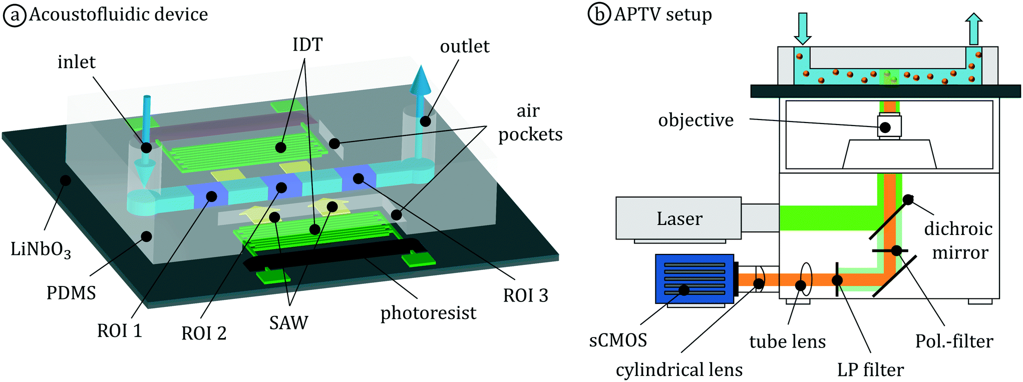Fig. 2 (a) Schematic illustration of the acoustofluidic device based on a 1D tweezer utilizing SAW. Flow measurements were conducted in three regions of interest (ROI 1–3). The directions of the counter propagating SAWs are indicated by yellow arrows. (b) Setup of the APTV system with the microchannel on top of a microscope. The paths of the laser light (green, λ_Laser = 532 nm) and the fluorescent light beam (orange, λ_Fluo = 607 nm) are highlighted accordingly.

Symmetrically to the microchannel, two IDTs consisting of a 5 nm adhesion layer of titanium and a 295 nm aluminum layer were deposited by electrode beam evaporation. In addition, a 385 nm thick layer of silicon dioxide (SiO₂) serves to protect the electrode structures from corrosion and mechanical damage. The width and spacing of the finger electrodes were varied in different chips, to investigate the effect of the wavelength on the acoustically excited flow in three steps from 20 μm to 150 μm. The aperture of the IDT AP was kept constant at 2 mm, while the number of finger electrodes was varied, in order to realize an impedance matching at 50 Ω.

The excitation of the SAW was performed with a defined electrical power by a PowerSAW generator (BelektroniG GmbH). The common resonance frequency was set based on the minima of the reflection factors S₁₁ and S₂₂ of both IDTs. A main flow was imposed with a syringe pump (neMESYS, cetoni GmbH), which fed the fluid with constant volume flow through metal cannulas into the microchannel. For a pulsation free fluid delivery, glass syringes (ILS Innovative Laborsysteme GmbH) with a volume of 100 μl as well as 250 μl were used.

For the entire investigation, three-dimensional flow measurements were performed using the astigmatism particle tracking velocimetry (APTV)⁵⁷ in three distinct regions of interest (ROI, see Fig. 2(a)). Here, we focus on the center (ROI 2), while the measurement results obtained in the outer parts (ROI 1 & ROI 3) of the acoustic excitation are discussed in Part II. The acoustofluidic platform was mounted on an inverted microscope (Axio Observer 7, Zeiss GmbH) with a Plan-Neofluar objective (M20×, NA = 0.4, Zeiss GmbH) (see Fig. 2(b)). Details about the optical arrangement of the APTV setup can be found in König et al. (2020).⁵⁸ In order to facilitate flow measurements, polystyrene particles containing a fluorescent dye (coumarin, excitation/emission at 530 nm/607 nm) were used. To illuminate these particles, a modulatable OPSL laser (λ_Laser = 532 nm, P_Laser,max = 8 W, tarm laser technologies tlt GmbH & Co. KG) was utilized, to enable measurements with a good signal-to-noise ratio (SNR). To avoid particle streaking, the illumination duration was adjusted in the respective parameter set using a function generator (Tektronix UK Ltd.).

Astigmatism particle tracking velocimetry is based on the determination of all three velocity components by tracking tracer particles with the highest possible flow fidelity. However, in acoustofluidics the particle motion is additionally affected by F_ARF (see eqn (8)). In order to keep the flow fidelity of the tracer particles high, two factors have been considered for the experiments. First, fluorescent polystyrene particles (PS-FluoRed, MicroParticles GmbH) with a radius of r = 0.57 μm or 0.225 μm were suspended in the fluid to reduce the influence of the acoustic radiation force (F_ARF ∝ r³, see eqn (8)), but still allowing reliable flow measurements with a sufficiently high SNR. Second, an aqueous glycerol solution (80% deionized water and 20% glycerol) was used as fluid to match the density between the particles and the fluid, which reduces the acoustic contrast factor ϕ and thus the influence of the acoustic radiation force (F_ARF ∝ ϕ⁵⁶) as well as sedimentation effects. The probability of particle agglomeration was reduced by the addition of 0.2% v/v surfactants (polysorbate 80, Biorigin).

Due to the limited optical access, both the image acquisition with an sCMOS camera (imager sCMOS, LaVision GmbH, 16 bit, 2560 × 2160 pixel) and the illumination were performed through the birefringent LiNbO₃ from the bottom side of the channel. To suppress double refraction a linear polarization filter⁴⁶ was inserted to the detection path within the microscope, see Fig. 2(b). In the optical path to the camera were also a dichroic mirror (DMLP567T, Thorlabs Inc) and a long pass filter (FELH0550, Thorlabs Inc) to separate reflected laser light from the fluorescent light of the particles. An additional cylindrical lens with a focal length of 250 mm, which was positioned approximately 40 mm in front of the camera, causes the particle images to appear elliptical and thus allows for the determination of the depth position (z) of the particles within the measurement volume by a calibration function.⁵⁹ The measurement volume extends over a length of 800 μm in the main flow direction (y), the entire channel width and approx. 45 μm in z-direction. However, in order to cover the entire channel height, the measurement volume was traversed through the whole height of the channel. The step sizes amounted to 10 μm or 15 μm for particle radii of 0.225 μm or 0.57 μm, respectively. At each position, 750 double images were acquired with a time interval Δt. These images were preprocessed by a background subtraction and applying a Gaussian filter with a kernel size of 5 × 5 pixels to smooth out image noise. Particle images were identified and segmented by a global threshold in the intensity level. Sub-pixel accuracy determination of particle positions in the (x,y) plane and lengths of semi-axes (ax,ay) was achieved by one-dimensional Gaussian fits in x and y-direction, respectively. Particle images with an Euclidean distance of less than 7.5 pixel to the calibration function in the (ax,ay) plane were considered as valid particle detections.⁶⁰ For particle tracking a simple nearest-neighbor algorithm was applied.⁶¹ With the estimated displacement vector d and the time interval Δt, the individual particle velocity vectors were determined by u = d/Δt. The randomly distributed vectors were then interpolated onto a regular grid using a Gaussian weighting based on the Euclidean distance to the center of a voxel. Velocity vectors whose components u_i with i = x,y,z differed by more than from the median within a voxel were excluded.

3.2 Numerical framework

To allow for a deeper insight into the physical mechanisms that drive the acoustically excited flow, numerical calculations were performed on the experimental parameter sets. With a systematic fitting of critical parameters based on the measured velocity data (see section 3.3), we obtain a validated numerical model that can reveal the first-order field quantities and thus the source terms of the stationary fluid motion. For this, the model initially solves the first-order eqn (1)–(3) numerically, which solution is subsequently used to calculate the second-order flow variables using the eqn (4)–(6). All simulations in this study were implemented in an Eulerian description of the quantities using the commercial software Comsol Multiphysics 5.6.⁶²

Since the flow in the center of the SAW field (ROI 2) is translationally invariant to a good approximation, we chose a two-dimensional model that comprised the analyzed system to the fluid domain in the channel cross-section with a height H and a width W (see Fig. S1, ESI†). This reduced approach showed good results in literature.^{38–41,68,73} In addition, low computational efforts enable parameter studies within reasonable time. Nevertheless, increased convergence to the measurements can be achieved by modeling not only the fluid domain, but also the PDMS channel^45,74 or the entire acoustic platform.^{43–45,75–78}

The longitudinal (dx) and transversal (dz) surface displacement at the channel bottom can be described for the case of two counter propagating SAWs as follows.

Here, k = 2π/λ_SAW describes the wavenumber, ω = 2πf the angular frequency, and  the displacement amplitude. In eqn (13), a phase shift of π/2 by multiplication with the imaginary unit i and a sign change were included to correctly capture the elliptical surface displacement.³⁸ Furthermore, the wave propagating to the left is phase-shifted by π to ensure that an anti-node is located in the center of the channel. The ratio of the displacement amplitudes in x and z direction ξ is based on the analytical solution of the Rayleigh wave⁶⁸ and amounts to 0.6746 in the used data set. The attenuation coefficient C_d of the SAW is theoretically determined by⁷⁹

Please note that the actual attenuation coefficient may differ due to inaccurate material properties and the influence of the SiO₂ layer on top of the substrate. The material properties implemented are listed in Table 1. Assuming a harmonic time dependence e^iωt, the surface displacement velocities u_x and u_z can be derived by differentiating the eqn (12) and (13) with respect to time t. These take the following form for an analysis in frequency space after removing the time dependence.^38,68

Table 1 Parameters and material properties at T = 25 °C used in the numerical calculations

Quantity	Symbol	Value
a Fitted to experimental data (see section 3.3). b Calculated as κ = 1/(ρfc^2f). c Value of pure water. d Calculated as Cp = 0.8 Cp,water + 0.2 Cp,glycerol with the specific heat capacity of water^70 and glycerol,^71 respectively. e Calculated with the heat capacity ratio of water.^41 f As provided by the manufacturer (Siegert Wafer GmbH). g Adapted from experimental values (cSAW = λSAWf). h As provided by the manufacturer (MicroParticles GmbH). i Calculated as κp = 3(1 − σp)/((1 + σp)ρpc^2p).^72
Fluid
(water (80%) – glycerol (20%) mixture)
Density^63	ρ f	1.05 g cm^−3
Speed of sound^a	c f	1576 m s^−1
Compressibility^b	κ	0.3834 GPa^−1
Shear viscosity^64	μ	1.5152 mPa s
Bulk viscosity^c^65	μ B	2.485 mPa s
Thermal expansion^66	α	4.04 × 10^−4 K^−1
Thermal conductivity^67	k th	0.525 W m^−1 K^−1
Heat capacity at const. pressure^d	C p	3821 J kg^−1 K^−1
Heat capacity at const. volume^e	C V	3779 J kg^−1 K^−1
Lithium niobate (LiNbO3)
Density^f	ρ S	4.64 g cm^−3
Speed of sound^g	c SAW	3860 m s^−1
Displacement ratio^68	ξ	0.6746
Polystyrene particles
Density^h	ρ p	1.05 g cm^−3
Speed of sound^69	c p	2350 m s^−1
Poisson's ratio^40	σ p	0.35
Compressibility^i	κ p	249 TPa^−1

---

Due to the high frequencies f of the SAW in the MHz range, the viscous boundary layer thickness δ varies between 48.6 nm and 133.7 nm within the parameter sets studied. Thus, to allow the fluid to follow the high-frequency tangential accelerations of the substrate surface without slip, high shear stresses τ are required in this small region.^80,81 For this reason, the no-slip boundary condition usually assumed at the channel bottom was replaced by a slip velocity considering the Navier slip length L_s according to u₁ = u_x + (L_s/μ)τ. For implementation, a stress boundary condition according to

was set at the channel bottom (z = 0). Here, n = (0,1)′ denotes the unit vector normal to the substrate surface. This more realistic boundary condition represents free-slip conditions for L_s → ∞ and the no-slip case for L_s → 0. The slip length L_s was obtained by fitting based on the measured velocity field as described in section 3.3. Due to the transversal displacement of the substrate surface, the fluid in the vicinity of the channel bottom is displaced vertically. To account for this, the fluid velocity normal to and at the substrate surface is prescribed by the transversal displacement velocity according to w₁|_z=0 = u_z.

To mimic the PDMS channel, impedance boundary conditions and a free-slip condition were implemented at the remaining channel boundaries. Due to the small mismatch between the impedance values of the fluid Z_f and the PDMS Z_PDMS, only a minor fraction of the incoming BAWs is reflected back into the fluid. Transmission of longitudinal waves from the PDMS into the fluid were neglected due to total reflection at the corresponding interface.⁴⁶ However, if these waves are previously reflected at the outside of the PDMS, transmission into the fluid is possible. In this case, as the path in the PDMS increases, the attenuation of the wave also increases significantly. As shown in Ni et al. 2019,⁴⁵ there are minor effects on the calculated flow patterns.

After the first-order thermodynamic quantities have been calculated with the predefined Thermoviscous Acoustics Interface, the solutions for u₁, p₁ and ρ₁ are used to estimate the steady flow with the Laminar Flow module. Following the model of Muller et al. (2012),⁵¹ the source term F in eqn (5) is implemented as a body force term and the right-hand side of eqn (4) as a mass source in a weak formulation. The fourth-order term ρ_f〈(u₂·∇)u₂〉_t was additionally retained in eqn (5). Due to the small influence on the flow field, the bulk viscosity was neglected in the second-order equations.⁵⁰ Dirichlet no-slip boundary conditions were set on the outer sides of the channel for the slow and steady streaming fluid.

Rectangular elements with refinement towards the channel edges were used to mesh the computational domain (see Fig. S1, ESI†). Based on a convergence study (see Fig. S2, ESI†) and considering the computational effort, the maximum element size in the bulk was set to 1.5 μm. The simulations were carried out on a high-performance computing cluster with Intel Xeon E5-2650 v4 processors (2.20 GHz) in parallel batch jobs on 12 cores.

3.3 Validation of the numerical model

One major problem for the simulation of the acoustically induced fluid flow originating from SAW is given by the materials used for the acoustofluidic setup. Their properties are mostly not well known and cover a wide range in literature. Therefore, the resulting flow field can significantly differ depending on the actual parameter set used. In order to validate the numerical model, the initial focus is on the adjustment of these critical material parameters. For this, a two-dimensional parameter sweep for the slip length L_s and the impedance of the PDMS channel Z_PDMS was performed separately for all configurations. For a quantitative comparison of the measured and calculated velocity of the suspended polystyrene particles based on the flow structures, a normalized 2D cross correlation was used. A detailed description on the comparison of both velocity fields can be found in the ESI.†

According to literature data,^82–91 the impedance of PDMS was varied in the range of 0.8 × 10⁶ Pa s m⁻¹ to 1.3 × 10⁶ Pa s m⁻¹. Responsible for the large variation are small deviations in the ratio between base and curing agent, the curing time and duration in the oven as well as aging processes that remained unknown. Since different microchannels were used during the experiments, it is necessary to adjust the impedance of the PDMS for all investigated parameter sets independently. For an wavelength of 90 μm and a channel height of 185 μm, Fig. S3 (ESI†) shows the correlation coefficient for different impedance values as a function of the slip length. The best match between numerical and experimental data for that case is obtained for Z_PDMS = 0.9 MPa s m⁻¹ and L_s = 1.5 μm, which is close to the free-slip case. The determined values for Z_PDMS and L_s are given in Table S1.†

In the next step, the sound velocity in the fluid was varied. Due to temperature influences and small deviations in the mixing ratio of water and glycerol, a range of 1565 m s⁻¹ to 1590 m s⁻¹ was investigated. This range has further been reported in literature.^92–98 Since the fluid remained unchanged between the measurements, this analysis was done only for the configuration using a wavelength of 90 μm and a channel height of 185 μm. The speed of sound was set to c_f = 1576 m s⁻¹.

The last important parameter for simulation is the displacement amplitude  which only influences the velocity amplitude, but has no influence on the structure of the flow in the investigated power range.⁴¹ The estimation of  with the supplied electrical power P_el is based on the following relationship.⁹⁹

Here AP = 2 mm denotes the aperture of the IDTs and F_N = 2.47 × 10¹⁵ W m⁻² a material dependent factor. The additionally implemented parameter k_η ∈ [0,1] indicates the amount of the electrical power to be considered for the calculation of the displacement amplitude. This includes losses due to reflections of the voltage signal during excitation of the SAW and attenuation of the SAW by the channel side walls, which vary for different experimental configurations. The normalized correlation coefficient R_num,exp is plotted in Fig. 4 for different configurations versus k_η. Overall, values greater than 0.85 were always obtained in the correlation with P_el = 30 mW, which indicates a good agreement between experiment and simulation. The results of the parameter fitting are discussed more detailed in the following section.

4 Results and discussion

4.1 Acoustically induced streaming pattern

The experimentally analyzed parameter sets include systematic variations in the channel height, the wavelength of the SAW and the applied electrical power. The latter was varied in the range of P_el ∈ [10,30] mW. However, P_el only affects the magnitude of the fluid velocity but not the streaming pattern. Therefore, main focus is pointed to the channel height and wavelength of the SAW. Fig. 3 shows an overview of the time-averaged absolute velocity fields transverse to the main flow in the center of the acoustic excitation at wavelengths of 20 μm, 90 μm and 150 μm as well as channel heights of about 85 μm, 185 μm and 530 μm. Since the flow is translationally invariant along the longitudinal channel axis (y), the velocity fields were obtained by averaging all determined velocity vectors over the entire length (800 μm) of the measurement volume. An impact of the flow rate on the transverse components u and w can also be neglected. Therefore, the volume flow rate was adjusted between 0.15 μl min⁻¹ and 4 μl min⁻¹ to optimize the time interval Δt between image captures, yielding reliable velocity measurements with low uncertainty. The experimental results illustrate a clear dependence of the flow structures on the wavelength of the SAW and the channel height, which will be discussed in detail in sections 4.2 and 4.3, respectively. Regardless of the actual configuration, a symmetrical streaming pattern occurs. Especially at small wavelengths and large channel heights, large vortex structures develop that extend symmetrically from the lateral channel walls over the entire channel cross-section (see Fig. 3). However, as the wavelength increases or channel height decreases, a periodic flow structure develops in the center of the channel. For the highest wavelength and lowest channel height, the particle motion is strongly affected by the standing pressure field and the acoustic radiation force, which will cause areas with particle depletion as well as agglomerations at pressure nodes. In order to keep the influence of F_ARF on the particle motion low, smaller tracer particles with a radius of r = 0.225 μm were used for reliable flow measurements in the configurations with λ_SAW = 150 μm and λ_SAW = 90 μm (H = 85 μm and H = 185 μm) (see section 3.1). The few white areas close to the channel walls indicate regions where it was not possible to determine particle trajectories and thus no measured data exists.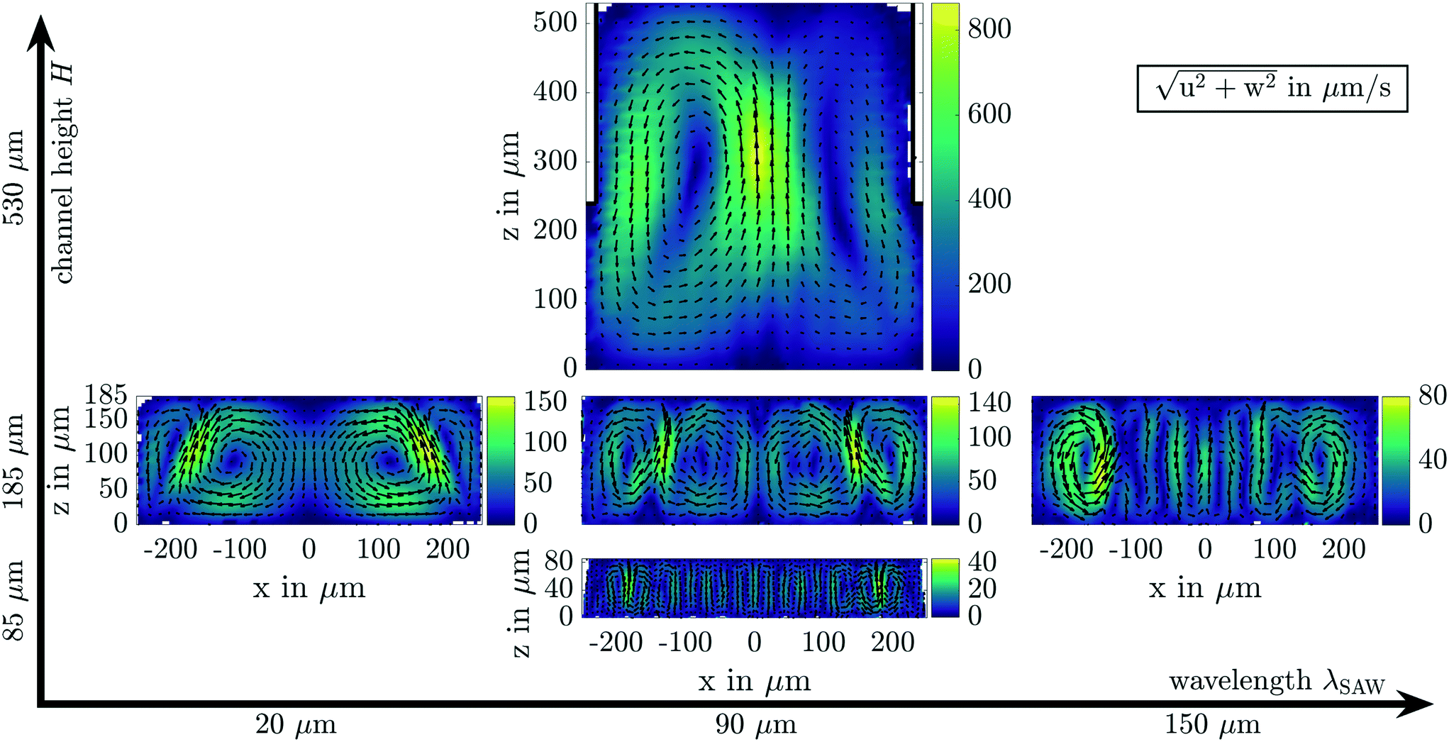

Fig. 3 Time-averaged absolute velocity fields transverse to the main flow for different parameter sets (varying wavelength in the horizontal direction and channel height in the vertical direction) obtained from experimental studies. The investigated wavelengths range from 20 μm over 90 μm up to 150 μm, while the channel height was varied in the steps 85 μm, 185 μm and 530 μm.

Furthermore, asymmetries within the velocity fields with respect to the z-axis can be attributed to deviations in the attenuation of the SAW by the channel side walls, the power coupling of the two IDTs as well as the phasing of the counter propagating SAWs. To interpolate the randomly distributed velocity vectors onto a regular grid, quadratic voxels with an edge length of 15 μm (H = 530 μm), 10 μm (H = 185 μm), and 5 μm (H = 85 μm) were used with an overlap of 50%. For each measurement, the mean number of individual velocity vectors in each voxel was sufficiently large for reliable flow measurements.

4.2 Influence of the wavelength

To discuss the influence of the wavelength on the structure and velocity of the acoustically induced fluid flow, the experimental and numerical results are visualized by streamlines in Fig. 5. Based on this qualitative comparison, a strong similarity between experiment and simulation is evident and confirms the high correlation coefficient (Fig. 4). Furthermore, Fig. 5 illustrate that the measured particle velocity is close to the calculated flow velocity and thus the measures taken in section 3.1 to reduce the influence of F_ARF on the resulting particle motion were effective.

Fig. 4 Correlation coefficient R_num,exp between numerical and experimental particle velocities as a function of the coupling factor k_η for different wavelengths λ_SAW and channel heights H. the supplied electrical power is constant at P_el = 30 mW.

Fig. 5 Time-averaged absolute velocity field transverse to the main flow for wavelengths of 20 μm (a), 90 μm (b), and 150 μm (c). The positions of the vortex centers are indicated by red asterisks. Experimental results are shown on the left half and numerical results on the right half.

The qualitative comparison of the symmetrical flow fields shows a transition from large to small vortex structures with increasing wavelength. While large vortex structures extend over several pressure nodes for low wavelengths (Fig. 5(a)), a periodic flow structure (Fig. 5(c)) prescribed by the standing pressure field evolves for large wavelengths. This behavior can be explained by the scaling of the attenuation coefficient C_d ∝ λ⁻¹_SAW with wavelength. The greater attenuation of the counter propagating SAWs at small wavelengths results in varying amplitudes of the surface displacements along the channel width. For λ_SAW = 20 μm (C_d = 4658 m⁻¹), significant discrepancies between the amplitudes of the counter propagating SAWs are present over large parts of the channel, while these are limited to a region near the channel side walls in the case of λ_SAW = 150 μm (C_d = 615.6 m⁻¹). These discrepancies manifest themselves in traveling wave components and provide the energy to form the acoustically excited flow by means of viscous damping. Consequently, characteristic vortex structures form under consideration of mass conservation as Eckart flow only close to the side walls of the channel in the latter configuration. In the center of the channel, however, the standing wave field dominates, which results from the superposition of the counter propagating SAWs with almost the same amplitude.

The weaker attenuation of the SAW at larger wavelengths indicates that a smaller fraction of the energy transported by the wave is radiated into the liquid. This effect is enhanced by the lower viscous damping of the BAW in the fluid, which is mainly transmitted into the PDMS at the channel ceiling. As a result, a decreasing fluid velocity is observable. Another aspect to drive the acoustically induced flow consists in pressure gradients in the first-order fields,³⁸ which are more pronounced with decreasing wavelength of the SAW (see Fig. S5, ESI†). Especially the formation of anechoic corners^17,100 with lower pressure amplitudes at the upper channel margin supports the prior assumptions regarding the structure of the flow. In the fluid motion at λ_SAW = 20 μm, which is strongly influenced by traveling wave components, the angle between the outer and inner vortex pairs can be determined to be about 24.2°. This is close to the theoretical Rayleigh angle of θ_Fluid = 24.1° and thus confirms the flow characteristic, which is similar to that excited by a pure traveling wave, as measured by Kiebert et al. (2017).⁴⁶ This streaming angle decreases with rising wavelength, while the vortex centers of the outer vortices are shifted towards the center of the channel. In addition, the larger the wavelength the higher the number of vortex pairs over the entire cross-section of the microchannel. Independently of the actual wavelength, the highest fluid velocity occurs at the inner edge of the outer vortices in all investigated configurations.

The high similarity between numerical and experimental results is further revealed by the vertical velocity component, which is plotted along a horizontal line at half channel height in Fig. 6(a). When comparing the velocity curves for different wavelengths of the SAW, the increasingly periodic fluid flow becomes apparent when magnify the wavelength. Especially close to the channel center, a periodicity of 45.9 μm can be determined, which agrees well with the periodicity of the pressure field prescribed by two counter propagating SAWs with 90 μm wavelength (see also Fig. S6, ESI†). Although two widely extended vortex pairs form for λ_SAW = 90 μm in Fig. 5, the influence of the standing wave field is evident based on the velocity curves in Fig. 6(a).

Fig. 6 (a) Velocity component w or w₂ for experimental (left) and numerical results (right), respectively, along a horizontal line at z = H/2 for different wavelengths. Kinetic energy density (b) and kinetic efficiency (c) from measurements (Δ) and simulations (°) as a function of the wavelength λ_SAW for different electrical power levels P_el. Thereby P_el = (10.09 ± 0.26) mW is assigned as 10 mW, (20.28 ± 0.63) mW as 20 mW and (29.72 ± 0.13) mW as 30 mW for the experimental data. The error bars indicate a confidence interval of 95%.

After analyzing the structure of the flow, the focus will be on an energetic consideration in the following. For this purpose, the mean kinetic energy density,

of the acoustically driven fluid flow in the x–z-plane is plotted in Fig. 6(b) for different wavelengths and electrical power levels for the microchannel with 185 μm in height. As expected, the kinetic energy density increases with increasing supplied power. Overall, a mean difference between the experiments and numerical approximations of 8.81% identify a reasonable agreement. Furthermore, the larger the wavelength the lower e_kin, which is in accordance with the theoretical attenuation of acoustic waves according to eqn (14) and Stokes' law of sound attenuation. Beside those basic dependencies, the deviating coupling factors (Fig. 4) must also be taken into account, which shrink with decreasing wavelength and thus indicate increasing losses. The primary reason for the rising losses is the stronger attenuation of the SAW at the channel side walls. This is reflected in a significant decrease of the coupling factor between the results with λ_SAW = 90 μm and λ_SAW = 20 μm, which in turn affects the kinetic energy of the fluid motion. A progressive rise of power loss at the channel side walls with decreasing wavelength was demonstrated by Winkler et al. (2016)¹⁰¹ and further confirmed here by estimating the SAW attenuation based on the scattering parameter |S₁₂ | (see Fig. S7, ESI†).

Based on the kinetic energy measured, the kinetic efficiency can be determined with η_kin = e_kinHWc_SAW/(P_elλ_SAW). As illustrated in Fig. 6(c), the η_kin decreases monotonically with the SAW wavelength, which complies with the fundamental dependencies on sound attenuation mentioned above. Using a wavelength of the SAW close to the channel height of about 185 μm, the kinetic efficiency drops to about 2.4 × 10⁻⁸. Regardless of the actual values, the results obtained confirm an efficiency of fluid flow actuation in the range of 10⁻⁸ to 10⁻⁶, as also estimated in literature so far.¹⁰²

Due to the close match between simulation and experiment, it is reasonable to calculate the first-order field quantities and extend the energetic consideration to the average acoustic energy density E_ac according to eqn (7). The results are depicted in Fig. 7. Even though the acoustic energy density turns out to be low in the investigated power range, the rising curves show that more energy is contained in the first-order acoustic fields with increasing wavelength. With respect to the resulting acoustic radiation force, this results in two opposite phenomena. First, the F_ARF scales inversely proportional with λ_SAW (F_ARF ∝ λ⁻¹_SAW), while second, the increase in E_ac is propagated proportionally in the F_ARF ∝ E_ac. Consequently, this scaling is crucial to determine the critical particle diameter^36,103 above which the particle motion is dominated by F_ARF.

Fig. 7 Acoustic energy density E_ac as a function of the wavelength λ_SAW obtained by numerical simulations for different electrical power levels.

In the context of a particle separation, the analysis of the superimposed flow leads to advantages for SAW systems with small excitation frequencies or large wavelengths from the following aspects:

• Periodic flows spatially limit the hydrodynamic displacement of small particles, which motion is not dominated by F_ARF, especially in the region of the center of the channel.

• The fraction of the supplied energy that is converted into kinetic energy decreases with λ_SAW, causing particle trajectories to be more influenced by F_ARF instead of Stokes' drag.

4.3 Influence of the channel height

Besides the wavelength of the SAW, also the channel geometry has a strong influence on the acoustically excited flow field. In this study, the focus is on a rectangular channel cross-section, which is predominantly used in microfluidics. Following the numerical results of Devendran et al. (2016),³⁸ larger discrepancies in the SAW amplitude distribution of standing SAW across the channel width are expected with increasing channel width, which cause traveling wave components and stronger vortex structures close to the side walls of the channel. Since these are undesirable in separation systems with tilted IDTs, small channel widths are preferable from a hydrodynamic point of view. However, a conflict arises in terms of the maximum lateral displacement of particle fractions, which is limited by the channel width and thus influences the separation efficiency.

Based on experimental and numerical investigations, the effect of the channel height will be further examined in the following. The channel width was kept constant at (500 ± 10) μm and the height was varied in the interval H ∈ [85,185,530] μm. Deviations from the rectangular channel cross-section occur only in the largest channel, whose width reduces to about 460 μm for z ≥ 240 μm. This is caused by the milling process of the associated aluminum master mold, yielding a step in the side channel wall. A corresponding adjustment of the geometry was considered in the numerical model. Furthermore, a symmetrical boundary condition was set for the first and second-order field quantities in the center of the channel (x = 0). Calculations were only performed for half the computational domain (x ≥ 0) in order to meet hardware limitations. To find the slip length for the best matching result, a separate cross correlation was performed with only considering the region near the channel bottom (z < 30 μm), since small vortices, that are characteristic for the no-slip boundary condition (see Fig. S4, ESI†), would otherwise be underestimated within the large channel height. The normalized correlation coefficient was subsequently multiplied by that of the cross correlation for the global velocity field. The resulting coefficient was used as an indicator for the best match between experiment and simulation. By considering the correlation coefficients (>0.85) in Fig. 4, a good agreement between numerical (right) and experimental (left) solution can be stated in Fig. 8.

Fig. 8 Time-averaged absolute velocity field transverse to the main flow for channel heights of 530 μm (a), 185 μm (b), and 85 μm (c). The positions of the vortex centers are indicated by red asterisks. In the divided plot, experimental results are shown on the left half and numerical results on the right half, respectively. The excitation frequency is constant at 42.88 MHz.

With a common wavelength of 90 μm, a transition from broadly extended vortex structures to periodic flow patterns is visible with decreasing channel height, as shown in Fig. 8. A comparable behavior of the flow structure has already been observed for increasing wavelengths at a fixed channel height (see Fig. 5). The fluid flow occurs in the largest channel as a single vortex pair with a global velocity maximum in the center of the channel (x = 0), symmetrical to the z-axis. According to the flow field depicted in Fig. 8(a), no influence of the standing wave field is visible. However, very small periodic fluctuations of the velocity component w and w₂ exist. Details can be found in supplementary information, Fig. S8.† By reducing the channel height, the number of vortex pairs increases, with two separate velocity maxima forming at the inner edge of each outer vortex. This development originates in the radiation characteristic of the BAW at a Rayleigh angle of θ_Fluid = 24.1°. A decisive factor for the lateral extent of these vortices is the distance W* = H tan(θ_Fluid) from the side walls of the channel, covered by the BAW in the x-direction before reaching the channel ceiling. With W* < λ_SAW/2 follows H_crit < λ_SAW/(2 tan(θ_Fluid)) as a critical channel height, which should not be exceeded to suppress large streaming vortices, that extend across several pressure nodes. In order to limit the influence of traveling wave components, the ratio of the amplitude of the emanating SAW to the amplitude of the counter propagating SAW close to the channel side wall needs to be limited. Based on numerical calculations, this ratio should be larger than 0.6, which leads to a definition of a critical channel width of W_crit < −ln(0.6)/C_d from eqn (14). Accordingly designed channel geometries lead to a periodic flow pattern with limited extent of vortices evolving close to the channel side walls. This critical channel width and height was fulfilled for the experimental configuration corresponding to the flow field depicted in Fig. 8(c). For further examples, the interested reader is referred to Fig. S9 (ESI†).

Regarding the kinetic energy density it applies: the larger the channel height compared to the wavelength of the BAW the higher the kinetic energy density. This behavior corresponds to the influence of the frequency, at which e_kin increases with decreasing wavelength of the BAW at a constant channel height. Overall, the channel height has a stronger influence on the acoustically induced fluid flow than the wavelength. Thus, over the entire power range, the lowest and highest mean kinetic energy densities were obtained at the smallest (H = 85 μm) and largest channel height (H = 530 μm), respectively. Furthermore, the damping of the BAW give rise to gradients in the amplitudes of the first-order fields in z-direction, which lead to a decreasing average acoustic energy density when increasing the channel height. Although this influence is significantly weaker than the impact of the wavelength on E_ac, the resulting acoustic radiation force (F_ARF ∝ E_ac) decreases on average as well. Hence, the ratio between channel height and wavelength is of importance, which should be small for separation systems making use of F_ARF.

For those systems, the following conclusions can be drawn for a decreasing channel height:

• Weaker vortex structures with smaller lateral extent offer advantages for separating small particles whose motion is not dominated by the acoustic radiation force.

• An increase in the mean acoustic energy density results in a stronger F_ARF, which allows operation with lower electrical power.

4.4 Electrical power

In the third dimension of the investigated parameter set, the applied electric power P_el was varied in three steps from approx. 10 mW to about 30 mW. In contrast to the SAW wavelength and channel height, P_el affects the fluid velocity but not the flow pattern. This assumption can be exemplified in both experimental and numerical data by the horizontal profile of the vertical velocity component w and w₂, respectively, in Fig. 9. Here, the channel height amounts to 185 μm and the excitation frequency is 42.88 MHz, which corresponds to a wavelength of about 90 μm. In the comparison among the three curves of different electrical power level, the shape remains unchanged, while an increase of the absolute fluid velocity with rising P_el can be observed throughout the whole channel width.

Fig. 9 Profiles of the velocity component w and w₂ along a horizontal line at z = H/2 for different electrical power levels. Experimental data is presented in the left half, while numerical results are shown in the right half. The electrical power was truncated to 10 mW, 20 mW, and 30 mW in the simulations. The channel height is constant at H = 185 μm and the wavelength amounts to λ_SAW = 90 μm.

To quantify the scaling of the associated mean kinetic energy density with the electrical power, e_kin(P_el) is plotted in Fig. 10(a). The different curves represent the considered parameter sets of wavelength and channel height and extend across more than four orders of magnitude. In all parameter sets, monotonically ascending curves show a progressive, nonlinear behavior when increasing P_el for both the experimentally and numerically generated results. However, deviating curves are conceivable for larger electrical powers of up to 9 W,³⁴ which are used in separation systems with relatively high throughput. In such cases, increased dissipation effects in the fluid, attenuation losses of the SAW through the channel wall and the effect of secondary Bjerknes forces due to wave scattering by the particles⁴⁷ should be considered.

Fig. 10 Average kinetic energy density (a) obtained from measurements (colored symbols) and simulations (black symbols) as a function of the electrical power for various combination of the channel height H and the wavelength λ_SAW. The error bars indicate a confidence interval of 95%. The corresponding acoustic energy density was determined numerically based on eqn (7) and is plotted in subplot (b) versus the electrical power P_el.

Based on simulations, the mean acoustic energy density E_ac is shown in Fig. 10(b) as a function of the electrical power. Here, E_ac grows proportionally to the imposed electrical power in the investigated range for all given parameter sets. This is consistent with the scaling of E_ac ∝ U²_pp ∝ P_el given by Bruus et al. 2012,¹⁰³ where U_pp is the applied peak to peak voltage. However, for a larger power range, a dependence of the coupling factor k_η, which was kept constant in the respective parameter set, on the electrical power may not be negligible. This in turn affects the scaling of the average acoustic energy density. At this point, subsequent studies are conceivable, where measurements at higher electrical power levels or more sophisticated numerical models, that consider the entire acoustofluidic platform, are used.

4.5 Acoustophoretic particle motion

The motion of suspended microparticles in a standing acoustic wave field is primarily determined by the acoustic radiation force F_ARF and the Stokes' drag due to the fluid flow. In SAW-based separation systems, situations are commonly intended where F_ARF acts as the dominant force and focuses particles with an acoustic contrast factor ϕ > 0 at pressure nodes. The spatial distribution of |F_ARF| reveals annular structures with force vectors always pointing away from the antinodes (see Fig. S10, ESI†). Hence, stable equilibria form only at the pressure nodes, although |F_ARF| decays to zero also at the antinodes. This force field is linearly superimposed on the Stokes' drag for a fixed particle (u_p = 0) inside the acoustically induced fluid flow according to F_Drag = 6πμru₂. The relative influence of both forces on the particle motion can be determined by the force coefficient |F_ARF|/|F_Drag|. In Fig. 11, the spatial distribution of the force coefficient is depicted for a SAW wavelength of 90 μm and a channel height of 185 μm across the channel cross-section. Besides the previously discussed parameters, |F_ARF|/|F_Drag| is additionally influenced by the particle radius r, which was set to 0.69 μm in the selected example.

Fig. 11 Spatial distribution of the force coefficient |F_ARF|/|F_Drag| for a wavelength of 90 μm, a channel height of 185 μm and an electrical power of 20 mW. The color scale is capped at 1 to highlight yellow areas, where |F_ARF| dominates over the Stokes' drag due to the fluid flow. The particle radius amounts to r = 0.69 μm, resulting in a mean force coefficient of ψ ≈ 1.

A spatial dependency of the force coefficient is revealed, in which values greater than one indicate a particle motion dominated by F_ARF near the channel ceiling and floor. This is confirmed by experiments in which particles were initially focused at the pressure nodes in these regions of the microchannel. Furthermore, the influence of the attenuation of the counter propagating SAWs is reflected by greater values in the channel center (−100 μm ≤ x ≤ 100 μm), where the fluid flow is dominated by the standing wave field and F_Drag loses impact compared to F_ARF. In contrast, traveling wave components provide the drive for strong vortices near the channel side walls, which mainly determine the particle motion, as can be recognized by a lower force coefficient.

A quantitative evaluation of the force ratio for different configurations regarding the wavelength, channel height, and particle radius is based on the mean force coefficient ψ = 〈|F_ARF|/|F_D|〉_A, that is obtained by averaging over the entire channel cross-section A. The scaling of the Stokes' drag (F_Drag ∝ r) and the acoustic radiation force (F_ARF ∝ r³) with the particle radius yields a quadratic dependence ψ ∝ r², which can be confirmed by the numerical results shown in Fig. 12. Moreover, an increase of ψ with the wavelength of the SAW λ_SAW is revealed, which is caused by the rising mean acoustic energy density (F_ARF ∝ E_ac) and the decreasing mean kinetic energy density (F_Drag ∝ e^1/2_kin), as outlined in section 4.2. This development thus compensates the direct inverse relation of F_ARF to the wavelength (F_ARF ∝ λ⁻¹_SAW).

Fig. 12 Mean force coefficient ψ as a function of particle radius r for different configurations with the wavelength of the SAW λ_SAW and channel height H. In the inset, the course up to the critical value ψ_crit = 1 is depicted for particle radii below 1 μm. The numerical results were connected by quadratic regressions.

However, the mean kinetic energy density increases with rising channel height, while the mean acoustic energy density decreases. Consequently, the particle motion is found to be stronger affected by the fluid flow with increasing channel height, which is reflected in lower values of ψ. The inset in Fig. 12 further shows the curves of ψ for particle radii r ≤ 1 μm up to a critical mean force coefficient of ψ_crit = 1, for which the effects of F_ARF and F_Drag compensate on average. Using ψ_crit, a critical particle radius r_crit can be defined below which the motion of the suspended particles is dominated by the SAW induced flow. The scaling of ψ ∝ E_acr²/(λ_SAWe^1/2_kin) leads to r_crit ∝ (λ_SAWe^1/2_kin/E_ac)^1/2 and thus a decrease of r_crit for an increasing wavelength or decreasing channel height. Throughout the experimental configurations, flow-dominated situations with ψ < 0.3 were maintained, which allowed a high flow fidelity of tracer particles with radii r ≪ r_crit and thus conclusions on the actual fluid flow.

Nevertheless, if a particle separation is to be achieved by the influence of F_ARF in SAW-based devices, the strong spatial dependence of |F_ARF|/|F_Drag| must be considered, because particle motion being dominated by F_ARF in less than 28% of the channel cross-section even for ψ = 1. Concerning particle separation systems, the following aspects can be concluded.

• The interplay of increasing E_ac and decreasing e_kin with rising wavelength compensate the scaling of F_ARF ∝ λ⁻¹_SAW for the particle motion and must be considered when determining a critical particle radius r_crit.

• The motion of particles with a radius smaller than r_crit is significantly affected by the SAW-induced flow.

• Shallow microchannels facilitate influencing particle trajectories by F_ARF.

5 Conclusion

Experimental three-dimensional, three component (3D3C) velocity measurements with astigmatism particle tracking velocimetry (APTV) and numerical simulations on the acoustically excited flow in the center of a standing surface acoustic wave (SAW) were performed. Against the background of a selective particle separation, an acoustic tweezer setup employing two counter propagating SAWs superimposed within a straight microchannel was investigated in detail. In this system, multiple pressure nodes along the channel width form, as typical in the application of high-frequency SAW-based separation systems. To determine crucial factors that affect the structure and scaling of the acoustically induced fluid flow, the wavelength of the SAW, channel height and electrical power were systematically varied. In this way, an influence on the flow pattern could be demonstrated for the former two, while the applied electrical power only affects the fluid velocity in the investigated range. A transition from vortex pairs that extend far across the channel cross-section to a periodic flow pattern can be observed with increasing wavelength. In association with the decreasing attenuation of the counter propagating SAWs, the periodic flow pattern occurs especially in the center of the channel. A similar characteristic of the fluid flow can be achieved with decreasing channel height, for which the decreasing traveling length and attenuation of the radiated bulk acoustic wave (BAW) in the fluid are causal. In both cases, the maximum flow velocity decreases. From a hydrodynamic point of view, there are thus advantages for the design of separation systems, particularly if very tiny particles need to be separated, which are less influenced by the acoustic radiation force (F_ARF). Based on the results, a critical channel height H_crit < λ_SAW/(2 tan(θ_Fluid)) and width W_crit < −ln(0.6)/C_d were derived, which should not be exceeded to suppress widely extended vortex structures.

Furthermore, a numerical model was developed in which the longitudinal displacement of the SAW was considered by a slip boundary condition at the substrate-fluid interface. In this model, critical parameters like the Navier slip length, the acoustic impedance of PDMS and the displacement amplitude were systematically adjusted based on the experimental data. With this approach, a very good agreement with the experimental velocity data was obtained, indicated by a correlation coefficient of R_exp,num > 0.85 for all experimentally investigated configurations. With the validated numerical model, further reliable studies can be performed without experimental limitations, also extending the insights to an energetic consideration based on the first- and second-order fields. Decreasing mean kinetic energy densities e_kin for increasing wavelengths could be confirmed in both experimental and numerical results. At the same time, the mean acoustic energy density E_ac increases due to lower attenuation losses of the SAW, thus providing advantages for particle separation in acoustic devices due to a higher influence of standing wave field components compared to traveling components. The proportional increase of F_ARF with E_ac needs to be considered, which counteracts the inverse scaling with the wavelength (F_ARF ∝ λ⁻¹_SAW). These fundamental dependencies found causes an optimization issue in the development of separation systems. Furthermore, the mean kinetic energy density drops for decreasing channel heights, while the mean acoustic energy density increases. Therefore, as similar for an increasing wavelength, the acoustically induced flow is suppressed while the influence of the F_ARF on the resulting particle motion increases with decreasing channel height. Hence, shallow microchannels and large wavelengths are advantageous for particle separation.

Besides these findings, a validated numerical model that captures the characteristics of the acoustically induced flow with a reasonable computational effort was developed. Based on our numerical model and the experimental data obtained, we highly encourage scientists to compare their numerical models. The experimental data can be found on https://github.com/sesa1504/AS_in_sSAW. A possible direction of subsequent studies is to investigate the influence of different channel materials, in which more complex wave superpositions can be captured experimentally or by numerical models that consider the entire acoustofluidic platform. To further extend the gained insights on acoustically driven flows, Part II of this study discusses the complex, three-dimensional vortex structures in the outer regions of the acoustic wave field, which needs to be considered for particle separation systems as well.

Author contributions

Sebastian Sachs: conceptualization, formal analysis, investigation, methodology, software, validation, visualization, writing – original draft. Mostafa Baloochi: software, validation. Christian Cierpka: project administration, resources, supervision, writing – review & editing. Jörg König: conceptualization, project administration, resources, supervision, writing – review & editing.

Conflicts of interest

There are no conflicts to declare.

Acknowledgements

The authors thank the German research foundation (DFG) for financial support under grant number CI 185/6-1 and within the priority program SPP2045 “MehrDimPart” (CI 185/8-1). Furthermore, we are grateful to M.Sc. Christian Koppka from TU Ilmenau, Center of Micro- and Nanotechnologies (ZMN) (DFG RIsources reference: RI_00009), a DFG-funded core facility (Grant No. MU 3171/2-1 + 6-1, SCHA 632/19-1 + 27-1, HO 2284/4-1 + 12-1), who helped in the preparation of the samples.

Notes and references

1. P. Sajeesh and A. K. Sen, Microfluid. Nanofluid., 2014, 17, 1–52.
2. M. Li, W. H. Li, J. Zhang, G. Alici and W. Wen, J. Phys. D: Appl. Phys., 2014, 47, 063001.
3. S. Patel, S. Qian and X. Xuan, Electrophoresis, 2013, 34, 961–968.
4. M. Ahmad, A. Bozkurt and O. Farhanieh, World J. Eng., 2019, 16, 823–838.
5. G. Zhu and N.-T. Nguyen, Micro Nanosyst., 2010, 2, 202–216.
6. A. Volpe, C. Gaudiuso and A. Ancona, Micromachines, 2019, 10, 594.
7. D. R. Gossett, W. M. Weaver, A. J. Mach, S. C. Hur, H. T. K. Tse, W. Lee, H. Amini and D. Di Carlo, Anal. Bioanal. Chem., 2010, 397, 3249–3267.
8. J. Zhang, S. Yan, R. Sluyter, W. Li, G. Alici and N.-T. Nguyen, Sci. Rep., 2014, 4, 4527.
9. M. Yamada, M. Nakashima and M. Seki, Anal. Chem., 2004, 76, 5465–5471.
10. S. Blahout, S. R. Reinecke, H. Tabaei Kazerooni, H. Kruggel-Emden and J. Hussong, Microfluid. Nanofluid., 2020, 24, 22.
11. J. McGrath, M. Jimenez and H. Bridle, Lab Chip, 2014, 14, 4139–4158.
12. T. A. Crowley and V. Pizziconi, Lab Chip, 2005, 5, 922–929.
13. M. Bayareh, Chem. Eng. Process., 2020, 153, 107984.
14. M. Wu, A. Ozcelik, J. Rufo, Z. Wang, R. Fang and T. Jun Huang, Microsyst. Nanoeng., 2019, 5, 32.
15. X. Ding, P. Li, S.-C. S. Lin, Z. S. Stratton, N. Nama, F. Guo, D. Slotcavage, X. Mao, J. Shi, F. Costanzo and T. J. Huang, Lab Chip, 2013, 13, 3626–3649.
16. Y. Gao, M. Wu, Y. Lin and J. Xu, Micromachines, 2020, 11, 921.
17. G. Destgeer, B. H. Ha, J. Park, J. H. Jung, A. Alazzam and H. J. Sung, Anal. Chem., 2015, 87, 4627–4632.
18. D. J. Collins, A. Neild and Y. Ai, Lab Chip, 2016, 16, 471–479.
19. J. Behrens, S. Langelier, A. R. Rezk, G. Lindner, L. Y. Yeo and J. R. Friend, Lab Chip, 2015, 15, 43–46.
20. J. Shi, H. Huang, Z. Stratton, Y. Huang and T. J. Huang, Lab Chip, 2009, 9, 3354–3359.
21. X. Ding, Z. Peng, S.-C. S. Lin, M. Geri, S. Li, P. Li, Y. Chen, M. Dao, S. Suresh and T. J. Huang, Proc. Natl. Acad. Sci. U. S. A., 2014, 111, 12992–12997.
22. G. Liu, F. He, X. Li, H. Zhao, Y. Zhang, Z. Li and Z. Yang, Microfluid. Nanofluid., 2019, 23, 23.
23. M. C. Jo and R. Guldiken, Sens. Actuators, A, 2012, 187, 22–28.
24. S. Gupta, D. L. Feke and I. Manas-Zloczower, Chem. Eng. Sci., 1995, 50, 3275–3284.
25. P. Li, J. Zhong, N. Liu, X. Lu, M. Liang and Y. Ai, Sens. Actuators, B, 2021, 344, 130203.
26. G. Destgeer, B. H. Ha, J. H. Jung and H. J. Sung, Lab Chip, 2014, 14, 4665–4672.
27. H. Ahmed, G. Destgeer, J. Park, M. Afzal and H. J. Sung, Anal. Chem., 2018, 90, 8546–8552.
28. T. Laurell, F. Petersson and A. Nilsson, Chem. Soc. Rev., 2007, 36, 492–506.
29. S. Zhao, M. Wu, S. Yang, Y. Wu, Y. Gu, C. Chen, J. Ye, Z. Xie, Z. Tian, H. Bachman, P.-H. Huang, J. Xia, P. Zhang, H. Zhang and T. J. Huang, Lab Chip, 2020, 20, 1298–1308.
30. M. Wu, P.-H. Huang, R. Zhang, Z. Mao, C. Chen, G. Kemeny, P. Li, A. V. Lee, R. Gyanchandani, A. J. Armstrong, M. Dao, S. Suresh and T. J. Huang, Small, 2018, 14, e1801131.
31. J. Nam, Y. Lee and S. Shin, Microfluid. Nanofluid., 2011, 11, 317–326.
32. C. Richard, A. Fakhfouri, M. Colditz, F. Striggow, R. Kronstein-Wiedemann, T. Tonn, M. Medina-Sánchez, O. G. Schmidt, T. Gemming and A. Winkler, Lab Chip, 2019, 19, 4043–4051.
33. P. Dow, K. Kotz, S. Gruszka, J. Holder and J. Fiering, Lab Chip, 2018, 18, 923–932.
34. P. Li, Z. Mao, Z. Peng, L. Zhou, Y. Chen, P.-H. Huang, C. I. Truica, J. J. Drabick, W. S. El-Deiry, M. Dao, S. Suresh and T. J. Huang, Proc. Natl. Acad. Sci. U. S. A., 2015, 112, 4970–4975.
35. M. Wu, Z. Mao, K. Chen, H. Bachman, Y. Chen, J. Rufo, L. Ren, P. Li, L. Wang and T. J. Huang, Adv. Funct. Mater., 2017, 27, 1606039.
36. R. Barnkob, P. Augustsson, T. Laurell and H. Bruus, Phys. Rev. E: Stat., Nonlinear, Soft Matter Phys., 2012, 86, 056307.
37. P. Sehgal and B. J. Kirby, Anal. Chem., 2017, 89, 12192–12200.
38. C. Devendran, T. Albrecht, J. Brenker, T. Alan and A. Neild, Lab Chip, 2016, 16, 3756–3766.
39. P. K. Das, A. D. Snider and V. R. Bhethanabotla, Phys. Fluids, 2019, 31, 106106.
40. N. Nama, R. Barnkob, Z. Mao, C. J. Kähler, F. Costanzo and T. J. Huang, Lab Chip, 2015, 15, 2700–2709.
41. R. Barnkob, N. Nama, L. Ren, T. J. Huang, F. Costanzo and C. J. Kähler, Phys. Rev. Appl., 2018, 9, 014027.
42. W. Qiu, J. H. Joergensen, E. Corato, H. Bruus and P. Augustsson, Phys. Rev. Lett., 2021, 127, 064501.
43. J.-C. Hsu and C.-L. Chao, J. Appl. Phys., 2020, 128, 124502.
44. W. N. Bodé, L. Jiang, T. Laurell and H. Bruus, Micromachines, 2020, 11, 292.
45. Z. Ni, C. Yin, G. Xu, L. Xie, J. Huang, S. Liu, J. Tu, X. Guo and D. Zhang, Lab Chip, 2019, 19, 2728–2740.
46. F. Kiebert, S. Wege, J. Massing, J. König, C. Cierpka, R. Weser and H. Schmidt, Lab Chip, 2017, 17, 2104–2114.
47. A. Fakhfouri, C. Devendran, A. Ahmed, J. Soria and A. Neild, Lab Chip, 2018, 18, 3926–3938.
48. J. D. N. Cheeke, Fundamentals and applications of ultrasonic waves, CRC Press, Boca Raton, 2002.
49. W. L. Nyborg, J. Acoust. Soc. Am., 1953, 25, 68–75.
50. H. Bruus, Lab Chip, 2012, 12, 20–28.
51. P. B. Muller, R. Barnkob, M. J. H. Jensen and H. Bruus, Lab Chip, 2012, 12, 4617–4627.
52. L. D. Landau and E. M. Lifshitz, Fluid Mechanics, Pergamon Press, Oxford, 2nd edn, 1987.
53. J. S. Bach and H. Bruus, Phys. Rev. Lett., 2020, 124, 214501.
54. M. Settnes and H. Bruus, Phys. Rev. E: Stat., Nonlinear, Soft Matter Phys., 2012, 85, 016327.
55. M. Koklu, A. C. Sabuncu and A. Beskok, J. Colloid Interface Sci., 2010, 351, 407–414.
56. H. Bruus, Lab Chip, 2012, 12, 1014–1021.
57. C. Cierpka, R. Segura, R. Hain and C. J. Kähler, Meas. Sci. Technol., 2010, 21, 045401.
58. J. König, M. Chen, W. Rösing, D. Boho, P. Mäder and C. Cierpka, Meas. Sci. Technol., 2020, 31, 074015.
59. C. Cierpka, M. Rossi, R. Segura and C. J. Kähler, Meas. Sci. Technol., 2011, 22, 015401.
60. R. Barnkob, C. Cierpka, M. Chen, S. Sachs, P. Mäder and M. Rossi, Meas. Sci. Technol., 2021, 32, 094011.
61. C. Cierpka, B. Lütke and C. J. Kähler, Exp. Fluids, 2013, 54, 1533.
62. COMSOL MULTIPHYSICS, version 5.6 (2021), https://www.comsol.de/.
63. A. Volk and C. J. Kähler, Exp. Fluids, 2018, 59, 75.
64. J. A. Trejo González, M. P. Longinotti and H. R. Corti, J. Chem. Eng. Data, 2011, 56, 1397–1406.
65. M. J. Holmes, N. G. Partiker and M. J. W. Povey, J. Phys.: Conf. Ser., 2011, 269, 012011.
66. D. R. Delgado, F. Martínez, M. A. A. Fakhree and A. Jouyban, Phys. Chem. Liq., 2012, 50, 284–301.
67. O. K. Bates, Ind. Eng. Chem., 1936, 28, 494–498.
68. F. Guo, Z. Mao, Y. Chen, Z. Xie, J. P. Lata, P. Li, L. Ren, J. Liu, J. Yang, M. Dao, S. Suresh and T. J. Huang, Proc. Natl. Acad. Sci. U. S. A., 2016, 113, 1522–1527.
69. D. R. Lide, CRC Handbook of Chemistry and Physics, Internet Version 2005, CRC Press, Boca Raton, FL, 2005.
70. M. J. Moran and H. N. Shapiro, Fundamentals of Engineering Thermodynamics, John Wiley & Sons Ltd, Chichester, 5th edn, 2006.
71. M. C. Righetti, G. Salvetti and E. Tombari, Thermochim. Acta, 1998, 316, 193–195.
72. L. D. Landau and E. M. Lifshitz, Theory of Elasticity, Pergamon Press, Oxford, 3rd edn, 1986.
73. Z. Mao, Y. Xie, F. Guo, L. Ren, P.-H. Huang, Y. Chen, J. Rufo, F. Costanzo and T. J. Huang, Lab Chip, 2016, 16, 515–524.
74. N. R. Skov and H. Bruus, Micromachines, 2016, 7, 182.
75. C. Chen, S. P. Zhang, Z. Mao, N. Nama, Y. Gu, P.-H. Huang, Y. Jing, X. Guo, F. Costanzo and T. J. Huang, Lab Chip, 2018, 18, 3645–3654.
76. A. N. Darinskii, M. Weihnacht and H. Schmidt, Lab Chip, 2016, 16, 2701–2709.
77. N. R. Skov, P. Sehgal, B. J. Kirby and H. Bruus, Phys. Rev. Appl., 2019, 12, 044028.
78. E. Taatizadeh, A. Dalili, P. I. Rellstab-Sánchez, H. Tahmooressi, A. Ravishankara, N. Tasnim, H. Najjaran, I. T. S. Li and M. Hoorfar, Ultrason. Sonochem., 2021, 76, 105651.
79. R. M. Arzt, E. Salzmann and K. Dransfeld, Appl. Phys. Lett., 1967, 10, 165–167.
80. E. Lauga, M. P. Brenner and H. A. Stone, Handbook of Experimental Fluid Dynamics, Springer, New York, 2007, pp. 1219–1240.
81. J.-H. Xie and J. Vanneste, Phys. Rev. E: Stat., Nonlinear, Soft Matter Phys., 2014, 89, 063010.
82. Z. Wang, A. A. Volinsky and N. D. Gallant, J. Appl. Polym. Sci., 2014, 131, 41050.
83. J. K. Tsou, J. Lu, A. I. Barakat and M. F. Insana, Ultrasound Med. Biol., 2008, 34, 963–972.
84. E. Rubino and T. Ioppolo, J. Polym. Sci., Part B: Polym. Phys., 2016, 54, 747–751.
85. R. H. Pritchard, P. Lava, D. Debruyne and E. M. Terentjev, Soft Matter, 2013, 9, 6037.
86. M. Kim, B.-U. Moon and C. H. Hidrovo, J. Micromech. Microeng., 2013, 23, 095024.
87. I. D. Johnston, D. K. McCluskey, C. K. L. Tan and M. C. Tracey, J. Micromech. Microeng., 2014, 24, 035017.
88. H. Hocheng, C.-M. Chen, Y.-C. Chou and C.-H. Lin, Microsyst. Technol., 2010, 16, 423–430.
89. S. Dogru, B. Aksoy, H. Bayraktar and B. E. Alaca, Polym. Test., 2018, 69, 375–384.
90. W. S. Lee, K. S. Yeo, A. Andriyana, Y. G. Shee and F. R. Mahamd Adikan, Mater. Des., 2016, 96, 470–475.
91. W. Zhang, W. Luan, H. Dong, C. Wu and Z. Qu, J. Chem. Thermodyn., 2021, 161, 106537.
92. F. A. A. Fergusson, E. W. Guptill and A. D. MacDonald, J. Acoust. Soc. Am., 1954, 26, 67–69.
93. Y. H. Jeong, S. R. Nagel and S. Bhattacharya, Phys. Rev. A: At., Mol., Opt. Phys., 1986, 1, 602–608.
94. A. Giugni and A. Cunsolo, J. Phys.: Condens. Matter, 2006, 18, 889–902.
95. W. M. Slie, A. R. Donfor and T. A. Litovitz, J. Chem. Phys., 1966, 44, 3712–3718.
96. H. E. Hoga, R. B. Torres and P. L. O. Volpe, J. Chem. Thermodyn., 2018, 122, 38–64.
97. L. Negadi, B. Feddal-Benabed, I. Bahadur, J. Saab, M. Zaoui-Djelloul-Daouadji, D. Ramjugernath and A. Negadi, J. Chem. Thermodyn., 2017, 109, 124–136.
98. K. Kaur, K. C. Juglan, H. Kumar and V. Sharma, Mater. Today: Proc., 2020, 21, 1875–1881.
99. A. Winkler, PhD thesis, Technische Universität Dresden, Dresden, 2011.
100. G. Destgeer, A. Alam, H. Ahmed, J. Park, J. H. Jung, K. Park and H. J. Sung, Appl. Phys. Lett., 2018, 112, 083501.
101. A. Winkler, R. Brünig, C. Faust, R. Weser and H. Schmidt, Sens. Actuators, A, 2016, 247, 259–268.
102. M. B. Dentry, J. R. Friend and L. Y. Yeo, Lab Chip, 2014, 14, 750–758.
103. H. Bruus, Lab Chip, 2012, 12, 1578–1586.

---

Footnote

† Electronic supplementary information (ESI) available. See DOI: https://doi.org/10.1039/d1lc01113h

---