
 Open Access Article
 This Open Access Article is licensed under a
 Creative Commons Attribution 3.0 Unported Licence
Importance of physical units in the Boltzmann plot method
Tobias
Völker
 * and
Igor B.
Gornushkin
* and
Igor B.
Gornushkin
Bundesanstalt für Materialforschung und -prüfung (BAM), Richard-Willstätter-Straße 11, Berlin 12489, Germany. E-mail: tobias.voelker@bam.de
First published on 5th September 2022
Abstract
The Boltzmann plot is one of the most widely used methods for determining the temperature in different types of laboratory plasmas. It operates on the logarithm as a function of the dimensional argument, which assumes that the correct physical units are used. In many works using the Boltzmann method, there is no analysis of the dimension of this argument, which may be the cause of a potential error. This technical note offers a brief description of the method and shows how to correctly use physical units when using transcendental functions like the logarithm.
1 Introduction
One of the most popular methods for determining the temperature in laboratory plasmas is the Boltzmann plot method. It is based on the solution of the radiative transfer equation for a uniform, isothermal and optically thin plasma along the line of sight. To construct the Boltzmann plot, the equation is linearized by taking the logarithm from both parts of the equation. The logarithm is a dimensionless transcendental function whose argument must also be dimensionless. Unfortunately, in many publications there is no analysis of the dimension of the sublogarithmic expression, and the value of the function is expressed in the wrong units. This technical note aims to address this issue by following the general discussion of dimensional analysis of arguments to transcendental functions.1 Specific goals are: (i) to reduce the argument of the logarithm in the expression for the Boltzmann plot to a dimensionless form and (ii) to recommend the correct units for the abscissa and ordinate of the Boltzmann plot.2 Boltzmann plot and dimensional analysis
Under the condition of a homogeneous, stationary, and isothermal plasma in local thermodynamic equilibrium, the intensity of an optically thin emission line is given by2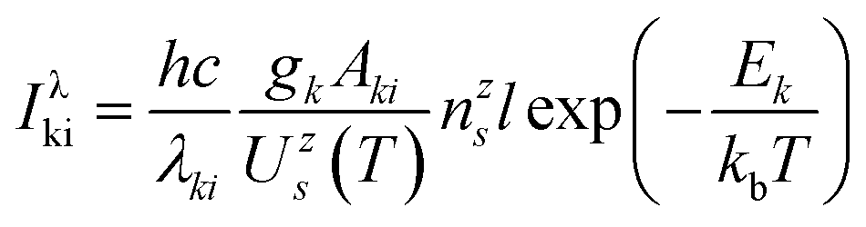 | (1) |
To construct the Boltzmann plot, eqn (1) is rearranged and linearized with respect to Ek using the logarithmic function
 | (2) |
Inserting the units into eqn (2) gives
 | (3) |
The analysis and reduction of units to basic ones in eqn (3) shows that while the second term in the right-hand side is dimensionless, the expressions under the logarithms are dimensioned (kg m s−2) that is unacceptable for a transcendental function like the logarithm. To correct this and rewrite eqn (2) in the dimensionless form, both sides of eqn (1) should be normalized to the unit radiance  to yield
 | (4) |
The numeric values of h0, c0, λ0, A0, n0, and l0 can be taken equal to unity and expressed in the same system of units (e.g., SI) as that in the original expression eqn (1). Rearranging eqn (4) into the form of eqn (2), one obtains the usual Boltzmann plot equation, but with dimensionless arguments under the logarithm
 | (5) |
Obviously, the normalization to the unit radiance does not change the original value of the radiance in eqn (1); it only converts it into the dimensionless form. Furthermore, eqn (5) implies that the abscissa of the plot  versus Ek has the unit of energy and the ordinate is unitless. For convenience and compactness, eqn (5) can be written as eqn (2), but with the understanding that the argument of the logarithmic function is normalized to the chosen system of units.
Most importantly, in practice, the response function must be calibrated in physical units (W m−2) to be able to use the Boltzmann plot equation. However, this limitation can be removed if the Boltzmann plot is built for a narrow spectral range (flat response function), and all spectral lines are normalized to some standard line from this range. In this case, the Boltzmann plot equation becomes dimensionless expressed by
 | (6) |
Here, the reference line is marked with index r and the constants h, c and path length l are truncated.
A commonly used variant of the Boltzmann plot is the Saha–Boltzmann plot, which provides a more accurate temperature determination because it covers a wider range of upper transition energies. This is achieved by combining atomic and ionic species in a single plot by expressing the corresponding number densities through the Saha equation2
 | (7) |
 | (8) |
Note that the expression under the logarithm in the second term on the left-hand side is dimensionless.
3 Error analysis due to inconsistent physical units
To investigate possible errors that can occur when using inconsistent units in the construction of a Boltzmann plot, several possible situations are analyzed. All tested scenarios assume a two-point Boltzmann plot using the lines in Table 1. The integrated line intensity is calculated from eqn (1) using the polynomial approximation3 for partition functions. The temperature is assumed to be 10![[thin space (1/6-em)]](https://www.rsc.org/images/entities/char_2009.gif) 000 K, the number density of atoms is 1 × 10²² m−3, and the path length is 0.001 m. The points on the Boltzmann plot are calculated from eqn (5).
000 K, the number density of atoms is 1 × 10²² m−3, and the path length is 0.001 m. The points on the Boltzmann plot are calculated from eqn (5).
The first scenario assumes that the emission signal is measured in units of counts, i.e., the spectrometer and detector are not calibrated with a standard light source. If the spectral response function is not flat, then the ratio of the measured intensities at 334.94 nm and 390.05 nm will differ from that emitted by the plasma and, therefore, the temperature determined from the slope of the Boltzmann plot will be incorrect. To analyze a possible error for this case, the spectral response function integrated over the line profile and full solid angle is assumed to be 1 W (m2 counts)−1 in the spectral region around 334 nm and 0.8 W (m2 counts)−1 in the region around 390 nm. By dividing the intensities calculated from eqn (1) by these response function values, the intensities measured by the uncalibrated instrument in units of counts are obtained. After substituting these values into eqn (5) and determining the slope of the Boltzmann plot, a temperature of 7444 K is obtained, which makes a 26% relative error with respect to the original temperature of 10000 K.
In the second scenario, it is assumed that the spectrometer is calibrated, and the emission signal is measured in the physical units of W m−2 but the Boltzmann plot equation is calculated using the non-SI system unit of nm for central wavelengths of emission transitions. In this case, the temperature will be determined correctly because the ordinates of all points on the Boltzmann plane will be shifted vertically to equal distances. However, it should be emphasized that the use of inconsistent units in this case is physically incorrect, leading to the appearance of a unit conversion factor under the sign of the logarithm, which, without changing the slope of the function, will shift its intersection point with the y-axis; such the shift may be undesirable in some applications.
Common to all scenarios is that the use of inconsistent units in the Boltzmann plot equation is incorrect from both mathematical and physical points of view and can lead to erroneous temperature values when using the Boltzmann plot method.
4 Conclusion
Since many papers using the Boltzmann method to measure plasma temperature do not check the dimension of the sublogarithmic expression, this technical note emphasizes that such a check is necessary to obtain the correct temperature value. In this context, attention was drawn to the following:(i) Transcendental functions such as the logarithm require a dimensionless quantity as an argument. This can be achieved by normalizing the equation for the integral line intensity by the unit intensity in the chosen system of units that makes the argument of the logarithm dimensionless. This requires calibration of the spectrometer and detector so that the emission signal can be measured in physical units.
(ii) The abscissa on a Boltzmann plot graph has units of energy, and since the logarithmic function gives a dimensionless unit as the value of the function, the ordinate of the Boltzmann plot graph is therefore dimensionless.
It is also shown that the use of inconsistent units of variables and constants in the argument of the logarithmic function can lead to erroneous temperature values when using the Boltzmann plot method. Several scenarios are considered, including the use of uncalibrated measurements or inconsistent units in a sublogarithmic expression. Therefore, it is recommended to carefully analyze the dimension of the quantity under the sign of the logarithm and use agreed units of measurement based on one or another system of physical units (SI, CGS, etc.).
Author contributions
Tobias Völker: conceptualization, methodology, writing – original draft, writing – review & editing, Igor B. Gornushkin: conceptualization, methodology, writing – review & editing. All authors have read and agreed to the published version of the manuscript.Conflicts of interest
The authors declare that they have no known competing financial interests or personal relationships that could have appeared to influence the work reported in this paper.Acknowledgements
The authors are grateful to Dr E. Niederleithinger and Dr J. Riedel for their continued support of this collaborative work. The authors would like to thank the unknown reviewers for taking the time and effort to review the manuscript and provide valuable comments and suggestions.References
- C. F. Matta, L. Massa, A. V. Gubskaya and E. Knoll, J. Chem. Educ., 2010, 88, 67–70 CrossRef.
- W. Lochte-Holtegreven, Plasma Diagn., 1968, 15, 153 Search PubMed.
- A. W. Irwin, Astrophys. J., Suppl. Ser., 1981, 45, 621 CrossRef CAS.
- A. Kramida, Y. Ralchenko, J. Reader and NIST ASD Team, NIST Atomic Spectra Database (version 5.9), National Institute of Standards and Technology, Gaithersburg, 2021 Search PubMed.
| This journal is © The Royal Society of Chemistry 2022 |