 Open Access Article
 This Open Access Article is licensed under a
 Creative Commons Attribution 3.0 Unported Licence
Quench–drive spectroscopy of cuprates
Matteo
Puviani
 * and
Dirk
Manske
* and
Dirk
Manske
Max Planck Institute for Solid State Research, 70569 Stuttgart, Germany. E-mail: m.puviani@fkf.mpg.de
First published on 2nd March 2022
Abstract
Cuprates are d-wave superconductors which exhibit a rich phase diagram: they are characterized by superconducting fluctuations even above the critical temperature, and thermal disorder can reduce or suppress the phase coherence. However, photoexcitation can have the opposite effect: recent experiments have shown an increasing phase coherence in optimally doped BSCCO with mid-infrared driving. Time-resolved terahertz spectroscopies are powerful techniques to excite and probe the non-equilibrium states of superconductors, directly addressing collective modes, such as amplitude (Higgs) oscillations. In this work, we calculate the full time evolution of the current generated by a cuprate with a quench–drive spectroscopy setup. Analyzing the response in Fourier space with respect to both the real time and the quench–drive delay time, we look for the signature of a transient modulation of higher harmonics, as well as the Higgs mode, in order to characterize the ground state phase. In particular, this approach can provide a smoking gun for induced or increased phase coherence when applied to the pseudogap phase. These results can pave the way for future experimental schemes to characterize and study superconductors alongside incoherent phases and phase transitions, including induced and transient superconductivity.
1. Introduction
High-temperature superconductors have attracted much of the attention in the research on superconductivity since their discovery. In recent years, experiments on high-temperature superconductors have revealed the presence of signatures of superconducting fluctuations above the critical temperature Tc. This behaviour has been attributed to incoherent or pre-formed Cooper pairs, leading to third-harmonic generation (THG) and enhancement of the reflectivity change in a pump–probe experimental configuration.1–3Cuprates are the prototypical example of high-temperature superconductors, exhibiting a complex phase diagram as a function of doping and temperature, with a superconducting dome enriched by charge-density wave and pseudogap phases.4 In fact, optimally doped Y-Bi2212 exhibits a superconducting phase below Tc = 97 K, and a pseudogap phase above Tc and up to the temperature T* ≈ 135 K.1,5–8 It has been argued that the pseudogap phase on top of the superconducting dome at optimal doping in unconventional superconductors is driven by the loss of phase coherence between the Cooper pairs, rather than the softening or vanishing of the pairing strength.9–11 Therefore, in the pseudogap phase, the electrons are still paired, but their local phase is different from the global phase of the order parameter, which is lowered as a consequence.
A variety of non-equilibrium experiments on cuprates have indicated the importance and the interaction between collective modes, such as the amplitude (Higgs) mode and Josephson plasmon; different setups have been used to investigate this, from high-harmonic generation to pump–probe spectroscopy, to reflectivity measurements.2,3,12–14 Moreover, it has been recently shown that THz pulses in the mid-infrared region can dynamically enhance the phase coherence of Cooper pairs in optimally doped cuprates, which is lowered by thermal disorder in equilibrium conditions.7
In this paper, we go beyond previous works of pump–probe spectroscopy on cuprates, applying the quench–drive spectroscopy setup15–18 (see Fig. 1) recently extended to study different features of superconductors,19 to superconductors with anisotropic d-wave order parameters. In this configuration, a first few-cycle THz broadband pulse (quenching, red in Fig. 1) impinges on the material, followed after an adjustable delay time, Δt, by a multi-cycle THz narrow-band (asymmetric) driving pulse (driving, green in Fig. 1). Then, the generated current, which is experimentally addressed by measuring the change of the transmitted electric field or the nonlinear optical conductivity,20,21 can be analyzed in transmission in real time after filtering out the linear response directly proportional to the incoming pulses. Quench–drive spectroscopy has been shown to be a versatile and powerful tool to systematically analyze the superconducting response, as well as characterizing the signatures of collective modes, possibly enhancing the overall measured signal.19 This method goes beyond standard pump–probe spectroscopy, where a short-time pulse drives the system out of equilibrium, followed by a subsequent weak and short-time pulse which probes the system (e.g., current, reflectivity).22,23 In a quench–drive setup, in fact, both the short-time pulse and the long-time drive can perturb the system, and the non-fixed relative geometry of the two pulses allows to shift the quench–drive time delay. This provides an extended number of possible configurations, allowing for the quenching pulse to overlap with the driving pulse , or even acting on the driven superconductor after the longer pulse. The analysis of the generated nonlinear current in both time and Fourier space, for example, including not only the real evolution but also the time-dependence of the quenching and driving relative time, allows us to obtain a richer signal than the usual harmonic response of the non-equilibrium material. In fact, the application of this spectroscopic technique to conventional clean s-wave superconductors has demonstrated that it can provide the nonlinear current signal due to the quasiparticles’ and collective modes’ excitations, visible as distinctive features in the two-dimensional time and frequency plots, respectively.19 Alongside the high-harmonic generation, both transient excitation and dynamical modulation of the generated harmonics are visible, and can be theoretically described by solving the real-time Heisenberg’s equation of motion, or interpreted with a diagrammatic approach.
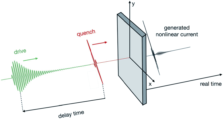 | ||
| Fig. 1 Quench–drive setup. The figure shows the scheme of the quench–drive setup used here: the quenching pulse (red) impinges on the material (grey). Then, after a delay time (Δt, measured from the maximum peak of the quench to the maximum peak of the drive) the driving pulse also interacts with the material; the nonlinear current output is then generated and can be detected in real time. | ||
However, in quench–drive spectroscopy, the real and delay times are not fully independent, since they both refer to the driving pulse, and are not able to catch the decoherence processes. This mainly differs from other three-pulse techniques, like pump–dump–probe, pump–push–probe or pump–repump–probe mechanisms, which have been widely used to study molecular excitations and transient states for decades.24–27 In pump–repump–probe spectroscopy, for example, the first pulse creates a macroscopic polarization which decays due to dephasing, then the second one induces a population of the excited state, while the probe converts it back to a coherent polarized state.28 An extension of our scheme to a real two-dimensional coherent spectroscopy, with two independent times and probing of decoherence processes, will be the object of a future work.
In the present work, we numerically solve the Heisenberg’s equation of motion, derived within the pseudospin formalism,29,30 in order to describe the superconducting state, and we support our interpretations and results with the derivation of the nonlinear susceptibility by means of a diagrammatic approach.31 Moreover, in order to treat the pseudogap phase, characterized by incoherent pairs, we extend the pseudospin model, artificially adding a phase to the Cooper pairs,1 and solving the corresponding equations to obtain the time-evolution of the order parameter and the generated nonlinear current (see Fig. 2(b) and (c)).
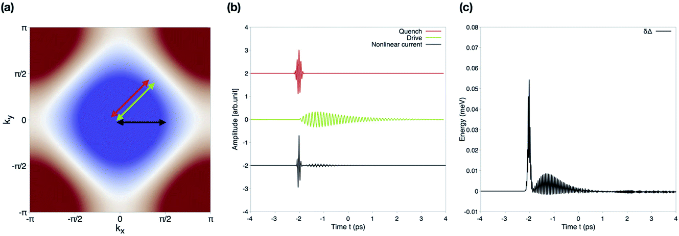 | ||
| Fig. 2 Quench–drive spectroscopy. (a) Band structure in the first Brillouin zone used to reproduce the optimally doped Bi2212; the red and green arrows represent the direction of linear polarization of the quenching and driving pulses, respectively. The black arrow indicates the direction of the measured current, i.e. along the x axis. (b) The figure shows the external vector potential of the quenching (red) and the driving (green) pulses for an example case with fixed quench–drive delay time, as well as the nonlinear current response (black). (c) Time-dependent superconducting order parameter variation, δΔ(t) = Δ(t) − Δ(0), due to the quenching and driving pulses in (b). | ||
The paper is organized as follows: in Section 2, we describe the theoretical models that we used. Starting from the pseudospin approach to solve the equations of motion in order to calculate the time-dependent superconducting gap and the generated nonlinear current, we extend it in order to be able to describe incoherent pairs. In addition, we perform the same calculations for the superconducting state using a diagrammatic approach, deriving the nonlinear susceptibility responsible for the measured response. In Section 3, we show the results of the numerical experiments for the quench–drive setup on a cuprate: we analyze the two dimensional plots in the time and frequency domains, detecting the presence of higher harmonics and signatures of quasiparticles’ and the Higgs mode. Then, we repeat the calculation in the presence of incoherent pairs: we show that even a moderate incoherence, which only slightly reduces the superconducting gap, can suppress the high-harmonic generation in the nonlinear current, as well as the quasiparticles’ and amplitude mode’s response. Finally, we provide a summary and an outlook on future applications and perspectives of quench–drive spectroscopy in Section 4.
2. Theoretical background
In this section, we formulate the theoretical approach used to investigate the current generated by a clean (high-temperature) superconductor subject to an external field. We first develop the pseudospin model for a general superconductor, then we extend it in order to be able to describe incoherent pairs. Finally, we show a diagrammatic approach, where we derive the nonlinear susceptibility used to obtain the nonlinear current, disentangling the quasiparticles’ and Higgs’ contributions.2.1 Pseudospin model approach
In order to describe the superconducting phase of a material, we adopt the BCS model expressed by the mean field Hamiltonian: | (1) |
 | (2) |
 . Therefore, it follows from eqn (2) that the gap function itself can be factorized as Δk = Δ0fk.
We write the BCS Hamiltonian using the pseudospin formalism, as in ref. 30 and 32, namely
 | (3) |
 | (4) |
![[capital Psi, Greek, circumflex]](https://www.rsc.org/images/entities/i_char_e0b0.gif) †k = (ĉ†k,↑ĉ−k,↓) and the Pauli matrices τ = (τ1, τ2, τ3). The pseudo-magnetic field is defined by the vector
†k = (ĉ†k,↑ĉ−k,↓) and the Pauli matrices τ = (τ1, τ2, τ3). The pseudo-magnetic field is defined by the vector| bk = (−Δ′fk, −Δ′′fk, εk), | (5) |
In the presence of an external gauge field represented by the vector potential A(t) coupling to the electrons, the pseudospin changes in time according to
| σk(t) = σk(0) + δσk(t), | (6) |
| bk(t) = (−Δ′(t)fk, −Δ′′(t)fk, εk−eA(t) + εk+eA(t)). | (7) |
The Heisenberg equation of motion for the pseudospin can be written in the Bloch form, ∂tσk = 2bk × σk, providing the set of differential equations
 | (8) |
Moreover, in order to describe a quench–drive experiment, we choose the appropriate total vector potential A(t) = Aq(t) + Ad(t) = Āq(t − tq) + Ād(t − td), where Aq(t) is the quenching pulse centered at time t = tq and Ad(t) is the driving field centered at t = td. The expression we used for the modulus of the quenching pulse is a Gaussian-modulated wave,
 | (9) |
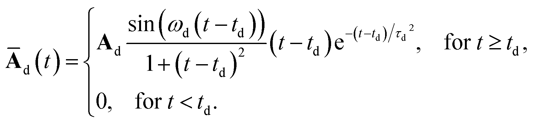 | (10) |
By introducing the quench–drive time-delay Δt = td − tq and choosing td = 0, we can rewrite A(t) = Āq(t + Δt) + Ād(![[t with combining macron]](https://www.rsc.org/images/entities/i_char_0074_0304.gif) ). Therefore, the expressions in eqn (6)–(8) depend on both t and Δt.
). Therefore, the expressions in eqn (6)–(8) depend on both t and Δt.
The solution of eqn (8) provides the full time-dependent pseudospin, from which the time-dependent order parameter Δ(t) can be calculated, namely
 | (11) |
 | (12) |
 | (13) |
However, since the fundamental harmonic is dominant in this regime, while the superconducting features are visible in the nonlinear response, we are interested in the lowest order nonlinear current contribution. The first non-vanishing nonlinear term generated by the driving pulse is the third order component, which reads
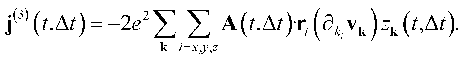 | (14) |
By identifying the factor depending on the derivative of the velocity and the direction of the external field with Cx(k), we can write the x component of the third harmonic generated current as
 | (15) |
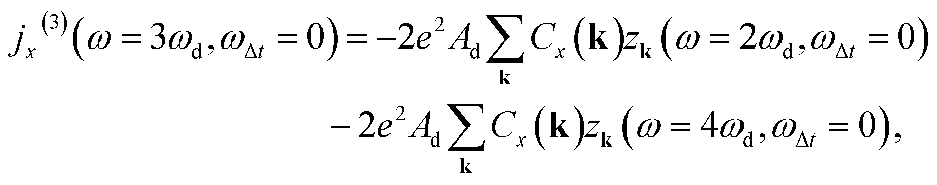
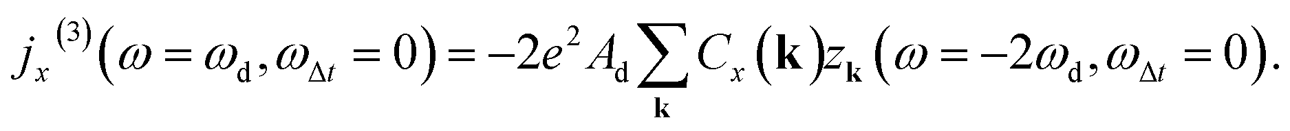 | (16) |
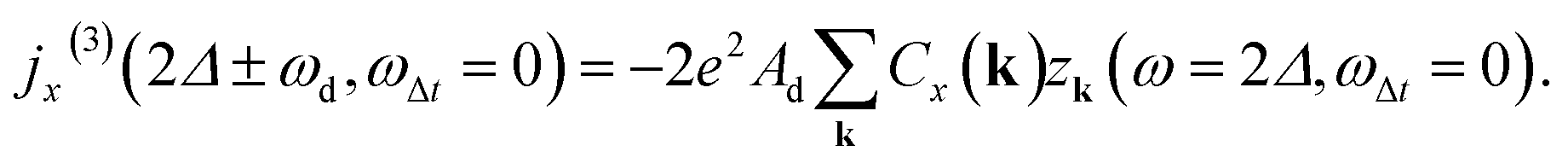
Moreover, since the third component of the pseudospin has a (non-resonant) peak in the frequency domain at ω = 2Δ, it is possible to obtain other local maxima for the generated nonlinear current at ω = 2Δ ± ωd:
 | (17) |
In addition to these contributions, other terms which involve the quenching pulse are present, such as – among others – the nonlinear current term,
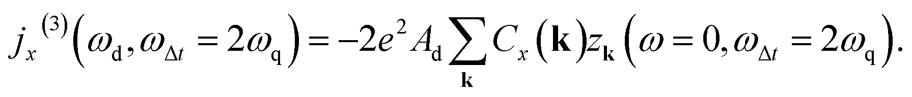 | (18) |
This expression involves a sum-frequency process of two photons of the quenching pulse, each with frequency ωq, embedded in the third component of the pseudospin, zk, thus, the dependence zk(ωΔt = 2ωq), and it also implicitly depends quadratically on the amplitude of the quenching pulse, Aq2.
2.2 Extended pseudospin model for incoherent pairs
We now want to describe a state with a superconducting instability and characterized by the presence of pre-formed incoherent pairs, which can be identified as the origin of the pseudogap phase; in this regard, as in ref. 1, we use a new artificial equilibrium superconducting state obtained by adding a random momentum-dependent phase ϕk to the original Cooper pairs’ state. Therefore, the strength of the pairing potential remains unchanged, as well as the number of total Cooper pairs, while the superconducting order parameter decreases due to the reduced coherence. According to the maximum angle ϕmax, which defines the range of the random phase ϕk, with ϕk ∈ [−ϕmax, +ϕmax], we are able to describe different conditions of the material, from the pure superconducting phase for ϕmax = 0 to the complete loss of coherence for ϕmax = π.We define the gap of the pure superconducting state Δ(0)k = Δ(0)0fk, obtained from the pure BCS gap equation, and the superconducting order parameter in the presence of incoherent pairs of the pseudogap phase as ![[capital Delta, Greek, tilde]](https://www.rsc.org/images/entities/i_char_e10b.gif) k(ϕ) = (ϕ)fk, such that
k(ϕ) = (ϕ)fk, such that
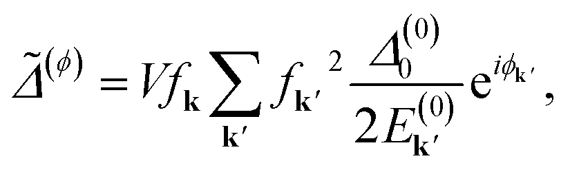 | (19) |
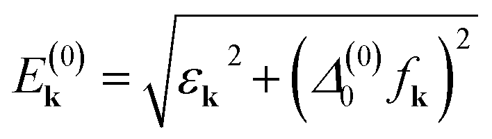 . The superconducting gap in the new equilibrium state can be written using the pseudospin formalism
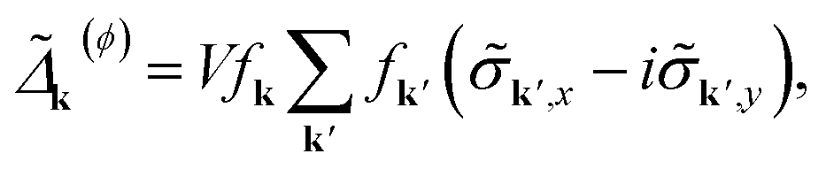 | (20) |
 | (21) |
Analogously to the derivation in Section 2.1 for the original superconducting phase, we can obtain the Heisenberg’s equation of motion
∂t![[small sigma, Greek, tilde]](https://www.rsc.org/images/entities/i_char_e10d.gif) k = k = ![[b with combining tilde]](https://www.rsc.org/images/entities/b_char_0062_0303.gif) × k, × k, | (22) |
| = (−′fk, −′′fk, εk). | (23) |
The solution of eqn (22) provides the time-dependent value of the pseudospin k, from which the evolution of the new order parameter (ϕ) can be obtained. However, we notice that the complex order parameter can be written as
| (ϕ) = |(ϕ)|eiθ, | (24) |
2.3 Quasi-equilibrium nonlinear susceptibility
In this section, we tackle the problem of a quenched–driven clean superconductor by means of a diagrammatic approach to calculate the nonlinear susceptibility; this is provided only as a tool to interpret the numerical results obtained via the pseudospin model.Starting from the BCS Hamiltonian in eqn (1), we add the interaction of the external field that we treat perturbatively, which can be expressed as a sum of the Feynman diagrams around a quasi-equilibrium condition. In particular, the current generated by the perturbed superconductor in the quasi-equilibrium condition satisfies a proportionality relation with the generalized density–density susceptibility, namely j(ω) ∼ χγγ(ω′)A3(ω − ω′), with χγγ(ω) = 〈![[small rho, Greek, tilde]](https://www.rsc.org/images/entities/i_char_e0e4.gif) 〉 and
〉 and 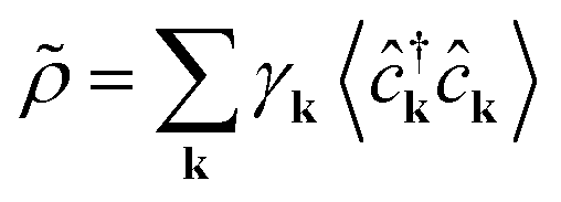 .
.
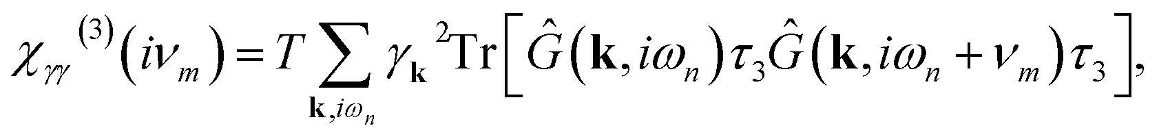
Since we are considering a clean superconductor, the lowest non-vanishing order of the nonlinear response is provided by the third-order nonlinear susceptibility χγγ(3)(ω),31 where γk is the diamagnetic light–matter (vertex) interaction strength, which can be written in the effective mass approximation as 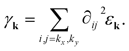 33,34
33,34
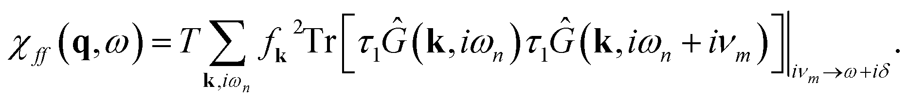
The pure quasiparticles’ diamagnetic response is given by the bare density–density susceptibility, which in Nambu notation within the Matsubara formalism reads
 | (25) |
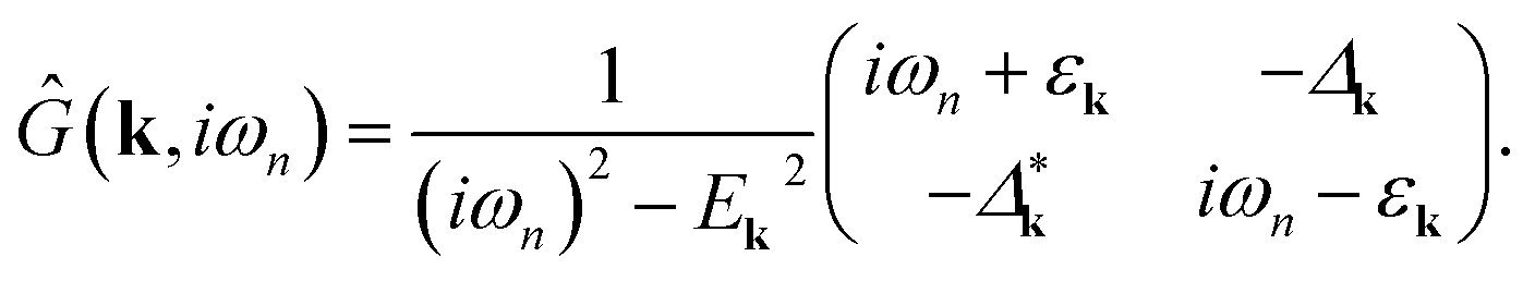 | (26) |
This function can be expressed in its spectral form as
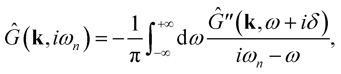 | (27) |
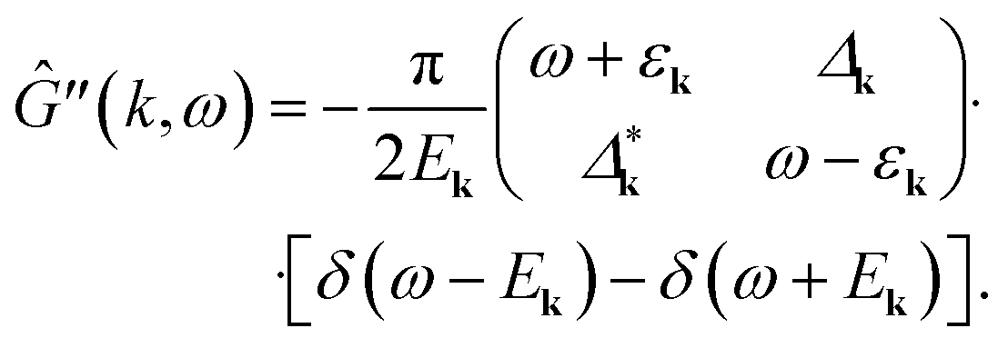 | (28) |
Therefore, the expression in eqn (25) can be solved, obtaining
 | (29) |
This is the pure quasiparticles’ contribution, obtained by neglecting the oscillations of the order parameter for small perturbations. The Higgs propagator is obtained by the random phase approximation (RPA) summation of the pairing interaction in the amplitude channel:
| DHiggs(q, ω) = −V/2 − V/2χff(q, ω)DHiggs(q, ω), | (30) |
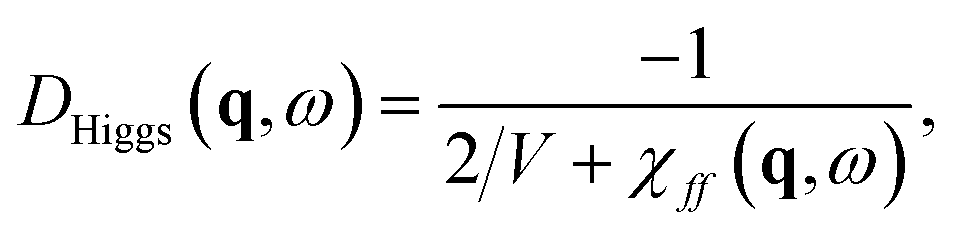 | (31) |
 | (32) |
We can include in the pure quasiparticles’ Raman response in eqn (25) the Higgs contribution given by the propagator in eqn (31), obtaining the full Raman response
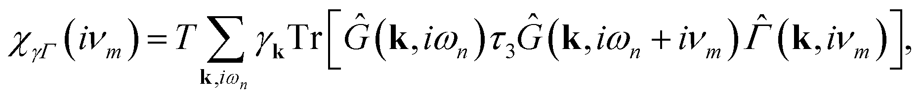 | (33) |
![[capital Gamma, Greek, circumflex]](https://www.rsc.org/images/entities/i_char_e132.gif) (k, iνm) is the vertex matrix, which contains the corrections due to the Higgs mode. In the RPA, we can identify it as
(k, iνm) is the vertex matrix, which contains the corrections due to the Higgs mode. In the RPA, we can identify it as | (34) |
Additional corrections can be included in this vertex with different forms.
The linearized equations of motion obtained by removing higher-order terms in eqn (8) provide the same result of the nonlinear susceptibility calculated from the diagrammatic contributions of the density–density response including the RPA summation of the amplitude mode, responsible for the value of δΔ(ω). The real part of the oscillation of the order parameter, namely the amplitude (Higgs) mode, reads in frequency space
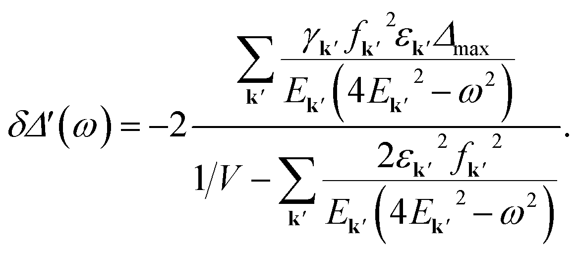 | (35) |
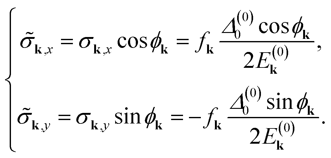
The vertex in eqn (34) after analytic continuation of the complex Matsubara frequency can be written, including explicitly the amplitude mode in eqn (35), as (k, ω) = γkτ3 + δΔ′(ω)fkτ1.
The expression of the vertex factor γk depends on the symmetry of the response which is measured; however, if we consider the experimental configurations with linearly polarized light along high-symmetry crystallographic directions, we can replace the factor γk with the tensor γij(k) = ∂ij2εk, and define the corresponding susceptibility from eqn (25) as follows:
 | (36) |
For example, for quenching and driving pulses with nonzero components along both the x and y directions, the third-order nonlinear response current generated along the x axis will be given by
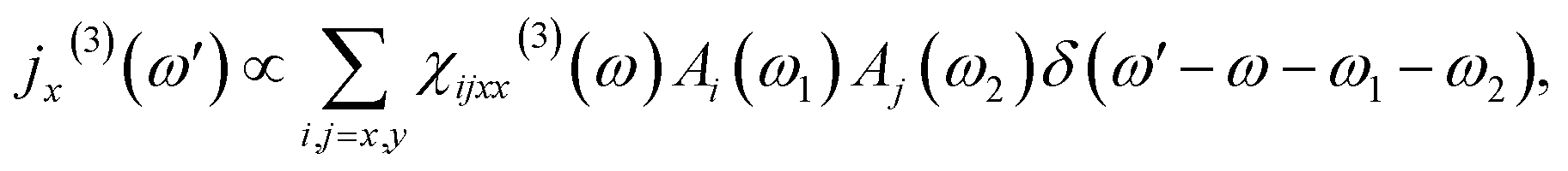 | (37) |
We notice that, in contrast to the solution of the Heisenberg’s equations of motion which are valid on a general basis, the diagrammatic approach is valid for small perturbations of the superconducting order parameter Δ. Therefore, when the intensity of the external pulses is such that the gap is significantly enhanced or suppressed, so that a new (transient) equilibrium value of the gap Δ′ is reached, the quasi-equilibrium susceptibility calculation fails to catch all the features of the corresponding nonlinear response, requiring a full non-equilibrium calculation.
Moreover, this approach cannot be easily applied when pre-formed pairs or superconducting islands are present in the material, such as in the pseudogap phase of a cuprate, giving rise to long-range incoherence of the Cooper pairs.
3. Numerical results
We now present the results obtained from the numerical implementation of the time-dependent Bloch equations and expressions for the current derived from the pseudospin model in Sections 2.1 and 2.2. For the calculations, we used the electronic band dispersion εk = −2t(cos![[thin space (1/6-em)]](https://www.rsc.org/images/entities/char_2009.gif) kx + cosky + μ/2), where the wave vector’s components are expressed in units of the lattice constant a. We used the values of t = 125 meV for the nearest-neighbour hopping energy and chemical potential μ = −0.2, in units of t, in order to obtain an electron occupation n = 0.9, as in ref. 1; the corresponding band structure is shown in Fig. 2(a). For the d-wave order parameter with symmetry Δk = Δmax(coskk − cosky)/2, we adopted the value Δmax = 31 meV; the calculations were performed with a summation over the full Brillouin zone with a homogeneous square sampling and a total number of k points Nk = 106. For the time-dependent evolution, we used a time-step of δt = 3 × 10⁻⁴ ps, and for the quench–drive delay δΔt = 2.5 × 10⁻² ps.
kx + cosky + μ/2), where the wave vector’s components are expressed in units of the lattice constant a. We used the values of t = 125 meV for the nearest-neighbour hopping energy and chemical potential μ = −0.2, in units of t, in order to obtain an electron occupation n = 0.9, as in ref. 1; the corresponding band structure is shown in Fig. 2(a). For the d-wave order parameter with symmetry Δk = Δmax(coskk − cosky)/2, we adopted the value Δmax = 31 meV; the calculations were performed with a summation over the full Brillouin zone with a homogeneous square sampling and a total number of k points Nk = 106. For the time-dependent evolution, we used a time-step of δt = 3 × 10⁻⁴ ps, and for the quench–drive delay δΔt = 2.5 × 10⁻² ps.
For the pulses, we used a Gaussian-shaped few-cycle qeuenching and an asymmetric long-duration driving pulse, as expressed in eqn (9) and (10) and shown in Fig. 2(b), linearly polarized along the (1, 1) direction (Fig. 2(a)), with parameters τq2 = 0.01 ps2 and τd2 = 5 ps2, respectively. The maximum intensity used for each pulse is provided for the corresponding vector potential in units of ℏ/(ea), where e is the electron charge and a the lattice constant; the conversion to the value of the electric field for each frequency is provided in Table 1. Table 2 reports the conversion of each frequency (in THz) of the pulses used for the calculations to the energy scale (in meV).
| Frequency (THz) | A max | E max (kV cm−1) |
|---|---|---|
| 4.57 | 0.4 | 22.3 |
| 5.09 | 1.6 | 99.3 |
| 7.16 | 0.2 | 17.5 |
| 7.16 | 0.4 | 35.0 |
| 7.80 | 0.8 | 76.1 |
| 8.28 | 0.4 | 40.4 |
| 11.14 | 0.8 | 109 |
| 12.73 | 0.8 | 124 |
| Frequency (THz) | Energy (meV) |
|---|---|
| 4.57 | 18.90 |
| 5.09 | 21.05 |
| 7.16 | 29.61 |
| 7.80 | 32.26 |
| 8.28 | 34.24 |
| 11.14 | 46.07 |
| 12.73 | 52.65 |
3.1 Quench–drive response of the superconducting state
We first focus on the response of a cuprate in its superconducting phase, at optimal doping; in particular, we first analyze the features of the current response as a function of both the real-time evolution and the quench–drive delay time. Then, we investigate the effect of both the quenching and driving pulses on the superconducting order parameter and its amplitude oscillations.In Fig. 3(a), we show the nonlinear current jNL(t, Δt) generated by the superconductor as a function of the real evolution time t and for different quench–drive delay times, labeled as Δt. The diagonal line represents the current induced by the quenching pulse, while the vertical signal is due to the asymmetric driving field which sets in at time t = −2 ps. The triangular area for 0 ≥ t ≥ Δt, for Δt ∈ [−2, 0] ps is characterized by a response due to the overlap (wave mixing) of both the quenching and driving pulses.
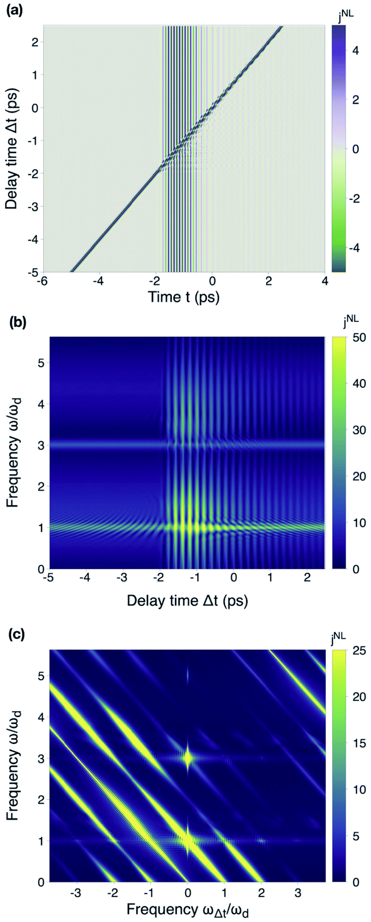 | ||
| Fig. 3 Two-dimensional plots of the generated nonlinear current. (a) Nonlinear current response, j,NL as a function of real time, t, and quench–drive delay time, Δt. The quenching frequency is ωq = 7.80 THz, the driving frequency ωd = 5.09 THz, while the maximum gap value Δmax = 31 meV. The maximum intensities of the pulses used were Aq = 0.8 and Ad = 1.6, respectively. The diagonal line represents the current due to the quenching pulse, while the vertical lines correspond to the oscillations induced by the asymmetric driving field, which sets in at t = −2 ps. (b) The figure corresponds to the same in (a), where the horizontal axis of the real time t has been Fourier transformed to ω, whose values are referred to as the drive frequency ωd. (c) 2D Fourier transform of the signal in (a), representing the nonlinear current as a function of ω and ωΔt. | ||
A Fourier analysis of this plot can provide information about the harmonics present in the current itself. In Fig. 3(b), we present the same results as a function of the frequency ω, obtained by Fourier transforming the time evolution, t, and the delay time, Δt. We can clearly distinguish the fundamental and the third generated harmonic, which are modulated by the delay time as the quenching is swiped with respect to the driving field. This is in accordance with previous theoretical findings on conventional s-wave superconductors.19 However, we also observe that faded modulated responses appear for Δt > −2 ps, both at frequencies slightly higher than ωd and 3ωd, respectively; they also show a modulation in the delay time, as with the other two aforementioned harmonics. Since their appearance and intensity modulation match the time at which the driving field sets in, these features can be attributed to the wave mixing pattern due to the overlap in time of the quenching and the driving fields.
In Fig. 3(c), the full two-dimensional Fourier transform of the nonlinear current is shown, with the frequency scales referring to the driving frequency ωd. The bright spots along the vertical axis at ωΔt = 0 correspond to the static harmonics generated by the driving field only, while the diagonal stripes are given by wave mixing of the quenching and the driving pulses.
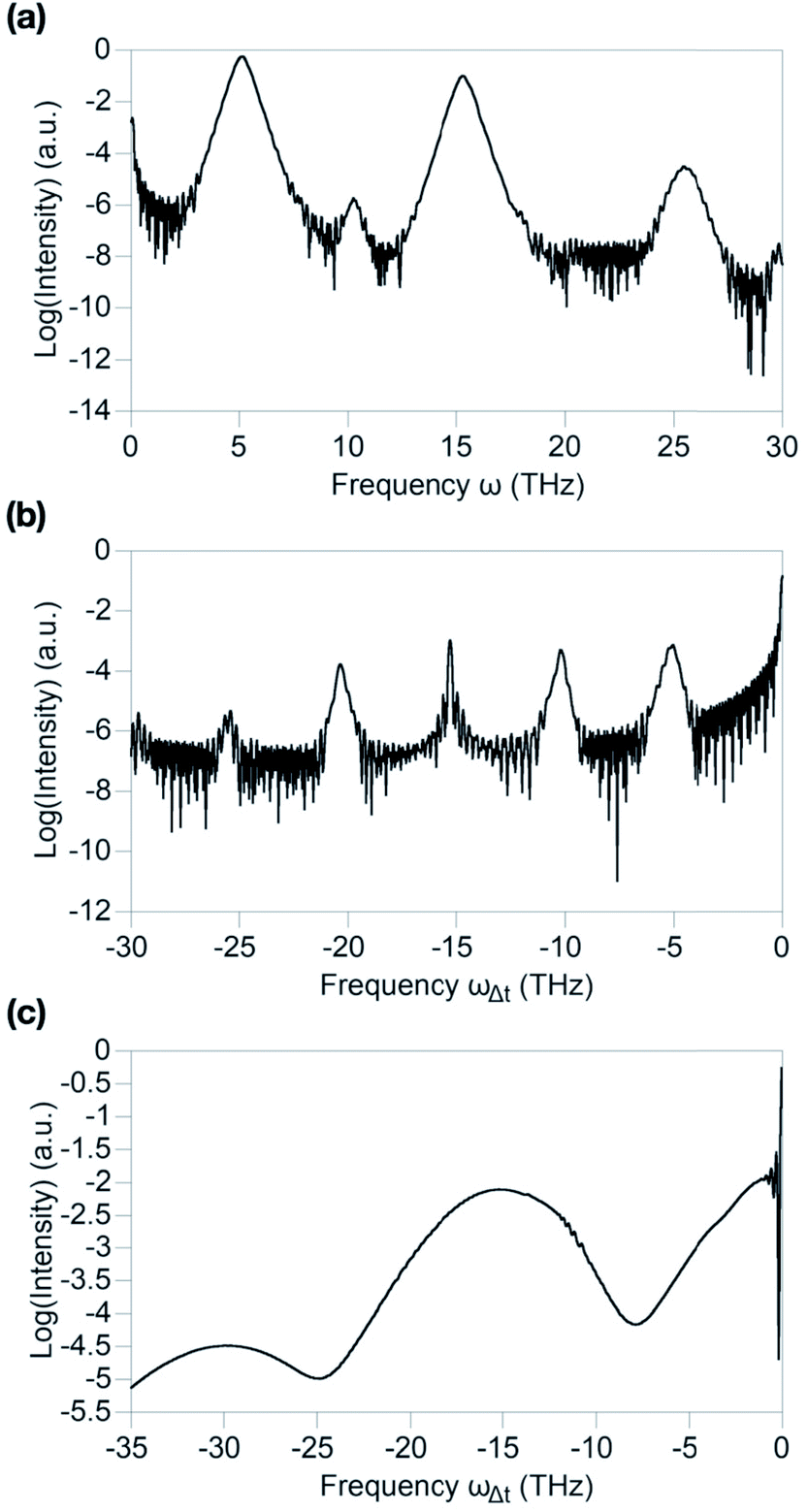 | ||
| Fig. 4 One dimensional plots of the nonlinear current. Plots of the nonlinear current jNL extracted from Fig. 3(c) along some relevant directions. (a) Current spectrum for ωΔt=0 as a function of ω, corresponding to a vertical cut in the two-dimensional Fourier spectrum. (b) Spectrum of the modulation of the third harmonic (TH), corresponding to a cut at ω = 3ωd parallel to the x axis. (c) Current intensity for ω = −ωΔt + ωd, corresponding to the diagonal feature in Fig. 6(a), starting from the fundamental harmonic at ω = ωq, ωΔt = 0. | ||
In Fig. 4(b), we present the spectrum of the generated third harmonic with respect to the absorption frequency, ωΔt; this corresponds to tracking the values at ω = 3ωd, parallel to the horizontal axis, or, equivalently, to analyze the modulation spectrum of the third harmonic in Fig. 3(b). In fact, the third harmonic signal is modulated by the quench–drive delay time, with intensity peaks at frequencies of multiples of ωd. However, the peak at ωΔt ≈ 15 THz is particularly sharp with respect to the others because of the resonance condition with the quasiparticles’ and Higgs energies 2Δmax being Δmax = 31 meV ≈ 7.5 THz. Therefore, the dynamical modulation of the third harmonic is here enhanced by the transient excitation of quasiparticles and the Higgs mode, the latter of which is responsible for the amplitude oscillation of the order parameter, which will be discussed in the next section. Indeed, the enhancement of the broadband quenching fundamental signal by these two contributions can also be detected in Fig. 4(c), where the track of ω = −ωΔt + ωd from Fig. 5(c) is shown.
In Fig. 5 we compare the gap variation, δΔ, for different parameters of the external fields, plotting them as a function of the time evolution, t, and the delay time of the quenching and driving pulses, Δt.
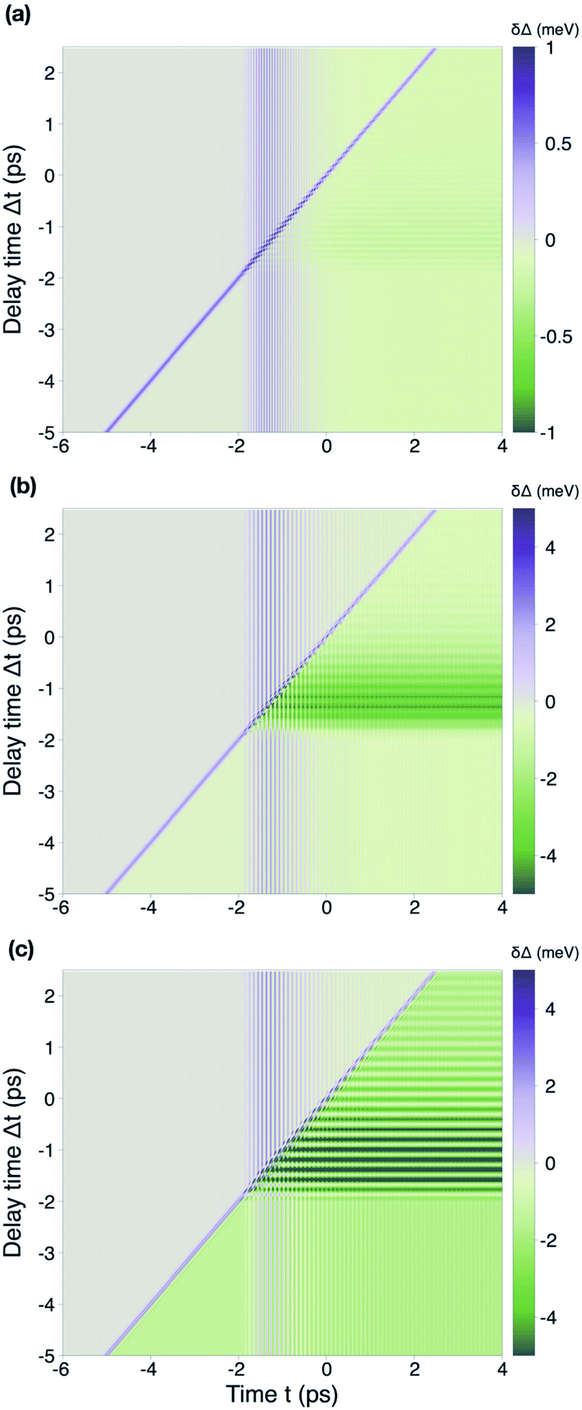 | ||
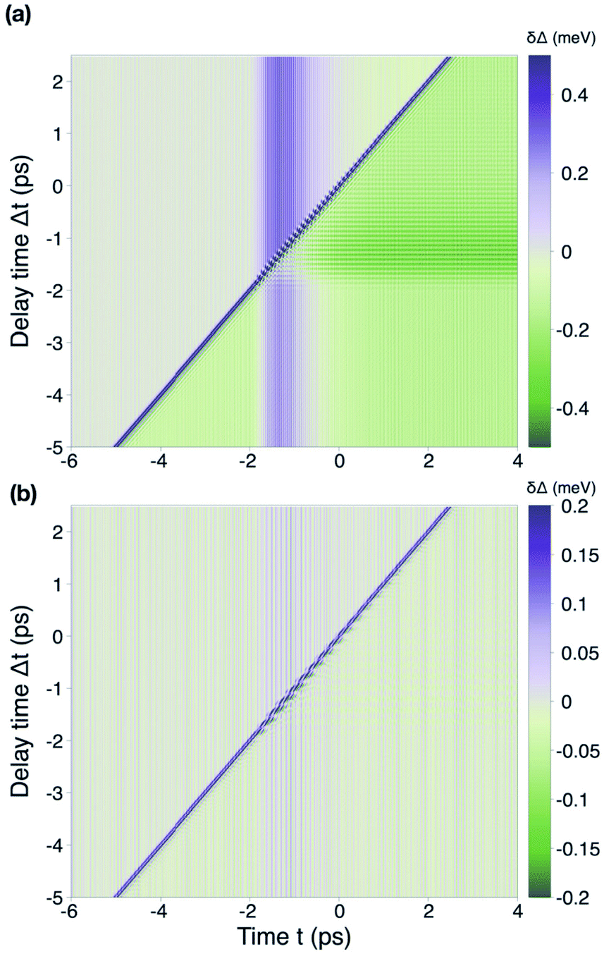
| Fig. 5 Two-dimensional plots of the amplitude mode. The plots represent the amplitude mode, i.e. the variation of the order parameter δΔ(t, Δt) = Δ(t, Δt) − Δmax, as a function of real time, t, and quench–drive delay time, Δt, for different quenching and driving pulses. (a) Quenching frequency ωq = 8.28 THz, intensity Aq = 0.4, driving with ωd = 12.73 THz and Ad = 0.8. (b) Pulse frequencies ωq = 5.09 and ωd = 12.73, intensities Aq = 0.8 and Ad = 1.6. (c) The same parameters as in (b) were used, except for the quenching frequency ωq = 7.80 THz. | ||
In Fig. 5(a), we use a quenching pulse with frequency ωq = 8.28 THz and intensity Aq = 0.4 and a driving pulse with ωd = 12.73 THz and Ad = 0.8. The oscillations of the order parameter have an amplitude δΔmax < 1 meV; they are overall positive for the duration of the quenching pulse and the driving pulse, but they become negative at longer times until a new equilibrium value of the gap (smaller than the initial one) is reached. In Fig. 5(b), the frequencies of the pulses are set as ωq = 5.09 and ωd = 12.73, while their intensities are Aq = 0.8 and Ad = 1.6, respectively. Due to the higher fluence of both pulses, the oscillations of the gap are higher (up to 4–5 meV) and the effect of the pump becomes stronger; even during the time overlap of the quenching and driving pulses, in fact, the gap is suppressed and characterized by an intensity modulation in the delay time, Δt.
As shown in Fig. 5(c), we reduced the quenching frequency to ωq = 7.80 THz, obtaining the same parameters of the calculations of the previous section on the nonlinear current. The suppression of the gap by the quenching pulse is enhanced here due to the approaching of the resonance condition ωq ≈ Δmax, and the intensity modulation in Δt for t > 2 ps, namely when the quenching and the driving pulses overlap, is increased.
Therefore, we can conclude that higher fluences are associated, for higher frequencies, with a suppression of the gap and an enhancement of its oscillations at the same time, which leads to a more intense amplitude mode and a sizeable response in the nonlinear current. On the contrary, for lower frequencies, the gap is transiently enhanced during both the quenching and the driving, in accordance with previous results.1
3.2 Quench–drive response of incoherent pairs
Similarly to the study of the pure superconducting phase of cuprates of the previous section, we now focus on the response of the same cuprate structure in the presence of reduced phase coherent giving rise to pre-formed incoherent Cooper pairs, as described in Section 2.2. In particular, for our calculations, we adopted a random phase within the range [−π/2, π/2], which decreases the initial gap value of Δmax = 31 meV to(ϕ) = 27.92 meV. We also used the same duration and shape parameters for both the quenching and the (asymmetric) driving pulses.
In Fig. 6(a), we show the result for Aq = 0.4, ωq = 7.16 THz, Ad = 0.8 and ωd = 11.14 THz. While a third harmonic generated by the driving field is still present, its intensity is strongly suppressed (notice the log scale used). This is confirmed also by the one dimensional track in Fig. 7(a), which shows a 6 orders of magnitude difference between the first and third generated harmonics.
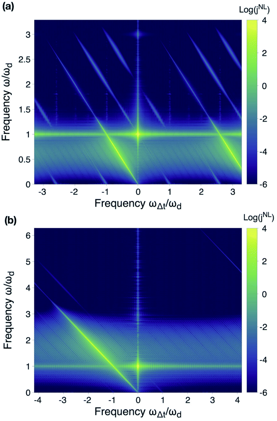 | ||
| Fig. 6 Two-dimensional plots in Fourier space of the generated nonlinear current. (a) Nonlinear current (log scale) generated by the superconductor with quenching intensity Aq = 0.4 and frequency ωq = 7.16 THz, driving intensity Ad = 0.8 and frequency ωd = 11.14 THz. (b) Nonlinear current (log scale) generated by the superconductor with quenching intensity Aq = 0.2 and frequency ωq = 7.16 THz, driving intensity Ad = 0.4 and frequency ωd = 4.57 THz. | ||
 | ||
| Fig. 7 One dimensional plots of the nonlinear current. These plots represent the nonlinear current jNL in log scale extracted from Fig. 6(a) along some relevant directions. (a) Current spectrum for ωΔt=0 as a function of ω, corresponding to a vertical cut in the two-dimensional Fourier spectrum. (b) Spectrum of the modulation of the third harmonic, corresponding to a cut at ω = 3ωd parallel to the x axis. (c) Current intensity for ω = −ωΔt + ωd, corresponding to the diagonal feature in Fig. 6(a) starting from the fundamental harmonic at ω = ωq, ωΔt = 0. | ||
In Fig. 7(b), the spectrum of the TH modulation is shown. While the 2ωd and 4ωd are still present, the peak at 2Δ is suppressed, in contrast to the result of the pure superconducting state (Fig. 4(b)). The same conclusion can be reached from Fig. 7(c), which shows the diagonal track of Fig. 6(a), corresponding to ω = −ωΔt + ωd, where the broadband signal of the quench pulse is visible, which is not enhanced here by the quasiparticles’ and Higgs resonance, in contrast to the pure superconducting case.
If we further decrease the intensity of the pulses, we obtain a complete suppression of the third harmonic with respect to the fundamental, which is shown in Fig. 6(b), where we used Aq = 0.2, ωq = 7.16 THz, Ad = 0.4 and ωd = 4.57 THz. In this case, even approaching the resonance condition ωd ≈ (ϕ), the third harmonic is not present, as well as the dynamical modulation of the harmonics.
In Fig. 8, we present the plots of the time-dependent change of the superconducting order parameter δΔ(t, Δt), corresponding to the same setup conditions of the results in Fig. 6. In particular, we observe that stronger quenching and driving pulses enhance the gap for the duration of the perturbation itself, except when the quenching overlaps in time with the driving field, i.e. t ∈ [−2, 0] ps (see Fig. 8(a)). On the contrary, weak pulses do not significantly enhance the superconducting gap, nor activate amplitude oscillations (Fig. 8(b)). As deduced from the nonlinear current response described in the previous section, the amplitude mode is suppressed by the presence of incoherence in the Cooper pairs; physically, this can be understood by the fact that instead of one coherent amplitude mode with a definite phase, we have a dispersion of modes with different phases and signs, which tend to cancel each other out. Therefore, unless strong pulses increase the superconducting gap and, hence, the phase coherence, the Higgs and quasiparticles’ modes are suppressed.
 | ||
| Fig. 8 Comparison of the time-dependent order parameter. Plot of the time-dependent gap change δΔ(t, Δt), referred to as the equilibrium value. The results shown in panels (a and b) are obtained with the same parameters of the corresponding plots in Fig. 6, respectively. | ||
4. Conclusions
In this work, we have studied the quench–drive spectroscopy response of cuprate superconductors, which are interesting for their anisotropic d-wave superconducting order parameter and their rich phase diagram. In this work, we have explored two different situations: the pure superconducting state and the phase with incoherent pre-formed Cooper pairs, which can reproduce the results of the pseudogap phase, or even originate from other conditions. With this method, we have moved a step forward with respect to previous experiments and calculations, where only a pump (short quenching or longer driving) of cuprates was considered. In fact, in the common pump–probe configuration, only the real time evolution of the system driven out of equilibrium by the pump was tracked by the probe and analyzed. On the contrary, we have shown that in the quench–drive setup, both the short-time and the long-time pulses can act as out-of-equilibrium drivers on the material, affecting both the order parameter and the nonlinear current response. Moreover, this setup has an additional temporal degree of freedom with respect to the pump–probe setup, namely the quench–drive delay time is continuously swiped in order to gain insight into the dependence of the response on the absorption frequency ωΔt. This has allowed us to investigate the high-harmonic generation, the modulation of such harmonics in the quench–drive delay time and the role of the amplitude mode in the features of the nonlinear current. In particular, we have detected a fifth harmonic (visible at ω = 5ωd ≈ 25 THz) generated by the superconductor in some conditions, as well as a peak at the energy 2Δ, which can be attributed to quasiparticles and the amplitude (Higgs) mode, as shown by the analysis of the fluence and frequency dependence of the change of the order parameter.Furthermore, we have applied quench–drive spectroscopy to a cuprate with incoherent pre-formed pairs, artificially adding a random noise phase to the Cooper pairs in momentum space. The results have shown that, even for moderate incoherence, the decrease of the superconducting gap is accompanied by the partial or total suppression of the third harmonic response, as well as the amplitude mode contribution to the nonlinear current. These results can be experimentally addressed and tested by the measurement of the transmitted electric field or the nonlinear optical conductivity.
A more detailed and systematic analysis of the response of incoherent pairs and the amplitude mode of their superconducting gap will be the subject of a future work. We further speculate that an extended configuration, such as a pump–pump–probe scheme, could be used to add an independent time degree of freedom on the real time evolution and the pump–probe delay time, as already used to study molecular excitations and semiconductors.28,36
Conflicts of interest
There are no conflicts of interest to declare.Acknowledgements
Fruitful discussions with P. M. Bonetti, R. Haenel, S. Kaiser, M.-J. Kim, M. Monaco and D. Vilardi are thankfully acknowledged. Open Access funding provided by the Max Planck Society.Notes and references
- F. Giusti, A. Marciniak, F. Randi, G. Sparapassi, F. Boschini, H. Eisaki, M. Greven, A. Damascelli, A. Avella and D. Fausti, Phys. Rev. Lett., 2019, 122, 067002 CrossRef CAS PubMed.
- H. Chu, M.-J. Kim, K. Katsumi, S. Kovalev, R. D. Dawson, L. Schwarz, N. Yoshikawa, G. Kim, D. Putzky and Z. Z. Li, et al. , Nat. Commun., 2020, 11, 1–6 CrossRef PubMed.
- H. Chu, S. Kovalev, Z. X. Wang, L. Schwarz, T. Dong, L. Feng, R. Haenel, M.-J. Kim, P. Shabestari, H. L. Phuong, K. Honasoge, R. D. Dawson, D. Putzky, G. Kim, M. Puviani, M. Chen, N. Awari, A. N. Ponomaryov, I. Ilyakov, M. Bluschke, F. Boschini, M. Zonno, S. Zhdanovich, M. Na, G. Christiani, G. Logvenov, D. J. Jones, A. Damascelli, M. Minola, B. Keimer, D. Manske, N. Wang, J.-C. Deinert and S. Kaiser, Fano Interference of the Higgs Mode in Cuprate High-Tc Superconductors, 2021 Search PubMed.
- B. Keimer, S. A. Kivelson, M. R. Norman, S. Uchida and J. Zaanen, Nature, 2015, 518, 179–186 CrossRef CAS PubMed.
- W. Zhang, C. L. Smallwood, C. Jozwiak, T. L. Miller, Y. Yoshida, H. Eisaki, D.-H. Lee and A. Lanzara, Phys. Rev. B: Condens. Matter Mater. Phys., 2013, 88, 245132 CrossRef.
- E. Baldini, A. Mann, B. P. P. Mallett, C. Arrell, F. van Mourik, T. Wolf, D. Mihailovic, J. L. Tallon, C. Bernhard, J. Lorenzana and F. Carbone, Phys. Rev. B, 2017, 95, 024501 CrossRef.
- F. Giusti, A. Montanaro, A. Marciniak, F. Randi, F. Boschini, F. Glerean, G. Jarc, H. Eisaki, M. Greven, A. Damascelli, A. Avella and D. Fausti, Phys. Rev. B, 2021, 104, 125121 CrossRef CAS.
- A. K. Abdullah Kaplan, Corpus J. Case Rep., 2021, 2, 1–2 CrossRef.
- L. Li, Y. Wang, S. Komiya, S. Ono, Y. Ando, G. D. Gu and N. P. Ong, Phys. Rev. B: Condens. Matter Mater. Phys., 2010, 81, 054510 CrossRef.
- F. Yang and M. W. Wu, Phys. Rev. B, 2021, 104, 214510 CrossRef CAS.
- D. K. Singh, S. Kadge, Y. Bang and P. Majumdar, Fermi Arcs and Pseudogap Phase in a Minimal Microscopic Model of D-Wave Superconductivity, 2021 Search PubMed.
- R. Shimano and N. Tsuji, Annu. Rev. Condens. Matter Phys., 2020, 11, 103–124 CrossRef CAS.
- M. Buzzi, G. Jotzu, A. Cavalleri, J. I. Cirac, E. A. Demler, B. I. Halperin, M. D. Lukin, T. Shi, Y. Wang and D. Podolsky, Phys. Rev. X, 2021, 11, 011055 CAS.
- F. Gabriele, M. Udina and L. Benfatto, Nat. Commun., 2021, 12, 752 CrossRef CAS PubMed.
- M. Woerner, W. Kuehn, P. Bowlan, K. Reimann and T. Elsaesser, New J. Phys., 2013, 15, 025039 CrossRef CAS.
- J. Lu, X. Li, H. Y. Hwang, B. K. Ofori-Okai, T. Kurihara, T. Suemoto and K. A. Nelson, Phys. Rev. Lett., 2017, 118, 207204 CrossRef PubMed.
- Y. Wan and N. P. Armitage, Phys. Rev. Lett., 2019, 122, 257401 CrossRef CAS PubMed.
- F. Mahmood, D. Chaudhuri, S. Gopalakrishnan, R. Nandkishore and N. P. Armitage, Nat. Phys., 2021, 17, 627–631 Search PubMed.
- M. Puviani, R. Haenel and D. Manske, Transient Excitation of Higgs and High-Harmonic Generation in Superconductors with Quench-Drive Spectroscopy, 2021 Search PubMed.
- I. Katayama, H. Aoki, J. Takeda, H. Shimosato, M. Ashida, R. Kinjo, I. Kawayama, M. Tonouchi, M. Nagai and K. Tanaka, Phys. Rev. Lett., 2012, 108, 097401 CrossRef CAS PubMed.
- J. Demsar, J. Low Temp. Phys., 2020, 201, 676–709 CrossRef CAS.
- K. Katsumi, N. Tsuji, Y. I. Hamada, R. Matsunaga, J. Schneeloch, R. D. Zhong, G. D. Gu, H. Aoki, Y. Gallais and R. Shimano, Phys. Rev. Lett., 2018, 120, 117001 CrossRef CAS PubMed.
- W. Li, C. Zhang, X. Wang, J. Chakhalian and M. Xiao, J. Magn. Magn. Mater., 2015, 376, 29–39 CrossRef CAS.
- F. Gai, J. C. McDonald and P. A. Anfinrud, J. Am. Chem. Soc., 1997, 119, 6201–6202 CrossRef CAS.
- L. J. G. W. van Wilderen, I. P. Clark, M. Towrie and J. J. van Thor, J. Phys. Chem. B, 2009, 113, 16354–16364 CrossRef CAS PubMed.
- A. E. Fitzpatrick, C. N. Lincoln, L. J. G. W. van Wilderen and J. J. van Thor, J. Phys. Chem. B, 2012, 116, 1077–1088 CrossRef CAS PubMed.
- T. W. Kee, J. Phys. Chem. Lett., 2014, 5, 3231–3240 CrossRef CAS PubMed.
- C. Giannetti, Il Nuovo Cimento C, 2016, 39, 1–10 Search PubMed.
- R. Matsunaga, N. Tsuji, H. Fujita, A. Sugioka, K. Makise, Y. Uzawa, H. Terai, Z. Wang, H. Aoki and R. Shimano, Science, 2014, 345, 1145–1149 CrossRef CAS PubMed.
- N. Tsuji and H. Aoki, Phys. Rev. B: Condens. Matter Mater. Phys., 2015, 92, 064508 CrossRef.
- T. Cea, C. Castellani and L. Benfatto, Phys. Rev. B, 2016, 93, 180507 CrossRef.
- L. Schwarz and D. Manske, Phys. Rev. B, 2020, 101, 184519 CrossRef CAS.
- T. P. Devereaux, D. Einzel, B. Stadlober, R. Hackl, D. H. Leach and J. J. Neumeier, Phys. Rev. Lett., 1994, 72, 396–399 CrossRef CAS PubMed.
- T. P. Devereaux and R. Hackl, Rev. Mod. Phys., 2007, 79, 175–233 CrossRef CAS.
- Z. X. Wang, J. R. Xue, H. K. Shi, X. Q. Jia, T. Lin, L. Y. Shi, T. Dong, F. Wang and N. L. Wang, Transient Higgs Oscillations and High-Order Nonlinear Light-Higgs Coupling in Terahertz-Wave driven NbN Superconductor, 2021 Search PubMed.
- S. T. Cundiff and S. Mukamel, Phys. Today, 2013, 66, 44–49 CrossRef CAS.
| This journal is © The Royal Society of Chemistry 2022 |