Nanoconfinement matters in humidified CO₂ interaction with metal silicates

Abstract

With enigmatic observations of enhanced reactivity of wet CO₂-rich fluids with metal silicates, the mechanistic understanding of molecular processes governing carbonation proves critical in designing secure geological carbon sequestration and economical carbonated concrete technologies. Here, we use the first principle and classical molecular simulations to probe the impact of nanoconfinement on physicochemical processes at the rock–water–CO₂ interface. We choose nanoporous calcium–silicate–hydrate (C–S–H) and forsterite (Mg₂SiO₄) as model metal silicate surfaces that are of significance in cement chemistry and geochemistry communities, respectively. We show that while a nanometer-thick interfacial water film persists at unsaturated conditions consistent with in situ infrared spectroscopy, the phase behavior of the water–CO₂ mixture changes from its bulk counterpart depending on the surface chemistry and nanoconfinement. We also observe enhanced solubility at the interface of water and CO₂ phases, which could amplify the CO₂ speciation rate. Through free energy calculations, we show that CO₂ could be found in a metastable state near the C–S–H surface, which can potentially react with surface water and hydroxyl groups to form carbonic acid and bicarbonate. These findings support the explicit consideration of nanoconfinement effects in reactive and non-reactive pore-scale processes.

---

Environmental significance

Nanoconfined environments in the structure of natural and synthetic metal silicates alter the bulk phase behavior of wet CO₂-rich fluid mixtures and could impact the carbonation reaction rate in nano-porous geological materials and construction waste. This study shows that regardless of CO₂ pressure, pore size, and surface chemistry, a nanometer-thick water layer persists on the surface of metal silicates under unsaturated conditions. Moreover, it is shown that CO₂ molecules could reach the surface of calcium–silicate–hydrate and react with the surface water and hydroxyl groups to produce carbonic acid and bicarbonate with a relatively low energy barrier. The presence of adsorbed water film and surface carbon speciation in nanoconfined environments signify the benefits of carbon sequestration with humidified CO₂-rich fluids.

Introduction

Carbonation of Mg- and Ca-rich silicates promises scalable solutions to mitigate the calamitous impacts of anthropogenic carbon emissions. These solutions can be realized in geological settings through in situ carbonation of mafic and ultramafic lithologies,^1–3 or above ground through well-controlled ex situ carbon mineralization facilities to produce value-added concrete products.⁴ The potential in situ CO₂ storage capacity of continental flood basalts,⁵ oceanic igneous plateaus,^6,7 and basalt ridges^8,9 is greater by orders of magnitude than the estimated CO₂ emissions from burning all fossil fuel resources on Earth.³ Ultramafic tailings,^10,11 alkaline industrial residues,¹² construction and demolition waste^13,14 and naturally occurring minerals such as olivine,¹⁵ can also collectively offset up to 30 Gt of emissions a year via ex situ processes.¹⁶

Whether in situ or ex situ, the permanent CO₂ conversion to carbonate minerals is advantageous over storage through residual trapping in nonreactive sedimentary formations.^17,18 However, the carbon mineralization extent and associated costs should be optimized to engender maximal CO₂ uptake through a rapid and close-to-complete carbonation process. Therefore, it is critical to predict the carbonation processes, including rates and mechanisms, as they directly affect storage security, efficiency, and cost. Despite this urgency, our understanding of carbon mineralization kinetics and underlying molecular pathways remain limited, especially with humidified CO₂-rich fluids.

A major challenge in determining the carbonation rate is the complexity arising from confinement effects on fluid–rock and fluid–fluid interactions in the pore space. Compared to the bulk phase, confined fluids express substantially different physicochemical attributes and reaction rates.^19–21 For instance, recent experiments highlight the distinct thermodynamic properties of the fluids in shales,^22–24 model nanoporous glasses,²⁵ and mesoporous silicon.²⁶ When confined in nanoporosity, fluid–solid interaction can also significantly impact the fluid phase behavior, sorption, capillary condensation, wettability, and imbibition.^27–30 Based upon experiments performed on mesoporous silicon,²⁶ a follow-up theoretical study²⁷ showed that imbibition occurs when the relative humidity is above a critical value, well below the vapor saturation pressure. The fluid mixture phase behavior in the porous rock is particularly significant as it remains unclear to what extent the classical bulk aqueous-mediated dissolution–precipitation pathways can be applied to water-poor systems. Understanding wettability is also critical given its influences on sealing rock effectiveness^31,32 and storage efficiency in a subsurface carbon storage scenario, including in mafic geologic formations.^33,34

In this work, we study nanoconfined water–CO₂ mixtures on two model metal silicates with wide-ranging environmental and technological significance: 1) forsterite (Mg₂SiO₄), the magnesium endmember of olivine, relevant to carbonation studies of mafic (e.g., basalt) and ultramafic (e.g., peridotite) lithologies, and 2) calcium–silicate–hydrate (C–S–H), the binding phase in the cement paste that is responsible for concrete's strength, fracture, and durability properties.^35–37 Carbonation of concrete infrastructure is estimated to be the sink for about 2.5% of the anthropogenic carbon emissions, despite an unsettlingly high carbon footprint linked to cement production.^38–40 Carbonation of C–S–H is also of prime importance for the well-bore integrity^41–43 and valorization of construction and demolition wastes that places tangible pathways for net zero or even negative carbon footprint concrete technologies within reach.⁴⁴ The motivation to conduct a comparative study between C–S–H and forsterite is two-fold and goes far beyond their technological significance. First, while forsterite is a natural mineral dominated by macroscopic fracture networks, C–S–H provides a nanoporous model system⁴⁵ that readily lends itself to studies of confined fluids.⁴⁶ Second, the water residence time in the first hydration shell of Mg²⁺ cations is at least three orders of magnitude longer than that around Ca²⁺ ions.⁴⁷ Such extended residence time can potentially hinder dehydration and regulate interfacial processes in rock–water–CO₂ systems.⁴⁸

Herein, we employ molecular simulations to determine the competitive sorption of CO₂ and H₂O in metal silicate nanopores and address two basic questions surrounding the interactions of humidified CO₂ with forsterite and C–S–H within the thermodynamic range of technological interest. First, we seek to quantify the impact of nanoporosity and chemical composition on the thickness of interfacial adsorbed water films. While molecular simulations delineate the structure and energetics of single- and multi-component fluids on metal silicate surfaces,^49–51 quantitative measurements of the adsorbed water film thickness and its dependence on thermodynamic state variables of CO₂–H₂O mixture (pressure, temperature), surface chemistry and pore size remain to be understood. These gaps are difficult to address experimentally and are key for parameterizing realistic MD simulations of these interfaces.^49,52–54 Although continual progress is being made in determining water film thicknesses at mineral–H₂O–CO₂ interfaces,^54–64 including for forsterite surfaces, the initial hydration state of the mineral surface to measurements is often unknown, and the influence of pressure–temperature-composition on water film thicknesses has not been systematically explored. Second, we investigate whether carbonic acid and bicarbonate can potentially form at the water-solid interface. To this end, we determine the energetic penalty for displacing CO₂ through interfacial water layers toward the surface and model its subsequent reaction with hydroxyl groups and adsorbed water molecules.

Results and discussion

Formation of interfacial water films on metal silicate surfaces in contact with wet CO₂-rich fluids

When the CO₂–H₂O mixture invades the pore structure of the host rock (Me²⁺ silicates), the CO₂–H₂O molar fraction changes according to the surface chemistry and the confinement geometry. Therefore, for water-bearing CO₂ sequestration applications where carbonation reactions occur at the confined thin water film on the Me²⁺ silicates, it is critical to understand the molar fractions of water (adsorbed water film thickness) and CO₂ that exist in the pore.

To unravel the CO₂–H₂O mixture composition in the slit-pore, we perform Grand Canonical Monte Carlo (GCMC) simulations of competitive CO₂–H₂O adsorption. Unlike the classical molecular dynamic (MD) that keeps the number of atoms and molecules fixed during the simulation, GCMC allows the exchange of species between a pre-defined reservoir and the simulation box, making it the proper computational platform to model adsorption phenomena. We perform GCMC calculations with four types of wet CO₂-rich fluids on the surface of defective Hamid tobermorite⁶⁵ (Ca_2.25[Si₃O_7.5(OH)_1.5]·1H₂O) (001) at 1.7 Ca/Si ratio as an analog of C–S–H (ref. 35) and hydroxylated (010) surface of forsterite. In GCMC simulations, one fluid corresponds to the normal carbonation at ambient conditions; two are relevant to water-bearing supercritical CO₂ fluids at geological conditions,³ and one relates to an intermediate gaseous CO₂. For thermodynamic conditions corresponding to the above-mentioned four fluid mixtures, see Table 1, ESI† Note S1 and Fig. S1–S3. The relative humidity across these conditions is roughly 90%.

Table 1 Thermodynamic properties of H₂O-CO₂ bulk mixtures in ambient condition, gaseous (g), and supercritical (sc) conditions

	T (K)	P (bar)	μ H2O (kJ mol^−1)	μ CO2 (kJ mol^−1)	ρ ^CO2-rich (g cm^−3)
Ambient condition	300	1	−46.00	−40.00	0.0002	0.9756
CO2(g) at 20 bar	300	20	−46.00	−33.25	0.0409	0.9982
scCO2 at 100 bar	348.15	100	−47.00	−35.75	0.2125	0.9942
scCO2 at 200 bar	348.15	200	−47.00	−34.50	0.5965	0.9956

---

The slit pore in C–S–H is varied between 26 Å to 54 Å to explore its nanoporous structure. The forsterite simulations focus on a 44 Å slit pore, representing a cleaved surface and proving large enough to prevent imbibition. These olivine nanopores, including grain boundaries and fluid inclusions, are important dynamic environments that host dissolution–precipitation and mass transfer reactions that promote volume changes and reactive cracking.^66–69 More generally, these reactive nanopores are important in mafic rocks, including basalts, as Luhmann et al.⁷⁰ (ultra)small-angle neutron scattering measurements showed that CO₂-rich brine increases the basalt's porosity, leading to pore sizes in the range of ∼1 nm to 1 μm in response to secondary reactions and shrinkage-induced volume changes.

As presented in Fig. 1a–h, interfacial water films persist on metal silicate surfaces even at supercritical CO₂ conditions and shield surfaces from direct contact with the segregated CO₂-rich phase. Similar observations are also reported for clays⁵⁰ and calcite,^71,72 which suggest nanometer-thick water films should prevail on hydrophilic mineral surfaces when in contact with humidified CO₂-rich fluids. Interestingly, for the case of scCO₂ at 100 bar and 348 K, imbibition occurs in the slit-pore of C–S–H with a size as large as 44 Å, see Fig. 1b. However, when we increase the CO₂ pressure to 200 bar, CO₂ manages to enter the same slit-pore size, as shown Fig. 1a. On the other hand, water is only present as layers on the C–S–H surfaces at ambient (1 bar) and 20 bar CO₂(g) at 300 K (Fig. 1c and d). These two observations show the critical role of pressure and temperature in diffusion-to-imbibition transition at unsaturated water vapor pressure. Also, in contrast to C–S–H, we observe that CO₂ permeates into the slit-pore of forsterite at the CO₂ pressure of 100 bar and temperature of 348 K, as shown in Fig. 1f. This emphasizes the role of surface chemistry in the fluid phase behavior in confined spaces, and it is a signature of the more hydrophilic surface of C–S–H than the {010} surface of forsterite.

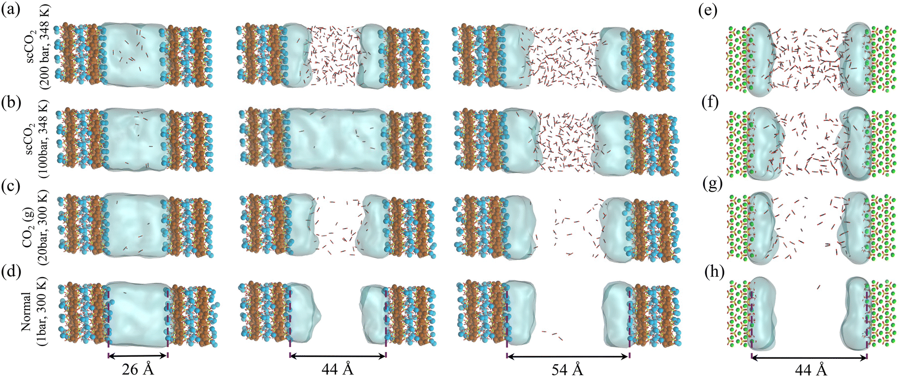Fig. 1 Competitive adsorption of H₂O–CO₂ mixtures in the slit C–S–H and forsterite porosity at normal, gaseous, and supercritical conditions. (a–d) Snapshots from the equilibrated two-phase GCMC adsorption simulations in C–S–H slit pores at different pore sizes and thermodynamic conditions. (e–h) Snapshots from equilibrated two-phase GCMC adsorption simulations in forsterite slit pores at different thermodynamic conditions. Blue and brown spheres represent intralayer and interlayer calcium in C–S–H, respectively. Green sphere represents magnesium. Silicate chains are depicted in yellow-red sticks. The continuous light blue cloud represents water and CO₂ is shown by black and red sticks.

In the temperature and pressure ranges considered here, CO₂ could only penetrate the slit pore when the interlayer distance is more than 30 Å, while the interfacial water remains on the surface regardless of the distance, Fig. 2. Moreover, the total number of adsorbed water molecules converges to an asymptotic value at large pore sizes (>40 Å), as shown by the dashed line in Fig. 2. The number of adsorbed water molecules per volume on the surface of forsterite is, in general, lower than that on the surface of C–S–H, again showing the more hydrophilic surface of C–S–H than forsterite. Also, at the largest slit-pore distance (54 Å for C–S–H and 44 Å for forsterite), we observe that the number of adsorbed water molecules on the surface of forsterite/C–S–H at 200 bar and 348 K is lower compared to those at 100 bar and 348 K. Similar observations can be made for simulations at 300 K. Therefore, we can conclude that CO₂ pressure can affect the amount of water adsorbed on the surface. It is also noteworthy that at interlayer distances of less than 20 Å, the density of capillary water is found to be higher than its bulk value (1 g cm⁻³), consistent with the simulations on the confined nature of water in C–S–H,^73,74 see ESI† Fig. S4.

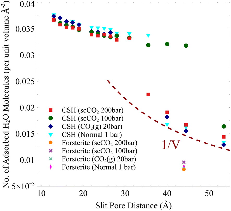Fig. 2 Number of adsorbed H₂O molecules per unit volume based on the slit-pore distance. 1/V dashed line shows that the number of adsorbed water molecules is constant beyond a certain slit pore.

To gain a more quantitative picture of the phase behavior, the resultant CO₂ mole fractions are overlaid on the experimental and theoretical bulk mixture phase diagrams^75,76 in Fig. 3. The CO₂ molar fractions corresponding to H₂O-rich and CO₂-rich are respectively shown in Fig. 3a and b. Here, we show that the CO₂ mole fraction in the slit-pore of C–S–H and forsterite with the size of less than 5 nm deviates from its bulk counterpart denoted by dashed lines in Fig. 3a and b. Also, although all GCMC simulations are initialized at CO₂-rich conditions, the equilibrium nanoconfined fluid in pores smaller than ∼30 Å turns H₂O-rich, as shown in Fig. 3a. The exact slit pore size at which CO₂-rich fluid shifts to H₂O-rich fluid depends on CO₂ pressure, temperature, and surface chemistry, among others. The observed deviation of CO₂ mole fraction from bulk values and the transition from CO₂-rich to H₂O-rich fluid in the confined space can be related to the hydrophilic nature of forsterite⁴⁹ and C–S–H (ref. 46) surfaces and the effect of surface forces in nanoscale confinements on the fluid phase behavior.^26,27 Beyond 30 Å, CO₂ permeates within the slit pores, and the mixture composition shifts toward the bulk CO₂-rich mixture (akin to the wet CO₂-rich reservoirs), as shown in Fig. 3b. The observed confinement effect has implications, especially for multi-scale porous rocks such as C–S–H, which should be taken into account in continuum models and pore-scale models.^77–79

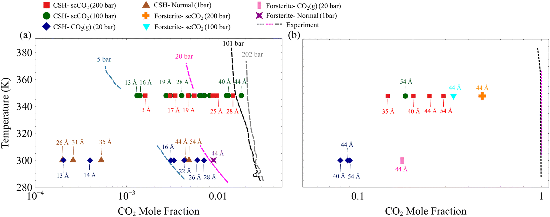Fig. 3 The H₂O–CO₂ phase coexistence diagram overlaid with the adsorbed mixture composition in the slit nano-porosities under various thermodynamic conditions computed via GCMC simulations. Dashed lines represent experimental and theoretical curves for the bulk mixture.^75,76 (a) Phase diagrams for H₂O–rich water–CO₂ mixtures. (b) CO₂–rich water–CO₂ mixtures. The CO₂ mole fractions in the slit-pore of C–S–H and forsterite derived from GCMC simulations are consistently lower than their bulk counterparts.

Determining the thickness of the adsorbed water film on the surface of metal silicate minerals is critical as it is a first-order control for carbon mineralization rates and mechanisms but is difficult to probe experimentally. Table 2 is a compilation of water film thickness data from several experiments and our adsorption simulation results. As shown in this table, experiments and simulations show adsorbed water film with thicknesses in the nanometer range. According to our GCMC adsorption simulations, the average water film thickness on the forsterite surface is 0.6–0.8 nm, depending on the temperature and pressure of the simulation. They are in good agreement with experimental values, especially those reported in recent years, such as Exp_7, Exp_8, Exp_9, and Exp_12 in Table 2. Nevertheless, we observe slight variability in the average film thickness on the surface at different carbonation conditions. To address the variability of water film thickness based on CO₂ pressure, a better picture could be achieved by calculating the distribution of species at variable carbonation conditions.

Table 2 The thickness of adsorbed water film on forsterite and C–S–H calculated via GCMC simulations and experiments

Forsterite study	Experiment/simulation	Pressure (bar)	Temperature (K)	Relative humidity (%)	Reported water film thickness on forsterite (nm)
a Molar concentration of water determined using Beer's law in FTIR setup. b Measured by IR titration using H2O. c Measured by IR titration using D2O. d Calculated in this work via Grand Canonical Monte Carlo simulations.
Loring et al. (2011)^57	Exp_1	182	323	136	2^a
Loring et al. (2011)^57	Exp_2	182	323	95	1^a
Loring et al. (2011)^57	Exp_3	182	323	81	0.1^a
Thompson et al. (2014)^56,93	Exp_4	100	308	93	1.9^a
Loring et al. (2015)^58,92	Exp_5	90	323	77	1.48^b
Loring et al. (2019)^59	Exp_6	90	323	77	1.71^b
Miller et al. (2019)^59,61	Exp_7	90	323	83	0.57^b
Miller et al. (2019)^59,61	Exp_8	90	323	84	0.66^b
Miller et al. (2019)^59,61	Exp_9	90	323	85	0.62^b
Miller et al. (2019)^59,61	Exp_10	90	323	83	0.57^c
Miller et al. (2019)^59,61	Exp_11	90	323	85	0.52^c
Placencia-Gómez et al. (2020)^54	Exp_12	90	323	85	1^b
Kerisit et al. (2021)^62,86	Exp_13	90	323	65	0.23^b
This work	Sim_1	200	348	90	0.7^d
This work	Sim_2	100	348	90	0.8^d
This work	Sim_3	20	300	90	0.6^d
This work	Sim_4	1	300	90	0.8^d

---

C–S–H study	Experiment/simulation	Pressure (bar)	Temperature (K)	Relative humidity (%)	Reported water film thickness on C–S–H surface (nm)
This work	Sim_5	200	348	90	1.3^d
This work	Sim_6	100	348	90	1.4^d
This work	Sim_7	20	300	90	1.25^d
This work	Sim_8	1	300	90	1.25^d

---

The water film thickness on the surface of C–S–H is higher than that on the hydroxylated surface of forsterite, as shown in Table 2. To clarify the latter point, we calculate the water adsorption energies for different numbers of water monolayers on both surfaces. The water adsorption energies for 1, 2, 3, and 4 monolayers of water on the {010} hydroxylated surface of forsterite and C–S–H are shown in Fig. 4. The water adsorption energies on the surface of C–S–H are shown to be consistently lower than that of the hydroxylated surface of forsterite. B3LYP calculations on gas phase clusters⁸⁰ show that the hydration energies of Mg²⁺ cation are generally lower than that of Ca²⁺. However, AIMD simulations⁵² show that calcio-olivine (γ-Ca₂SiO₄), a crystalline calcium silicate structure, is more hydrophilic than forsterite when ½ monolayer to 2 monolayers of water is adsorbed on the surface. C–S–H is more disordered and has more defects than calcio-olivine, which could entail an even higher affinity to water.

Fig. 4 The calculated water adsorption energies on C–S–H and forsterite surfaces. Calorimetry measurements⁸¹ and previous classical MD simulation results⁴⁹ on non-hydroxylated surface of forsterite are also presented for comparison.

For comparison, the adsorption energies derived from calorimetry measurements⁸¹ and previous MD simulations on the non-hydroxylated {010} surface of forsterite⁴⁹ are also included in Fig. 4. Our calculations overestimate the adsorption energies on the hydroxylated surface of forsterite by about 2–3 kcal mol⁻¹ compared to the upper values of calorimetry experiments. This slight discrepancy could be potentially due to the forcefield artifacts or an indication that not all silicate groups dissociate water molecules adjacent to the surface. We should also emphasize that using the same forcefield, Kerisit et al.⁴⁹ derive lower adsorption energy for associative adsorption of a single water monolayer on the non-hydroxylated surface of forsterite compared to experiments.

We also note that the water surface coverage for the first monolayer of hydroxylated forsterite and C–S–H is lower than that on the non-hydroxylated forsterite surface, Fig. 4. We can attribute this to the surface structure of these solids where dissociated water molecules are initially added to the surface resulting in the hydration of silicate groups and the presence of hydroxyl groups adjacent to metal cations. Therefore, the water surface coverage in hydroxylated structures with two monolayers is equivalent to one monolayer on the non-hydroxylated surface.

In addition, we calculate the adsorption energies of forsterite surface with the SPC/Fw water model,⁸² which is a modification of the SPC model with flexible bonds and angle, compared to the SPC/E water model that was originally incorporated in the modified ClayFF⁴⁹ for the surface of forsterite. As pointed out in the methods section, our GCMC calculations are performed with the SPC water model, which has different oxygen and hydrogen charges than SPC/E, and, therefore, a different dipole moment. We use the SPC model in our GCMC calculations because it predicts water vapor pressure more accurately than SPC/E.⁸³ Nevertheless, upon our calculation of water adsorption energies on the surface forsterite, SPC/Fw water model only slightly overestimates the adsorption energies compared to the SPC/E model, as shown in Fig. 4.

To resolve the spatial distribution of CO₂ and H₂O molecules and surface hydroxyl groups in the slit pore, we perform MD on fully equilibrated confined GCMC simulations. The details of these simulations are presented in the Methods section. The quantitative spatial distribution of water, CO₂, and hydroxyl groups are presented in Fig. 5. The formation of nanometer-thick interfacial water layers is evident from distributions, acting as a barrier for CO₂ molecules to contact the surface directly. Regardless of thermodynamic conditions, we observe four peaks in the water number density distributions on the surface of forsterite, see Fig. 5a–d. However, the furthest peak from the surface does not represent a fully formed water layer. This is consistent with a recent scCO₂-forsterite experiment,⁶¹ which shows 3.5 water monolayers form on the forsterite surface at 85% relative humidity. On the other hand, we also observe water layers formed on the surface of C–S–H at all pore sizes, see Fig. 5e–h. However, the appearance of multiple peaks close to each other makes it hard to distinguish water monolayers, although the overall water film thickness on C–S–H is higher than that on forsterites. These irregularities of the water density peaks on the surface of C–S–H could partly result from the observation that surface calcium atoms are more labile and less attached to the surface than surface magnesium on forsterite. This enables the water molecules to penetrate the C–S–H gel and attach to the second calcium layer and silicate groups, as shown in Fig. 5e–h. Another reason for this irregularity on the C–S–H surface is a more disordered layering of calcium ions that attract water molecules and the defects and nanoscale cavities resulting from defective silicate chains. Therefore, hydrogen bonds form between water molecules, hydroxides, and hydrated silicates that are scattered at different elevations from the surface. The heterogeneity of hydrogen bonds in the disordered C–S–H structure has been studied through simulations and experiments.^73,74,84,85

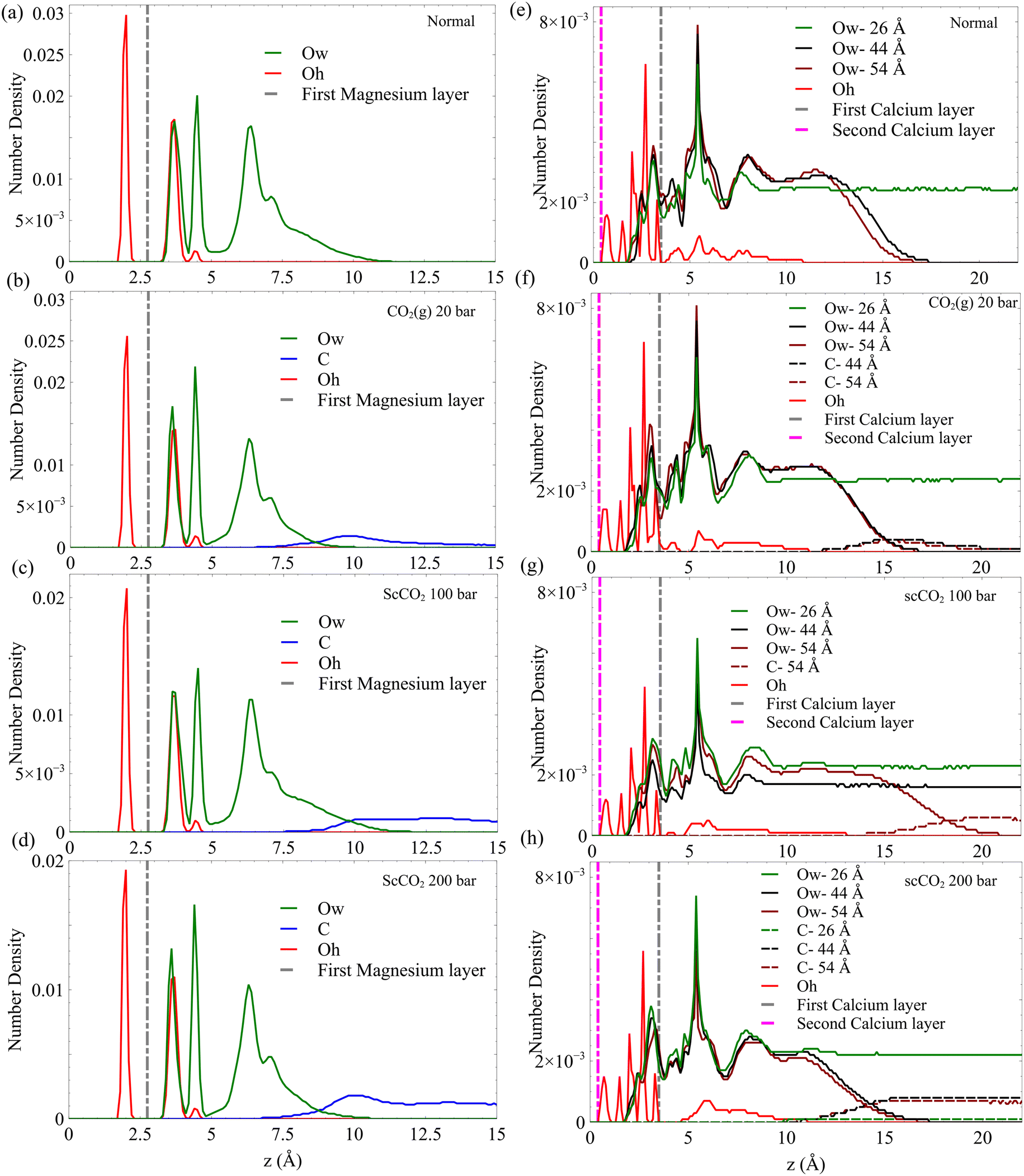Fig. 5 The average distribution of H₂O, CO₂, and OH-species in the slit-pore of forsterite and C–S–H. (a–d) Distribution of species in the slit-pore of forsterite at normal, CO₂(g), scCO₂ (100 bar), scCO₂ (200 bar), respectively. (e–h) Distribution of species in the slit-pore of C–S–H at normal, sbCO₂, scCO₂ (100 bar), scCO₂ (200 bar), respectively. The average location of the first magnesium layer on the surface of forsterite, as well as the location of the first and second calcium layers on C–S–H surface are shown by vertical dashed lines. Ow, C, and Oh represent water oxygen, carbon in carbon dioxide, and surface hydroxide oxygen, respectively.

The formation of hydration layers has been previously reported for both forsterite⁴⁹ and C–S–H (ref. 51) in unsaturated and saturated conditions, respectively. Additionally, recent Fast Force Mapping (FFM) experiments on the surface of boehmite⁸⁶ illustrate the formation of the first water layer on the surface cavities (here, the silicate groups) and the second layer forming on top of hydroxide groups. This is consistent with our results on the surface of forsterite, as shown in Fig. 5a–d. For the surface of C–S–H, which is much more disordered, the appearance of multiple water density peaks around the surface demonstrates the same phenomena, as shown in Fig. 5e–h.

Another significant aspect of the distribution diagrams is that upon the entrance of the dense CO₂ inside the pore, the last water layer contracts, and CO₂ distribution peaks at the interface, as could be seen by comparing the distribution at ambient (1 bar) gaseous to supercritical CO₂ (100, 200 bar) in Fig. 5. Although the number of water layers does not change, this could be a sign that CO₂ pressure, if above a certain threshold, might alter the number of water layers. The appearance of interfacial peaks in CO₂ distribution at all four conditions is a characteristic of immiscible mixtures verified through experiments and simulations.^87–90 However, after juxtaposing water distributions with those of carbon dioxide, we confirm that although CO₂ is not a good solvent for dipolar water, the appearance of overlapping shoulders between two species is indicative of enhanced mutual solubility at the interface. This is attributed to the interfacial capillary wave phenomenon and the Coulombic attraction between H₂O and CO₂ molecules.²⁰ This could potentially amplify the rate of CO₂ speciation at the interface. Another important feature of the resulted distributions is that the proximity of CO₂ and hydroxides within the nanolayered hydration films, especially on the surface of C–S–H, may increase the bicarbonate and carbonate production rate. Although it is well established from previous simulations that the thin water film on hydrophilic material displaces CO₂ away from the surface, this proximity of CO₂ molecules and surface hydroxides motivates us to explore the energetics of CO₂ physisorption on the surface.

Energetics of CO₂ speciation on metal silicate surfaces

Our adsorption simulations are non-reactive. Thus, it is critical to resolve the mechanistic picture of CO₂ speciation in adsorbed water nanofilms. CO₂ may speciate to carbonic acid and bicarbonate within the nanofilm in the presence of dissolved cations.⁶¹ Moreover, it is probable that CO₂ reacts with surface hydroxyl groups and surface cations. However, since CO₂ molecules are displaced from the surface due to the presence of the adsorbed water film, it is necessary to quantify the free energy required to bring CO₂ close to the surface. Since the residence time of water molecules around solvated Mg²⁺ ion is in the order of microseconds,⁴⁷ the water coordination number around surface Mg²⁺ cations is important. Therefore, to sample the full phase space in our free energy calculation for the adsorption of CO₂ on the forsterite surface, we consider the surface Mg water coordination number in addition to the perpendicular distance of CO₂ from the surface. The coordination number is defined as: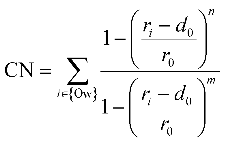where r_ij is the distance of water molecule i with the surface Mg, r₀ is set to 1 Å, d₀ is set to 2.2 Å, n is equal to 4, and m is equal to 8. The value of d₀ is taken from the peak distance of the surface Mg–water pair distribution function.

The resulting two-dimensional free energy landscape is shown in Fig. 6a. The minimum energy path (MEP) of the CO₂ molecule as it goes from the solution to the vicinity of the surface is calculated via the Nudged Elastic Band technique (NEB) method.⁹¹ As shown in the figure, the coordination number of surface Mg changes from two to one as CO₂ approaches the surface. Also, depending on the initial location of the CO₂ molecule, three distinct MEPs are derived for the cases where CO₂ is initially located at the 2nd, 3rd, and 4th layers of the adsorbed water, as shown in Fig. 6a. However, the energy that is required for the CO₂ molecule to pass through the layers and reach the surface is not affected by the initial position of the CO₂. This perhaps shows that regardless of the number of adsorbed water layers, which depends on the relative humidity and CO₂ pressure, the energy of CO₂ physisorption on the forsterite surface is unique. Also, the calculated free energy of CO₂ adsorption is 2.5 kcal mol⁻¹ higher than the adsorption free energy previously calculated by Kerisit et al.⁴⁹ for the non-hydroxylated {010} surface of forsterite. However, the magnesium coordination number was not considered in the PMF calculation in that work. Therefore, this energy difference could either be the consequence of incorporating magnesium coordination number, the existence of a stronger hydrogen bond structure due to surface hydroxides, or the difference in computational methods used.

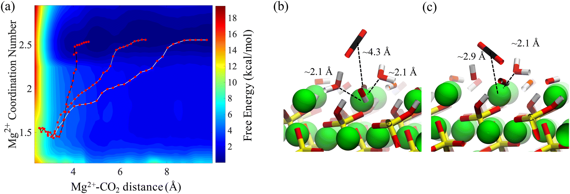Fig. 6 Potential-of-Mean-Force (PMF) for the adsorption of CO₂ from the solution on the surface of forsterite. (a) 2D PMF for the adsorption CO₂ on the surface. The three red-dotted paths represent minimum free energy paths corresponding to CO₂ adsorption from the edge of the 2nd, 3rd and 4th adsorbed water layer. While these three paths are distinct, they show that Mg²⁺ dehydration is necessary for the adsorption of CO₂ on the forsterite surfaces. Surface magnesium and the adsorbed CO₂ molecule with (b) two and (c) one neighboring water molecule. Free energy calculations show the departure of one water molecule is thermodynamically necessary for CO₂ adsorption.

It is noteworthy that although we calculate the free energy of CO₂ adsorption on the surface in contact with bulk water, it was previously shown that the structure of the water layers is not drastically different when the forsterite surface is in contact with a various number of water monolayers and supercritical CO₂.⁴⁹ These findings are consistent with in situ XRD measurements of H₂O–CO₂ sorption in hydrophilic montmorillonite,^92,93 where CO₂ intercalation was found limited when the hydration level goes beyond one water layer, regardless of isomorphous Me²⁺ exchange.

We also calculate the associative adsorption of CO₂ at random surface sites of C–S–H, as shown in Fig. 7. We find that, like the forsterite case, CO₂ is more stable in the solution than adsorbed on the surface. However, a metastable state is observed when the CO₂ molecule and surface Ca²⁺ ions are separated by about 3.2 Å on the C–S–H surface. As shown in the inset, the oxygen of the CO₂ molecule in the metastable state is oriented toward the surface calcium cation, reminiscent of a weakly chemisorbed state.⁹⁴ Unlike the forsterite case where no minimum is observed, this unique characteristic of the C–S–H surface urges us to consider interfacial CO₂ reactions.

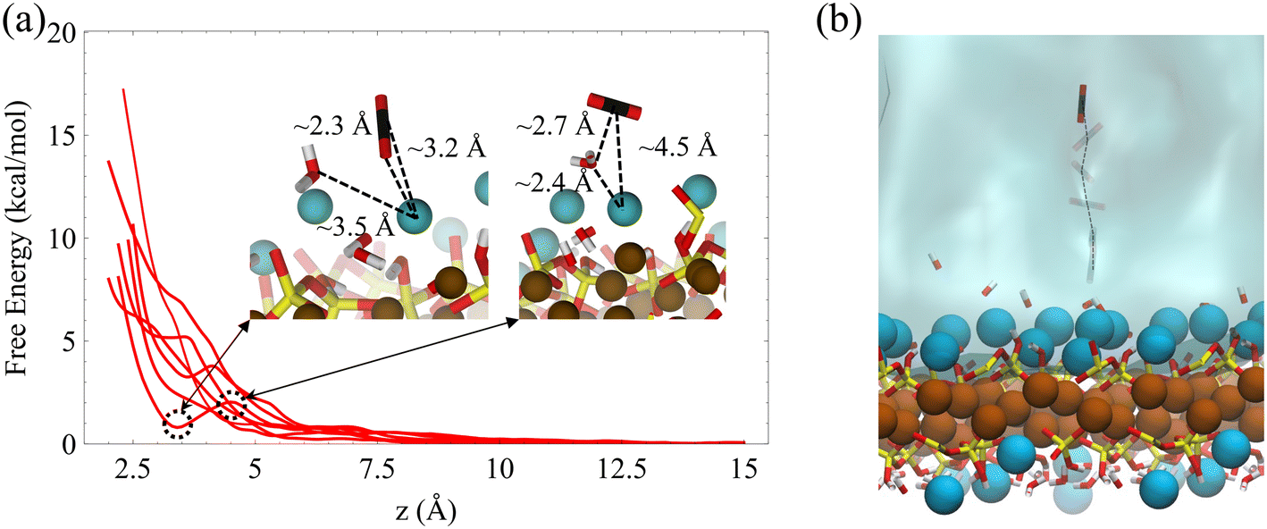Fig. 7 Non-reactive interaction of CO₂ molecule with wet C–S–H. (a) Physisorption of a CO₂ molecule on the surface of C–S–H. Multiple free energy curves are derived for random surface calcium atoms. The insets demonstrate a CO₂ molecule on the surface at the metastable state and the transition state. (b) The umbrella sampling stages for the adsorption of CO₂ on the surface.

For the carbonation progression, the physisorbed CO₂ must speciate to carbonic acid and bicarbonate by reacting with interfacial water molecules or surface-bound hydroxide. Here, we use Density Functional Theory (DFT) along with the Nudged Elastic Band (NEB) method to calculate the corresponding reaction paths, see the Methods section. Fig. 8a summarizes the three reaction paths. The adsorbed, transition, intermediate, and product states are schematically shown for each reaction path in Fig. 8b–e.

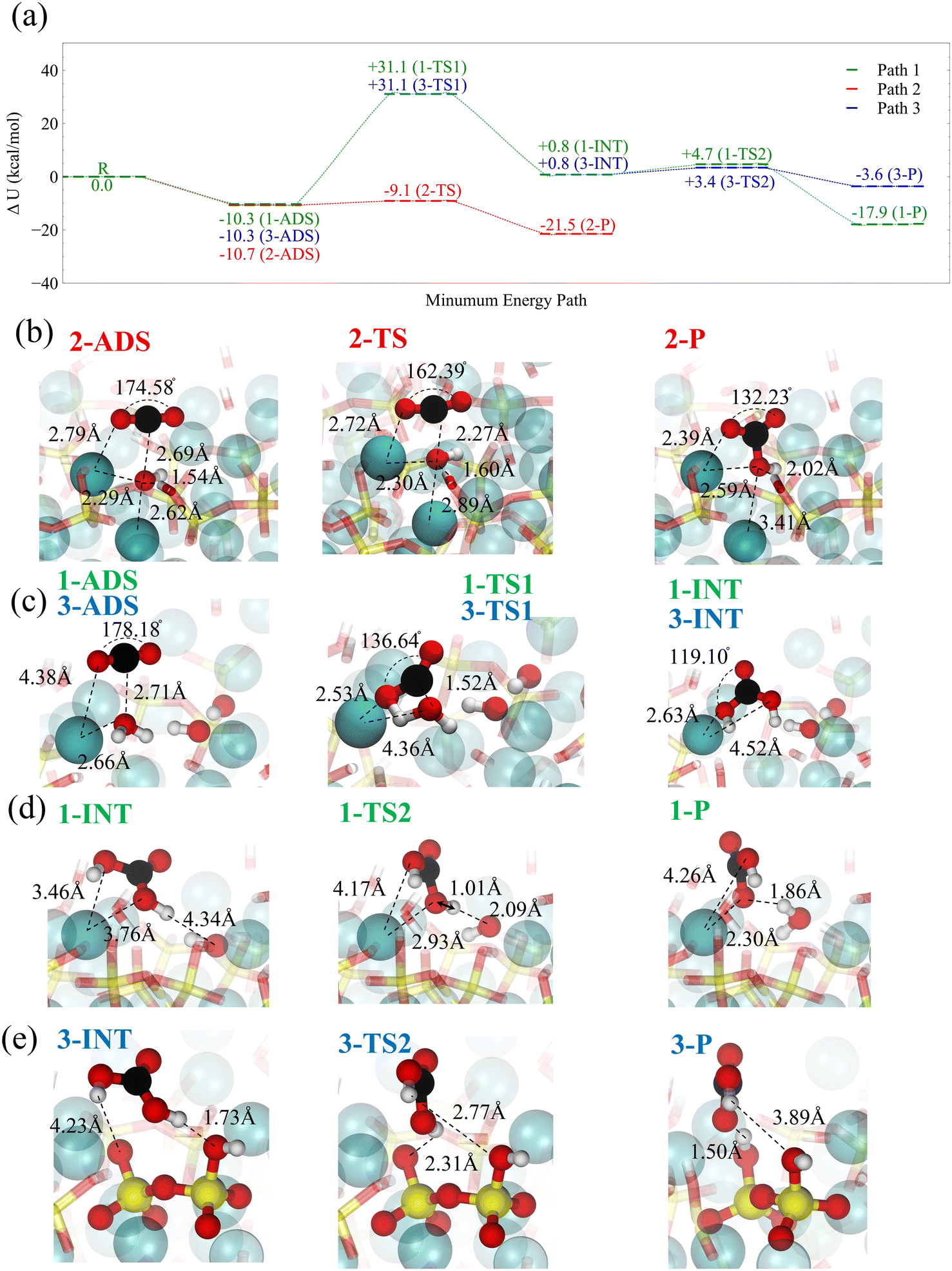Fig. 8 Reactive interaction of CO₂ molecule with wet C–S–H. (a) DFT calculation of the reaction pathways between CO₂ and C–S–H. (Path 1) The reaction between CO₂ and bound water at the hydroxide site. (Path 2) The reaction between CO₂ and surface-bound hydroxide. Strong physisorption is followed by a chemical reaction with a low barrier leading to the formation of bicarbonate. (Path 3) The reaction between CO₂ and bound water at the dangling oxygen site. (b) Snapshots of the adsorbed state (ADS), transition state (TS) and product (P) for reaction paths 2. (c) Snapshots of the ADS, TS and intermediate (INT) state for the reaction of surface water and CO₂ in path 1 and 3. d) Snapshots of the dissociation of carbonic acid to bicarbonate through reaction with surface hydroxide. e) Snapshots of the dissociation of carbonic acid to bicarbonate through reaction with dangling oxygen in silicates.

The most significant reaction occurs at the hydroxide site (path 2), where strong physisorption is connected to a chemical reaction by a low barrier, leading to the formation of bicarbonate, see Fig. 8b. In a fully hydrated environment, it takes about 3–10 kcal mol⁻¹ to bring CO₂ to the hydroxide site on the surface of C–S–H, see Fig. 7a. The overall energy barrier associated with this path is lower than or in the same range of the free energy barrier for bicarbonate formation in solutions as calculated via ab initio MD.⁹⁵ However, the abundance of hydroxide sites on the surface of C–S–H considerably impacts the overall rate of bicarbonate formation when compared to solution reactions. On the other hand, the reaction barrier of CO₂ with water, according to paths 2 and 3, if seen from the adsorbate, is approximately 10 kcal mol⁻¹ lower than the corresponding gas-phase reaction.^96,97 The snapshots of this reaction are shown in Fig. 8c. Although our DFT simulations do not explicitly consider interfacial water molecules, these remarks indicate the catalytic role of the C–S–H surface. Furthermore, it should be noted that adding liquid water would further lower the barrier down to 19 kcal mol⁻¹, according to coupled-cluster theory CCSD(T) calculations,⁹⁶ without taking to account any surface catalytic effects. Once carbonic acid forms, it can dissociate, either transferring a proton to a neighboring unhydrated dangling silicate dimer oxygen on the C–S–H surface (path 3) or a neighboring hydroxide (path 1), see Fig. 8d and e. With a wetted surface, the first option for proton transfer is unlikely, and the proton transfer to hydroxide is far more exothermic. In both paths 1 and 3, the adsorbed CO₂ reacts with surface water and forms carbonic acid in a concerted reaction.

It is noteworthy that ab initio molecular dynamics (AIMD) simulations in bulk aqueous water show that CO₂ could react with water to form bicarbonate and a hydronium ion, followed by the formation of carbonic acid in a stepwise reaction.⁹⁸ Similar routes for this reaction could be imagined to happen in the adsorbed water nanofilm on C–S–H and forsterite, leading to the formation of bicarbonate followed by the structural migration of excess proton to the surface hydroxide. Whether through reaction path 2 or in the adsorbed water nanofilm, the formation of bicarbonate is confirmed experimentally through in situ¹H–¹³C Cross-Polarized NMR spectroscopy on forsterite nanoparticles.⁶¹ However, bicarbonates were not found on fused silica surfaces. As we demonstrated earlier in this work, it is energetically unlikely to bring CO₂ to the surface of forsterite in the presence of surface water layers. Therefore, by ruling out the formation of carbonic acid through the direct reaction of CO₂ with the surface hydroxide or surface water, there remain two possible reaction pathways: the reaction of CO₂ with water 1) in the solvation shell of dissolved magnesium in the thin water film,⁶¹ or 2) at the interface of dense CO₂ and water nanofilm. However, for the further progression of carbonation reaction to carbonate nucleation, whether on the C–S–H or forsterite, the carbonic acid needs to turn into bicarbonate and carbonate. The specific mechanisms for these deprotonation reactions are still not clear. We delve into the mechanistic picture of these reactions in a future paper.

Methods

Grand canonical Monte Carlo simulations. Two-phase adsorption simulations in the present study, namely bulk mixture and slit pore adsorption studies were carried out using the Grand Canonical Monte Carlo (GCMC) simulation approach. Towhee package⁹⁹ was utilized to perform all the Monte Carlo simulations in the grand canonical ensemble (μ_H2Oμ_CO2VT) using the Configurational Biased Monte Carlo (CBMC) technique.¹⁰⁰ The configurational-biased insertion or deletion or reinsertion probabilities are 0.25 and 0.125 for water and CO₂, respectively. The biased molecular translation probabilities are 0.75 and 0.375 for water and CO₂ with a maximum displacement of 0.5 Å. The biased molecular rotation probability is 0.5 for all molecules with the maximum rotation of 0.05 rad. Details of the bulk mixture adsorption simulations are provided in ESI† Note S1 and Fig. S1–S3. The confined CO₂–H₂O adsorption simulations are carried out between two C–S–H and forsterite slabs with dimensions of 26 Å × 23 Å and 26 Å × 26 Å, respectively. Due to high computational costs, layers are fixed in these simulations. Such an assumption has a negligible effect on the adsorption properties in non-swelling systems such as hardened concrete and igneous rocks. We used the conventional SPC water model,¹⁰¹ EPM2 CO₂ model,¹⁰² and Lorentz–Berthelot combination rule to model CO₂–H₂O mixtures. Such a combination might slightly underestimate the interfacial tension between water and carbon dioxide.¹⁷ However, this would not significantly alter the thickness of interfacial water films that are governed by the water–mineral interfacial tension. ClayFF¹⁰³ and its modified version⁴⁹ are used respectively to model C–S–H and forsterite surfaces. We apply Lorentz–Berthelot mixing rules to describe solid–fluid interactions. While the Lorentz–Berthelot mixing rule overestimates the single water adsorption energy on forsterite by ∼10% (ΔE_cal = −31 kcal mol⁻¹vs. ΔE_LBmixing = −34 kcal mol⁻¹), it matches the adsorption energy measured via calorimetry at three mono-layers water coverage.⁴⁹ Therefore, the mixing rule satisfactorily predicts adsorption properties at thermodynamic conditions relevant to this work (RH ∼90%). However, a reparameterization of the modified ClayFF potential would warrant a better match with experiments and DFT calculations at lower relative humidity levels (water coverage below two monolayers). In contrast to ClayFF, variable charges for the C–S–H constituents were employed, similar to the previous simulation work on C–S–H,¹⁰⁴ to ensure charge-neutrality. Before GCMC calculations, C–S–H layers are relaxed in the MD simulations with the CSH-FF potential, a version of ClayFF tuned specifically to model C–S–H structures and reproduce its mechanical properties. Similarly, MD relaxation is done for the hydroxylated {010} surface of forsterite using the modified Clay-FF potential. Forsterite surface was terminated at M2 sites recognized as the most stable termination through X-ray reflectivity,¹⁰⁵ DFT,⁵² and molecular simulations.^106,107 MD simulations are done in the NVT ensemble using the Nosé–Hoover thermostat with a relaxation time of 100 steps and a timestep of 1 fs. The adsorption process in the slit pore was performed at four different thermodynamic conditions represented in Table 1. All confined GCMC simulations are equilibrated with at least 25 million Monte Carlo (MC) steps. We continued slow converging simulations up to 60 million steps to ensure proper convergence.

Molecular dynamics simulations. MD simulations are performed in the canonical ensemble (NVT) with Nosé–Hoover thermostat and a time step of 1 fs using LAMMPS software.¹⁰⁸ We use the same potentials as in GCMC calculations except for C–S–H, where flexible SPC water model¹⁰⁹ and flexible EPM2 model for CO₂ molecules¹¹⁰ were used. Also, the SPC/E water model was used for forsterite, consistent with Kerisit et al.⁴⁹ We allowed the first two layers of the surface to vibrate freely and kept the rest of the atoms in the substrate fixed to reduce the computational cost and for to enable the inner layers as a bulk-like structure. The cell is equilibrated for 100 ps, and the distribution analysis is derived from a production phase of 10 ns.

Potential-of-mean-force (PMF) calculations. The energetics of the physisorption and dissociation of respectively carbon dioxide and metal on the solid surface is determined via the umbrella sampling (US) technique as implemented in the “PLUMED 2.5” add-on package to LAMMPS.¹¹¹ Here, we use a biased harmonic spring with a stiffness of 200 kcal mol⁻¹ Å⁻² and 120 kcal mol⁻¹ Å⁻² between the object (CO₂ molecule for the case of adsorption, Me²⁺ cation for the case of dissociation) and a reference Me²⁺ atom on the surface respectively. The normal distance to the solid surface is taken as the “collective variable”, and sampling windows are separated by 0.1 Å. CSH-FF¹¹² and a modified version of Clay-FF⁵² were used as forcefields for the adsorption of CO₂ on the surface of CSH and forsterite, respectively. An additional collective variable, the surface Mg water coordination number, is also considered, as discussed in the main text. The harmonic spring with a stiffness of 2000 kcal mol⁻¹ is chosen for the coordination number. Histograms of the distribution of the collective variables were produced after 500 ps of equilibration phase, and another 1 ns of the production phase of MD runs at 300 K in the NVT ensemble. The substrate (except the first two layers) was fixed. A weak harmonic potential was also considered in the ‘xy’ plane (parallel to the surface) to keep the CO₂ molecule in the desired adsorption/desorption site, enclosed in a cylinder with the fixed reference atoms on its base. The free energy difference is then obtained via the weighted histogram analysis method (WHAM).¹¹³

Density functional theory calculations. A double layer of C–S–H with cell lengths a × b × c = 26.54 Å × 24.44 Å × 18.20 Å and cell angle γ = 82.5° and the other angles 90° has been created with a Ca/Si ratio of 1.7 as described in ref. 104. For stabilization, two layers of water were added to the lower surface. A single CO₂ molecule was placed 10 Å above the unwetted surface to obtain a reference structure for unreacted CO₂. The entire structure was pre-optimized using ReaxFF¹⁰⁴ as implemented in LAMMPS. First, an MD was run with a 0.25 fs time step, and a ramp brought up the temperature from 1 K to 298.15 K within 100 ps. Next, the MD was allowed to run for 500 ps before the ensemble was cooled down to 1 K within 500 ps. This yields a realistic initial guess structure for DFT calculations, with all chemically reasonable re-combinations and dissociations of water molecules completed. To obtain starting structures for adsorption and chemically reacted products, the CO₂ molecule had been shifted 3 Å and 1 Å above each reactive site, respectively. Reactive sites were 1) water on the surface 2) hydroxide on the surface, 3) an unhydrated dangling oxygen in a silicate dimer. This setup had been proven reasonable in a previous investigation.¹¹⁴ The starting structures were then also pre-optimized as described above.

For all DFT calculations, the program CP2K¹¹⁵ has been used with a combined Gaussian and plane waves ansatz. A double-ζ polarized basis set optimized for condensed phase¹¹⁶ was applied with a cutoff value of 500 Ry for the plane waves basis and GTH pseudopotentials.^117–119 The Kohn–Sham equations were solved to an accuracy of 10⁻⁶ E_h with the revised PBE^120,121 GGA functional and the D3 set of dispersion corrections.¹²² Extensive benchmark calculations show that revised PBE GGA functional with D3 dispersion correction is among the top performers in GGA functionals.^123,124 The pre-optimized structures were fully optimized without any constraints, and the resulting structures were interpolated for NEB calculations. First, the NEB was optimized within the D-NEB¹²⁵ framework until a maximum error of 5 mE_h a₀⁻¹ in RMS gradients and 10⁻² a₀ in RMS displacement had been achieved. Next, the band optimization continued using IT-NEB¹²⁶ for 10 steps before it switched to CI-NEB¹²⁷ until the final convergence of 0.5 mE_h a₀⁻¹ in RMS gradients and 10⁻³ a₀ in RMS displacements had been achieved, which corresponds to an accuracy of at least 1 kJ mol⁻¹. Minima were converged to at least 0.45 mE_h a₀⁻¹ maximum gradient and 0.003 a₀ maximum displacements. We note that the direct calculation of eigenvalues through the diagonalization of the Hessian matrix is imperative to confirm the transition state obtained vis the NEB method. In the case of NEB calculations in this work, the number of plane waves is very high in our DFT calculations to the level that the calculation of the Hessian matrix becomes impractical.

Competing interests

The authors declare no competing interests.

Conflicts of interest

There are no conflicts to declare.

Acknowledgements

This material is based on work supported by the U.S. Department of Energy (DOE), Office of Science, Office of Basic Energy Sciences (BES), Chemical Sciences, Geosciences, and Biosciences Division through its Geosciences program at the University of California Irvine through an Early Career award to MJAQ (DE-SC0022301) and at Pacific Northwest National Laboratory (PNNL). Any opinions, findings, conclusions, or recommendations expressed in this material are those of the authors and do not necessarily reflect those of the funding agency. We also thank Dr. Russell Detwiler for fruitful discussions.

References

1. J. M. Matter and P. B. Kelemen, Nat. Geosci., 2009, 2, 837–841.
2. S. K. White, F. A. Spane, H. T. Schaef, Q. R. S. Miller, M. D. White, J. A. Horner and B. P. McGrail, Environ. Sci. Technol., 2020, 54, 14609–14616.
3. S. R. Gislason and E. H. Oelkers, Science, 2014, 344, 373–374.
4. M. F. Bertos, S. J. R. Simons, C. D. Hills and P. J. Carey, J. Hazard. Mater., 2004, 112, 193–205.
5. B. P. McGrail, H. T. Schaef, A. M. Ho, Y.-J. Chien, J. J. Dooley and C. L. Davidson, J. Geophys. Res.: Solid Earth, 2006, 111(B12) DOI:10.1029/2005JB004169.
6. D. S. Goldberg, T. Takahashi and A. L. Slagle, Proc. Natl. Acad. Sci. U. S. A., 2008, 105, 9920–9925.
7. D. S. Goldberg, D. V. Kent and P. E. Olsen, Proc. Natl. Acad. Sci. U. S. A., 2010, 107, 1327–1332.
8. C. Marieni, T. J. Henstock and D. A. H. Teagle, Geophys. Res. Lett., 2013, 40, 6219–6224.
9. S. Ó. Snæbjörnsdóttir, F. Wiese, T. Fridriksson, H. Ármansson, G. M. Einarsson and S. R. Gislason, Energy Procedia, 2014, 63, 4585–4600.
10. I. M. Power, J. McCutcheon, A. L. Harrison, S. A. Wilson, G. M. Dipple, S. Kelly, C. Southam and G. Southam, Minerals, 2014, 4, 399–436.
11. S. A. Wilson, A. L. Harrison, G. M. Dipple, I. M. Power, S. L. L. Barker, K. Ulrich Mayer, S. J. Fallon, M. Raudsepp and G. Southam, Int. J. Greenhouse Gas Control, 2014, 25, 121–140.
12. D. N. Huntzinger, J. S. Gierke, L. L. Sutter, S. K. Kawatra and T. C. Eisele, J. Hazard. Mater., 2009, 168, 31–37.
13. J. K. Stolaroff, G. V. Lowry and D. W. Keith, Energy Convers. Manage., 2005, 46, 687–699.
14. G. Rim, N. Roy, D. Zhao, S. Kawashima, P. Stallworth, S. G. Greenbaum and A.-H. A. Park, Faraday Discuss., 2021, 230, 187–212.
15. W. K. O'Connor, D. C. Dahlin, G. E. Rush, C. L. Dahlin and W. K. Collins, Min. Metall. Explor., 2002, 19, 95–101.
16. National Academies of Sciences, Engineering, and Medicine, Negative Emissions Technologies and Reliable Sequestration: A Research Agenda, 2018.
17. I. C. Bourg, L. E. Beckingham and D. J. DePaolo, Environ. Sci. Technol., 2015, 49, 10265–10284.
18. J. Alcalde, S. Flude, M. Wilkinson, G. Johnson, K. Edlmann, C. E. Bond, V. Scott, S. M. V. Gilfillan, X. Ogaya and R. S. Haszeldine, Nat. Commun., 2018, 9, 2201.
19. L. D. Gelb, K. E. Gubbins, R. Radhakrishnan and M. Sliwinska-Bartkowiak, Rep. Prog. Phys., 1999, 62, 1573–1659.
20. B. K. Peterson, J. P. R. B. Walton and K. E. Gubbins, J. Chem. Soc., Faraday Trans. 2, 1986, 82, 1789–1800.
21. E. E. Santiso, A. M. George, M. Sliwinska-bartkowiak, M. B. Nardelli and K. E. Gubbins, Adsorption, 2005, 1, 349–354.
22. N. Chakraborty, Z. Karpyn, S. Liu, H. Yoon and T. Dewers, J. Nat. Gas Sci. Eng., 2020, 76, 103120.
23. A. Cihan, T. K. Tokunaga and J. T. Birkholzer, Langmuir, 2019, 35, 9611–9621.
24. T. K. Tokunaga, W. Shen, J. Wan, Y. Kim, A. Cihan, Y. Zhang and S. Finsterle, Water Resour. Res., 2017, 53, 9757–9770.
25. A. Erfani, K. Szutkowski, C. P. Aichele and J. L. White, Langmuir, 2021, 37, 858–866.
26. O. Vincent, B. Marguet and A. D. Stroock, Langmuir, 2017, 33, 1655–1661.
27. A. Cihan, T. K. Tokunaga and J. T. Birkholzer, Water Resour. Res., 2021, 57, e2021WR029720.
28. H. Li, E. Fratini, W.-S. Chiang, P. Baglioni, E. Mamontov and S.-H. Chen, Phys. Rev. E: Stat., Nonlinear, Soft Matter Phys., 2012, 86, 061505.
29. R. Velasco, M. Pathak, P. Panja and M. Deo, in Unconventional Resources Technology Conference, Austin, Texas, 24–26 July 2017, Society of Exploration Geophysicists, American Association of Petroleum Geologists, Society of Petroleum Engineers, 2017, pp. 3248–3257.
30. K. Wu, Z. Chen, J. Li, X. Li, J. Xu and X. Dong, Proc. Natl. Acad. Sci. U. S. A., 2017, 114, 3358–3363.
31. P. Chiquet, D. Broseta and S. Thibeau, Geofluids, 2007, 7, 112–122.
32. E. A. Al-Khdheeawi, S. Vialle, A. Barifcani, M. Sarmadivaleh and S. Iglauer, Int. J. Greenhouse Gas Control, 2018, 68, 216–229.
33. S. Iglauer, C. H. Pentland and A. Busch, Water Resour. Res., 2015, 51, 729–774.
34. S. Iglauer and A. Al-Yaseri, Adv. Geo-Energy Res., 2021, 5, 347–350.
35. M. J. Abdolhosseini Qomi, K. J. Krakowiak, M. Bauchy, K. L. Stewart, R. Shahsavari, D. Jagannathan, D. B. Brommer, A. Baronnet, M. J. Buehler, S. Yip, F.-J. Ulm, K. J. Van Vliet and R. J.-M. Pellenq, Nat. Commun., 2014, 5, 4960.
36. M. Bauchy, B. Wang, M. Wang, Y. Yu, M. J. Abdolhosseini Qomi, M. M. Smedskjaer, C. Bichara, F.-J. Ulm and R. Pellenq, Acta Mater., 2016, 121, 234–239.
37. A. Morshedifard, S. Masoumi and M. J. Abdolhosseini Qomi, Nat. Commun., 2018, 9, 1785.
38. F. Xi, S. J. Davis, P. Ciais, D. Crawford-Brown, D. Guan, C. Pade, T. Shi, M. Syddall, J. Lv, L. Ji, L. Bing, J. Wang, W. Wei, K.-H. Yang, B. Lagerblad, I. Galan, C. Andrade, Y. Zhang and Z. Liu, Nat. Geosci., 2016, 9, 880–883.
39. T. A. Boden, R. J. Andres and G. Marland, Global, Regional, and National Fossil-Fuel CO2 Emissions (1751–2010) (V. 2013), Environmental System Science Data Infrastructure for a Virtual Ecosystem; Carbon Dioxide Information Analysis Center (CDIAC), Oak Ridge National Laboratory (ORNL), Oak Ridge, TN (United States), 2013.
40. L. Barcelo, J. Kline, G. Walenta and E. Gartner, Mater. Struct., 2014, 47, 1055–1065.
41. G. Rimmelé, V. Barlet-Gouédard, O. Porcherie, B. Goffé and F. Brunet, Cem. Concr. Res., 2008, 38, 1038–1048.
42. V. Barlet-Gouédard, G. Rimmelé, O. Porcherie, N. Quisel and J. Desroches, Int. J. Greenhouse Gas Control, 2009, 3, 206–216.
43. E. A. C. Panduro, M. Torsæter, K. Gawel, R. Bjørge, A. Gibaud, Y. Yang, S. Bruns, Y. Zheng, H. O. Sørensen and D. W. Breiby, Environ. Sci. Technol., 2017, 51, 9344–9351.
44. P. Renforth, Nat. Commun., 2019, 10, 1401.
45. P. J. M. Monteiro, G. Geng, D. Marchon, J. Li, P. Alapati, K. E. Kurtis and M. J. Abdolhosseini Qomi, Cem. Concr. Res., 2019, 124, 105806.
46. M. J. Abdolhosseini Qomi, M. Bauchy, F.-J. Ulm and R. J.-M. Pellenq, J. Chem. Phys., 2014, 140, 054515.
47. H. Erras-Hanauer, T. Clark and R. van Eldik, Coord. Chem. Rev., 2003, 238–239, 233–253.
48. M. J. Abdolhosseini Qomi, Q. R. S. Miller, S. Zare, H. T. Schaef, J. P. Kaszuba and K. M. Rosso, Nat. Rev. Chem., 2022 DOI:10.1038/s41570-022-00418-1.
49. S. Kerisit, J. H. Weare and A. R. Felmy, Geochim. Cosmochim. Acta, 2012, 84, 137–151.
50. A. Botan, B. Rotenberg, V. Marry, P. Turq and B. Noetinger, J. Phys. Chem. C, 2010, 114, 14962–14969.
51. S. Masoumi, S. Zare, H. Valipour and M. J. Abdolhosseini Qomi, J. Phys. Chem. C, 2019, 123, 4755–4766.
52. S. Kerisit, E. J. Bylaska and A. R. Felmy, Chem. Geol., 2013, 359, 81–89.
53. Q. R. S. Miller, J. P. Kaszuba, S. N. Kerisit, H. T. Schaef, M. E. Bowden, B. Peter McGrail and K. M. Rosso, Environ. Sci.: Nano, 2020, 7, 1068–1081.
54. E. Placencia-Gómez, S. N. Kerisit, H. S. Mehta, O. Qafoku, C. J. Thompson, T. R. Graham, E. S. Ilton and J. S. Loring, Environ. Sci. Technol., 2020, 54, 6888–6899.
55. C. J. Thompson, J. S. Loring, K. M. Rosso and Z. Wang, Int. J. Greenhouse Gas Control, 2013, 18, 246–255.
56. C. J. Thompson, P. F. Martin, J. Chen, P. Benezeth, H. T. Schaef, K. M. Rosso, A. R. Felmy and J. S. Loring, Rev. Sci. Instrum., 2014, 85, 044102.
57. J. S. Loring, C. J. Thompson, Z. Wang, A. G. Joly, D. S. Sklarew, H. T. Schaef, E. S. Ilton, K. M. Rosso and A. R. Felmy, Environ. Sci. Technol., 2011, 45, 6204–6210.
58. J. S. Loring, J. Chen, P. Bénézeth, O. Qafoku, E. S. Ilton, N. M. Washton, C. J. Thompson, P. F. Martin, B. P. McGrail, K. M. Rosso, A. R. Felmy and H. T. Schaef, Langmuir, 2015, 31, 7533–7543.
59. J. S. Loring, Q. R. S. Miller, C. J. Thompson and H. T. Schaef, in Science of Carbon Storage in Deep Saline Formations, ed. P. Newell and A. G. Ilgen, Elsevier, 2019, pp. 63–88.
60. X. Zhang, A. S. Lea, A. M. Chaka, J. S. Loring, S. T. Mergelsberg, E. Nakouzi, O. Qafoku, J. J. De Yoreo, H. T. Schaef and K. M. Rosso, Nat. Mater., 2021, 1–7.
61. Q. R. S. Miller, D. A. Dixon, S. D. Burton, E. D. Walter, D. W. Hoyt, A. S. McNeill, J. D. Moon, K. S. Thanthiriwatte, E. S. Ilton, O. Qafoku, C. J. Thompson, H. T. Schaef, K. M. Rosso and J. S. Loring, J. Phys. Chem. C, 2019, 123, 12871–12885.
62. S. N. Kerisit, S. T. Mergelsberg, C. J. Thompson, S. K. White and J. S. Loring, Environ. Sci. Technol., 2021, 55, 12539–12548.
63. S. T. Mergelsberg, S. N. Kerisit, E. S. Ilton, O. Qafoku, C. J. Thompson and J. S. Loring, Chem. Commun., 2020, 56, 12154–12157.
64. R. S. Smith, Z. Li, Z. Dohnálek and B. D. Kay, J. Phys. Chem. C, 2014, 118, 29091–29100.
65. S. A. Hamid, Z. Kristallogr., 1981, 154, 189–198.
66. S. Peuble, M. Andreani, P. Gouze, M. Pollet-Villard, B. Reynard and B. Van de Moortele, Chem. Geol., 2018, 476, 150–160.
67. K. Marquardt and U. H. Faul, Phys. Chem. Miner., 2018, 45, 139–172.
68. T. Xing, W. Zhu, F. Fusseis and H. Lisabeth, Solid Earth, 2018, 9, 879–896.
69. S. Erdmann, B. Scaillet, C. Martel and A. Cadoux, J. Petrol., 2014, 55, 2377–2402.
70. A. J. Luhmann, B. M. Tutolo, B. C. Bagley, D. F. R. Mildner, W. E. Seyfried Jr. and M. O. Saar, Water Resour. Res., 2017, 53, 1908–1927.
71. A. Silvestri, E. Ataman, A. Budi, S. L. S. Stipp, J. D. Gale and P. Raiteri, Langmuir, 2019, 35, 16669–16678.
72. A. Silvestri, A. Budi, E. Ataman, M. H. M. Olsson, M. P. Andersson, S. L. S. Stipp, J. D. Gale and P. Raiteri, J. Phys. Chem. C, 2017, 121, 24025–24035.
73. M. J. Abdolhosseini Qomi, M. Bauchy, F.-J. Ulm and R. J.-M. Pellenq, J. Chem. Phys., 2014, 140, 054515.
74. M. Youssef, R. J.-M. Pellenq and B. Yildiz, J. Am. Chem. Soc., 2011, 133, 2499–2510.
75. N. Spycher, K. Pruess and J. Ennis-King, Geochim. Cosmochim. Acta, 2003, 67, 3015–3031.
76. L. W. Diamond and N. N. Akinfiev, Fluid Phase Equilib., 2003, 208, 265–290.
77. Q. Li, C. I. Steefel and Y.-S. Jun, Environ. Sci. Technol., 2017, 51, 10861–10871.
78. G. W. Scherer and B. Huet, Int. J. Greenhouse Gas Control, 2009, 3, 731–735.
79. A. Raoof, H. M. Nick, T. K. T. Wolterbeek and C. J. Spiers, Int. J. Greenhouse Gas Control, 2012, 11, S67–S77.
80. M. Pavlov, P. E. M. Siegbahn and M. Sandström, J. Phys. Chem. A, 1998, 102, 219–228.
81. S. Chen and A. Navrotsky, Am. Mineral., 2010, 95, 112–117.
82. Y. Wu, H. L. Tepper and G. A. Voth, J. Chem. Phys., 2006, 124, 024503.
83. J. Vorholz, V. I. Harismiadis, B. Rumpf, A. Z. Panagiotopoulos and G. Maurer, Fluid Phase Equilib., 2000, 170, 203–234.
84. D. Hou, H. Ma, Y. Zhu and Z. Li, Acta Mater., 2014, 67, 81–94.
85. B. Li, N. Li, H. J. H. Brouwers, Q. Yu and W. Chen, Constr. Build. Mater., 2020, 233, 117347.
86. E. Nakouzi, A. G. Stack, S. Kerisit, B. A. Legg, C. J. Mundy, G. K. Schenter, J. Chun and J. J. De Yoreo, J. Phys. Chem. C, 2021, 125, 1282–1291.
87. S. R. P. da Rocha, K. P. Johnston, R. E. Westacott and P. J. Rossky, J. Phys. Chem. B, 2001, 105, 12092–12104.
88. B. Kvamme, A. Graue, T. Buanes, T. Kuznetsova and G. Ersland, Int. J. Greenhouse Gas Control, 2007, 1, 236–246.
89. T. Kuznetsova and B. Kvamme, Phys. Chem. Chem. Phys., 2002, 4, 937–941.
90. D. N. Espinoza and J. C. Santamarina, Water Resour. Res., 2011, 15, 707–719.
91. H. Jónsson, G. Mills and K. W. Jacobsen, in Classical and Quantum Dynamics in Condensed Phase Simulations, World Scientific, 1998, pp. 385–404.
92. H. T. Schaef, J. S. Loring, V.-A. Glezakou, Q. R. S. Miller, J. Chen, A. T. Owen, M.-S. Lee, E. S. Ilton, A. R. Felmy, B. P. McGrail and C. J. Thompson, Geochim. Cosmochim. Acta, 2015, 161, 248–257.
93. J. S. Loring, E. S. Ilton, J. Chen, C. J. Thompson, P. F. Martin, P. Bénézeth, K. M. Rosso, A. R. Felmy and H. T. Schaef, Langmuir, 2014, 30, 6120–6128.
94. U. Burghaus, Prog. Surf. Sci., 2014, 89, 161–217.
95. A. Stirling, J. Phys. Chem. B, 2011, 115, 14683–14687.
96. M. T. Nguyen, M. H. Matus, V. E. Jackson, V. T. Ngan, J. R. Rustad and D. A. Dixon, J. Phys. Chem. A, 2008, 112, 10386–10398.
97. S. Yamabe and N. Kawagishi, Theor. Chem. Acc., 2011, 130, 909–918.
98. A. Stirling and I. Pápai, J. Phys. Chem. B, 2010, 114, 16854–16859.
99. M. G. Martin, MCCCS Towhee: a tool for Monte Carlo molecular simulation, Mol. Simul., 2013, 39, 1212–1222 , (accessed 29 September 2018).
100. G. C. A. M. Mooij, D. Frenkel and B. Smit, J. Phys.: Condens. Matter, 1992, 4, L255.
101. H. J. C. Berendsen, J. P. M. Postma, W. F. van Gunsteren and J. Hermans, in Intermolecular Forces: Proceedings of the Fourteenth Jerusalem Symposium on Quantum Chemistry and Biochemistry Held in Jerusalem, Israel, April 13–16, 1981, ed. B. Pullman, Springer Netherlands, Dordrecht, 1981, pp. 331–342.
102. J. G. Harris and K. H. Yung, J. Phys. Chem., 1995, 99, 12021–12024.
103. R. T. Cygan, J.-J. Liang and A. G. Kalinichev, J. Phys. Chem. B, 2004, 108, 1255–1266.
104. M. J. Abdolhosseini Qomi, K. J. Krakowiak, M. Bauchy, K. L. Stewart, R. Shahsavari, D. Jagannathan, D. B. Brommer, A. Baronnet, M. J. Buehler, S. Yip, F.-J. Ulm, K. J. V. Vliet and R. J.-M. Pellenq, Nat. Commun., 2014, 5, 4960.
105. H. Yan, C. Park, G. Ahn, S. Hong, D. T. Keane, C. Kenney-Benson, P. Chow, Y. Xiao and G. Shen, Geochim. Cosmochim. Acta, 2014, 145, 268–280.
106. H. E. King, M. Stimpfl, P. Deymier, M. J. Drake, C. R. A. Catlow, A. Putnis and N. H. de Leeuw, Earth Planet. Sci. Lett., 2010, 300, 11–18.
107. N. H. de Leeuw, S. C. Parker, C. R. A. Catlow and G. D. Price, Phys. Chem. Miner., 2000, 27, 332–341.
108. S. Plimpton, J. Comput. Phys., 1995, 117, 1–19.
109. H. J. C. Berendsen, J. R. Grigera and T. P. Straatsma, J. Phys. Chem., 1987, 91, 6269–6271.
110. R. T. Cygan, V. N. Romanov and E. M. Myshakin, J. Phys. Chem. C, 2012, 116, 13079–13091.
111. G. A. Tribello, M. Bonomi, D. Branduardi, C. Camilloni and G. Bussi, Comput. Phys. Commun., 2014, 185, 604–613.
112. R. Shahsavari, R. J.-M. Pellenq and F.-J. Ulm, Phys. Chem. Chem. Phys., 2011, 13, 1002–1011.
113. S. Kumar, J. M. Rosenberg, D. Bouzida, R. H. Swendsen and P. A. Kollman, J. Comput. Chem., 1992, 13, 1011–1021.
114. A. Funk and H. F. R. Trettin, Ind. Eng. Chem. Res., 2013, 52, 2168–2173.
115. R. Car and M. Parrinello, Phys. Rev. Lett., 1985, 55, 2471–2474.
116. J. VandeVondele and J. Hutter, J. Chem. Phys., 2007, 127, 114105.
117. S. Goedecker, M. Teter and J. Hutter, Phys. Rev. B: Condens. Matter Mater. Phys., 1996, 54, 1703–1710.
118. C. Hartwigsen, S. Goedecker and J. Hutter, Phys. Rev. B: Condens. Matter Mater. Phys., 1998, 58, 3641–3662.
119. M. Krack, Theor. Chem. Acc., 2005, 114, 145–152.
120. J. P. Perdew, K. Burke and M. Ernzerhof, Phys. Rev. Lett., 1996, 77, 3865–3868.
121. Y. Zhang and W. Yang, Phys. Rev. Lett., 1998, 80, 890.
122. S. Grimme, J. Antony, S. Ehrlich and H. Krieg, J. Chem. Phys., 2010, 132, 154104.
123. L. Goerigk, A. Hansen, C. Bauer, S. Ehrlich, A. Najibi and S. Grimme, Phys. Chem. Chem. Phys., 2017, 19, 32184–32215.
124. T. Gould, Phys. Chem. Chem. Phys., 2018, 20, 27735–27739.
125. S. A. Trygubenko and D. J. Wales, J. Chem. Phys., 2004, 120, 2082–2094.
126. G. Henkelman and H. Jónsson, J. Chem. Phys., 2000, 113, 9978–9985.
127. G. Henkelman, B. P. Uberuaga and H. Jónsson, J. Chem. Phys., 2000, 113, 9901–9904.

---

Footnote

† Electronic supplementary information (ESI) available. See DOI: https://doi.org/10.1039/d2en00148a

---