Modeling atmospheric aging of small-scale wood combustion emissions: distinguishing causal effects from non-causal associations

Abstract

Small-scale wood combustion is a significant source of particulate emissions. Atmospheric transformation of wood combustion emissions is a complex process involving multiple compounds interacting simultaneously. Thus, an advanced methodology is needed to study the process in order to gain a deeper understanding of the emissions. In this study, we are introducing a methodology for simplifying this complex process by detecting dependencies of observed compounds based on a measured dataset. A statistical model was fitted to describe the evolution of combustion emissions with a system of differential equations derived from the measured data. The performance of the model was evaluated using simulated and measured data showing the transformation process of small-scale wood combustion emissions. The model was able to reproduce the temporal evolution of the variables in reasonable agreement with both simulated and measured data. However, as measured emission data are complex due to multiple simultaneous interacting processes, it was not possible to conclude if all detected relationships between the variables were causal or if the variables were merely co-variant. This study provides a step toward a comprehensive, but simple, model describing the evolution of the total emissions during atmospheric aging in both gas and particle phases.

---

Environmental significance

Residential wood combustion in stoves is known as a substantial primary source of particulate matter in Europe with significant potential for secondary organic aerosol (SOA) formation during atmospheric aging. Despite numerous laboratory studies with combustion-related SOA precursors under different oxidation conditions, interactions between those conditions and aerosol constituents over the course of ageing have not been understood yet. In this study we formed a stochastic model that, based on the obtained structure of the variables and coefficients of ‘reactions’ from the measured dataset, was able to reproduce the evolution of emission in a smog chamber. Our model raises evidence for interactive processes not taken into account before with possible implications for air pollution forecasts and at-source reduction of secondary pollutant formation.

1 Introduction

Small-scale wood combustion is a common method for residential heating and has been identified as a substantial contributor to ambient levels of particulate matter in several European areas.^1–5 Wood combustion-derived aerosol, in particular from manually-fired logwood stoves, contains substantial quantities of several air pollutants, such as black carbon, polycyclic aromatic hydrocarbons (PAH), volatile organic compounds (VOC) and CO,^6,7 with consequences for Earth's radiative forcing,⁸ cloud formation,⁹ and human health.¹⁰ After their release into the atmosphere, wood combustion emissions are immediately transformed in a complex process known as “atmospheric aging” involving multiphase chemistry, leading to the oxidation and functionalization of particulate and gaseous pollutants^11,12 and the consequent formation of secondary organic and inorganic aerosol (SOA and SIA, respectively). The formation of SOA has been reported to enhance the organic aerosol concentration by a factor of two to three times the concentration of the particulate organic aerosol emitted by wood combustion, after less than 1.5 days of photochemical aging.^13–15 In addition, atmospheric aging of wood combustion emissions at nighttime has been identified as a substantial enhancer of aerosol particle concentrations.^13,16 Consequently, it has been found that atmospheric aging alters the toxicological properties of wood combustion aerosols^17,18 in addition to changing the optical properties,^19,20 with implications for the climate and human health.

Smog chambers or environmental chambers have been used to study the atmospheric transformation of single VOC or combustion emissions for several decades, offering a controlled environment and conditions similar to the atmosphere, to study the effects of, for example, the photochemical age, relative humidity, NO_x, addition of seed aerosol, oxidizing agents, etc. on emission transformation.^13,21–24 Despite several known reaction pathways from smog chamber experiments for single emission constituents or compound classes, such as PAHs,²⁵ interactions between all constituents of a real-world combustion aerosol complicate the prediction of secondary aerosol formation and its physicochemical properties.

Radicals, such as hydroxyl (OH), ozone (O₃), and nitrate (NO₃), are known to play an important role in SOA chemistry.¹¹ OH is the most important radical during photochemical aging, whereas NO₃ and O₃ are more important during dark aging.^13,26 SOA formed from photochemical and dark aging differ by chemical composition. However, both aging mechanisms are important and must be taken into account when evaluating the whole-climate implications of aging processes.²⁷ Nitrate radical chemistry is an efficient SOA formation mechanism and also an important pathway for the production of organic nitrates, serving as a NO_x sink in the atmosphere.²⁸

A few studies have been made to capture the atmospheric evolution of wood combustion emissions in both the gaseous and particulate phases.^29–32,86

Models of SOA formation and the evolution of the compounds leading to SOA can be divided into at least two groups. One group of modelling, such as the volatility basis set, aims to describe one or several features of the emission. In the volatility basis set (VBS) approach,^33,34 the evolution of the constituent phases are modeled based on the volatilities of the compounds, considering the equilibrium concentrations of different compounds in gas and particle phases and how different factors, such as chemical and physical reactions, affect the equilibrium state. This approach with the observational data from smog chamber experiments has been commonly used to estimate the SOA mass produced from combustion emission^35–40 and to estimate the proportional contributions of different SOA precursors to formed SOA.⁴¹ The VBS scheme has been also applied to model biomass-burning organic aerosol in regional chemical transport models.^42,43

The second approach to model SOA, and in particular its precursors in the gas phase, is the family of explicit chemical modeling. There exist several chemical models such as the Master Chemical Mechanism (MCM)^44,45 and GECKO-A,⁴⁶ which combine large numbers of chemical reactions and predetermined reaction coefficients to replicate the evolution of the system. The MCM has recently been applied to wood-burning emissions by running the model with the most important primary emission species to model the evolution of gas-phase species using a smaller selection of reactions from the entire system.⁴⁷ These can be used to parametrize SOA production. The Statistical Oxidation Model (SOM) offers an approach somewhere between one-quality models and explicit chemical models. The SOM uses several qualities of compounds (such as their volatility and numbers of constituent carbon and oxygen atoms) to predict the SOA mass and atomic O : C ratio.⁴⁸ The SOM has been used to simulate the formation and composition of biomass burning SOA in an environmental chamber.⁴⁹

All approaches—volatility-based, SOM, and explicit chemical modeling—are based on differential equations. These equations describe the evolution of some quantity that we are interested in modeling and can be transformed into the final product of the model. For the volatility approach, this is the volatility distribution of particles; in chemical modeling, it defines the quantities of substances in the system.

In the approaches mentioned above, the changes of gas concentrations and numbers of particles in time can be considered consequences of reactions occurring in the system. Reactions are caused by the initial compounds and certain properties of these compounds. The reaction coefficients and concentrations of initial compounds determine the rate of reactions occurring in time. Compounds can be considered causally related as those are related to each other through chemical reactions. If a reaction is favorable, initial compounds lead to an increase in products while their own concentrations decrease.

In this study, we described the connections between primary emissions and aging conditions using a causal model.⁵⁰ Models aiming to study causality are slowly being introduced to studies in atmospheric sciences, but this is the first attempt to build a causality-based model for combustion emissions. In the field of atmospheric science, causal discovery has been applied in different subfields to both test the usability of the method for a certain kind of dataset, but also to understand the causal pathways of a certain phenomenon. Examples of studies includes exploring causal networks in biosphere–atmosphere interactions,⁵¹ discovering causality in spatio-temporal datasets of surface pressures in oceans,^52,53 discovering causal pathways among atmospheric disturbances of different spatial scales in geopotential height data,⁵⁴ and testing causal discovery in synthetic atmospheric datasets of advection and diffusion.⁵⁵

The aim of this study was to evaluate whether it is possible to learn the causal relationships of variables from the system of atmospheric aging without having explicit prior information about these relations. On that account, we created a model for the complex interactions between aerosol constituents in both gaseous and particulate phases.^13,30 Here, we present the first version of our model that is able to represent dependencies between observed variables in the chamber studies in Tiitta et al. (2016)¹³ and Hartikainen et al. (2018).³⁰ In addition, we discuss the issues in data processing related to the modeling of wood combustion aging, and more generally, emission aging data sets by applying the model to artificial, simulated data sets and evaluating its accuracy.

2 Data and methods

Chamber experiments for studying the atmospheric transformation of residential wood combustion emissions were conducted in the ILMARI environmental chamber⁵⁶ at the University of Eastern Finland, as described by Tiitta et al. (2016).¹³ The particulate emissions of the dataset have been studied by Tiitta et al. (2016)¹³ and volatile emissions by Hartikainen et al. (2018).³⁰

Briefly, five chamber experiments were conducted in total using a modern heat-storing masonry heater⁵⁷ as the emission source. The masonry heater was operated with spruce logs, using both fast ignition and slow ignition for initiating the combustion experiment (detailed procedure described in Tiitta et al., 2016)¹³ to adjust the VOC-to-NO_x ratio. In each experiment, a sample of the combustion exhaust was diluted and fed into the chamber for 35 min, including the ignition, flaming combustion and residual char-burning phases of the combustion.⁵⁸ This was followed by stabilization (i.e. the period when organic compounds should reach an equilibrium state in the chamber) of the sample, after which the oxidative aging of the sample was initiated by feeding ozone into the chamber. The end of the stabilization period is treated as the starting point in our analysis. Both dark and UV-light aging experiments were conducted, representing evolution at nighttime and daytime in the atmosphere, respectively.

To investigate the daytime ambient conditions, in which OH radicals dominate the oxidative aging of emissions, we used two experiments (experiments 4B and 5B, Tiitta et al., 2016).¹³ In those, UV lights (blacklight lamps, 350 nm) were switched on immediately after feeding ozone into the chamber, and the wood combustion emission was photochemically aged for four hours. The estimated photochemical age of the sample at the end of the experiment was 0.6–0.8 days, based on the measured OH radical exposure. Two experiments were also used to investigate the nighttime evolution (experiments 2B and 3B, Tiitta et al., 2016).¹³ In those, the aging was conducted first without the UV radiation; after 4 hours of dark aging, the UV lights were switched on. The dark aging period represents nighttime ambient conditions, in which ozone and nitrate radicals dominate the oxidative aging of emissions.^13,59 The conditions in the chamber simulate polluted atmospheric boundary-layer conditions with an OH concentration of (0.5–5) × 10⁶ molecule per cm³, ozone concentrations of 20–90 ppb and NO_x concentrations of 40–120 ppb¹³ with a lower VOC-to-NO_x ratio (fast ignition: ratio ≈ 3) yielding smaller total emissions including SOA than the slow ignition cases (ratio ≈ 5).

The evolution of gases and particles in the chamber was measured by comprehensive online measurements. Gas-phase organic and inorganic compounds were measured using single gas analyzers (NO, NO₂, and O₃) and a Proton-Transfer-Reactor Time-of-Flight Mass Spectrometer (PTR-TOF-MS 8000, Ionicon Analytik, Innsbruck, Austria). The PTR-MS data set has been described in detail by Hartikainen et al. (2018).³⁰ The submicron particle size distribution was measured using a Scanning Mobility Particle Sizer (SMPS, CPC 3022, TSI) and the chemical composition and mass concentration of the particles using a Soot Particle Aerosol Mass Spectrometer (SP-HR-TOF-AMS).⁶⁰ The AMS was used to characterize the chemical signatures of particulate chemical species (organic, NO₃, SO₄, NH₄, and Chl), of which NO₃ and organic species (hereafter referred to as OA) were used as Positive Matrix Factorization (PMF) factors (POA1–2, SOA1–3, details below) in this study.

Dark and UV-induced aging were treated separately in further data analysis because the intense UV radiation affects the transformation of emissions due to photochemical reactions and further influences the dependencies between the variables. Furthermore, we had two experiments with different ignition techniques, one with fast ignition and one with slow ignition for both dark (2B and 3B) and UV light-induced aging (4B and 5B). Both experiments with the same aging type were combined into a single data set for the model.

The ignition type, which determines how fast the logwood ignites, influences the emission factors of POA and VOC emission from wood combustion, particularly those of carbonyls, aromatic hydrocarbons, and furanoic and phenolic compounds.^13,30 Hartikainen et al. (2018)³⁰ showed that during aging, furanoic and phenolic compounds decreased, while nitrogen-containing organic compounds were produced in both gaseous and particulate phases. In addition, photochemical aging especially increased the concentrations of certain gaseous carbonyls, particularly acid anhydrides.³⁰ As we combined the results of both experiments with different ignition types into a single data set, we assumed that the reactions in the chamber were similar in both data sets and that only the concentrations of the compounds differed.

2.1 Data processing

For modeling purposes, the data are needed to be harmonized and transformed into an applicable form. The SMPS provided detailed measurements of size distributions, each consisting of over 100 bins by the particle (mobility) diameter, ranging from 14.1–14.6 nm to 710.5–736.5 nm. For this study, we used a simpler representation of the size distribution, size binning of wall-loss corrected (see Section 2.3 in Tiitta et al., 2016)¹³ SMPS time series which were grouped into four larger size classes. These four classes roughly represent atmospherically relevant particle modes: under 25 nm (nucleation mode, hereafter NuclM), 25 to 100 nm (Aitken mode, AitM), 100 to 300 nm (accumulation mode, AccM), and over 300 nm (coarse mode, CoarM). Measured size bins were summed to form number concentrations of particles in four classes.

As OH radicals are one of the main oxidants in the atmospheric transformation of emission during photochemical aging, we applied OH concentration level estimation formulas (1–3) from Barmet et al. (2012)⁶¹ to calculate the OH concentration time series. The estimation was based on the d9-butanol tracer method, and the slope was determined separately for each time point from 20 observations (time period of 30 min) around the time at which the OH concentration was estimated. The reason for using only a 30-minute interval for estimating the OH at the time was that the decline of d9-butanol (hence the concentration of OH) was highly varying during the experiment. The decline in d9-butanol levels was highest right after UV lights were turned on. The slope estimation (see formula (3) in Barmet et al.⁶¹) using whole time series could have given too small estimates for the OH level right after UV lights have been turned on. Concentrations of OH that were estimated to be negative were set to zero. However, negative values were only estimated for dark aging experiments, where, according to our initial assumption, OH was not allowed to affect other variables in the model.

The applied instruments measured concentrations and size distributions with different time resolutions. PTR-MS measured every 2 seconds, whereas the SMPS scan time and sample analysis took a total of 5 minutes to conduct a single measurement. To combine variables measured by multiple measurement devices into one data set, it is important to transform data appropriately to express variables to the same time resolution. We applied simple cubic spline interpolation to interpolate SMPS data to the same time resolution as AMS data, which was 2 minutes. Data from PTR-MS and other gas analyzers were averaged over a 2 minute period.

2.1.1 Dimension reduction of PTR-MS and AMS data sets. The particle and gas phase data provided by AMS and PTR-MS, respectively, consist of mass spectra of many chemical compounds and their fragments (hereafter referred as tracers). To formulate a model that could provide a simple representation of the evolution of the emissions, we need to compress the information provided by a large number of single tracers. Thus, we aim to describe the evolution of spectra by combining tracers into a smaller number of factors with dimension reduction techniques for both gas- and particle-phase measurement (from PTR and AMS) data sets. Tracers share some properties and the underlying dependencies in the data set.

However, it is not necessarily self-evident which dimension reduction method should be applied to the data set of interest. Isokääntä et al. (2020)⁶² studied the importance of selecting the appropriate dimension reduction method to the data set in atmospheric studies. Specifically, they investigated mass spectrometer data sets acquired from chamber studies. They found that fragmentation of compounds and rapid changes in chemical composition (such as that caused by turning on UV lights) should be considered when selecting the dimension reduction technique. They suggest that for data sets in which fragmentation is usually not problematic, exploratory factor analysis (EFA) or principal component analysis (PCA) might extract those rapid changes from the data more efficiently than PMF.

We aimed to compare multiple experiments in further data analysis, and thus we applied dimension reduction techniques to the PTR-MS data sets, using all the data to form the factors instead of applying a dimension reduction method separately. For PTR-MS data, both EFA and PCA were tested, but only EFA was selected for further analysis as it provided interpretable factors. EFA was applied using the function fa from package psych⁶³ in the R environment.⁶⁴ The minimum residual technique was used for EFA and oblique Oblimin-rotation was used to enhance the separation of the tracers in each factor. In addition, tracers that had no significant contribution (i.e., loading) on any of the factors were removed from analysis, and factorization was performed again only to the remaining tracers. These removed tracers were mainly instrumental backgrounds or compounds with very small concentrations without any clear structure as a time series. Time series for the factors were calculated by the sum score method, wherein the original data are multiplied directly with the loading values from EFA, possibly with some threshold limit.⁶⁵ We selected an absolute value of 0.3 as a threshold for the loadings, meaning any loading values smaller than that were suppressed to zero before the multiplication.⁶⁶ PTR factor 2 was scaled to be positive by adding the minimum value to all the time points. Negative values were caused by the baseline correction of PTR-MS data and factorization. Factors (see Fig. 1) were identified based on their temporal evolution and identified tracers as well as their average carbon oxidation state (OS_C) contributing to each factor. For PTR-MS data, three factors were found: (1) primary VOCs, (2) photochemical aging products, and (3) dark aging products.

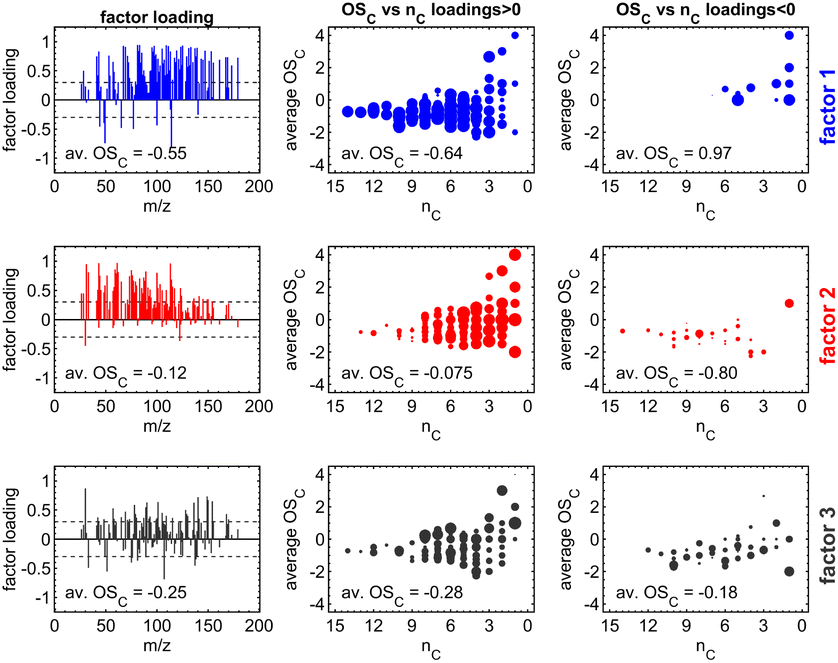Fig. 1 Illustration of the three factor loadings (in rows) from exploratory factor analysis (EFA) including the average carbon oxidation state (OS_C) for PTR-MS factors. Subplots in the left column contain the coefficients of the factor loadings and the limit of ±0.3 (dashed line), separating relevant from redundant variables. Subplots in the center (for m/z with positive factor loadings) and the right column (for m/z with negative factor loadings) visualize the OS_C dependent on the carbon number (n_C) of the detected sum formula.⁷³

PTR-MS data sets adequately identified the representative compounds (i.e., tracers that were identifiable) as a time series. It must be noted that detailed interpretation of factors would require identification for most of the compounds in the chamber, including highly oxygenated organic molecules, which was not possible with the current measurement setup.^67–70 Accurate optimization of factors is outside the scope of this study.

Factorization of the AMS data by PMF has been described in Tiitta et al. (2016)¹³ so we only summarize it here. PMF^71,72 was applied to classify the OA into five subgroups. Two factors describe the primary organic aerosol particles (POA): (1) biomass-burning OA and (2) hydrocarbon-like OA. Three factors represent the major oxidants in the formation processes of SOA: (1) formation by ozonolysis, (2) formation by nitrate/peroxy radicals, and (3) formation by OH radicals. PMF was performed using the PMF Evaluation Tool v.2.08.⁷²

2.1.2 Filtering time series. Measurements can be thought of as discrete observations from the continuous process of emission transformation. They contain measurement uncertainty, which arises from limitations of the measurement regarding the representativeness, accuracy or other factors affecting the measurement event or applied instruments. The uncertainties, referred to in the model as measurement errors, are estimated and taken into account in the filtering procedure (detailed motivation for filtering in ESI S1†).

Multiple statistical methods can be applied to estimate the state α_t of the time series from data. Instead of using all observations from the time series (smoothing), we used only observations before the estimated state (filtering). The reason for using filtering instead of smoothing was that if the model would be used to predict the evolution of the system after the end of the measurement, the information is only available until the last observation.

The filtering method was similar to locally estimated scatterplot smoothing,⁷⁴ in which observations are weighted according to the proximity of the measurement y_k,t0 from the measurement y_k,t0 which state is estimated.

w(x) = {(1 − |x|³)³}, when |x| < 1, 0, when |x| ≥ 1 (2)

We applied the method separately to every time series. The number of previous measurements used (h = time window) to estimate the current state α_k,t0 was determined in each individual time series by calculating a weighted linear regression (with coefficients β₀ and β₁ and weights w(x)) to the time series and choosing a window such that the filtered time series was representative to time series. The time series had different ratios of noise to total variation due to different measurement instruments and time resolutions. Fig. 2 shows the effect of filtering for one variable during experiment 2B.

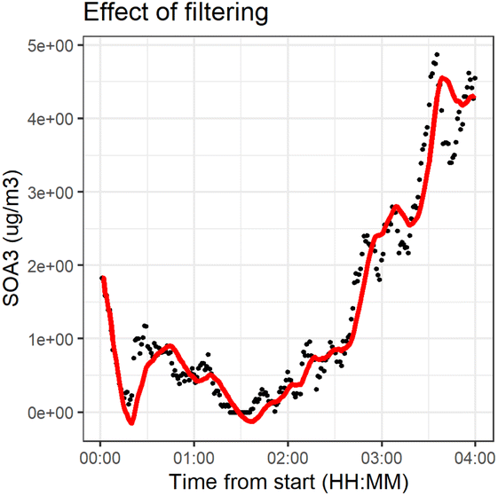Fig. 2 Effect of filtering for one variable during the dark aging period of experiment 2B. The dots represent the original measurements, and the line represents the filtered values.

2.2 Creating the model

We present a simple four-step procedure describing how the model was applied to the processed version of the emission data set. Sections 2.2.1–2.2.4 provide more detailed descriptions of selected steps in the model creation.

(1) Applying the causal discovery algorithm⁷⁵ for finding the potential causal relationships between measured variables and measured changes (Δ(x):s) in time. The algorithm returns possible causes for each measured change.

(2) Forming all possible interaction variables from measured variables such that both variables in the interaction should be potential causes suggested by the causal discovery algorithm. In addition, prior assumptions are taken into account, and thus variables with the given limitations are restricted from being considered interaction variables.

(3) Using the least absolute shrinkage and selection operator (LASSO)⁷⁶ to select predictor variables amongst interaction variables (and possible single variables suggested by the algorithm). Simultaneously, estimating the coefficients of each selected predictor using a linear model.

(4) Calculating the modeled evolution using the ordinary differential equation (ODE) system deSolve,⁷⁷ using estimated coefficients as reaction coefficients, the first observation from the experiment as the initial state and with multiple values of two parameters which the user needs to define. Select values of those parameters based on the smallest RMSE for the calculated evolution.

Sections 2.2.1–2.2.4 provide more detailed descriptions of selected steps in the model creation.

As the output of the procedure, we learn linear differential equations for each variable of interest x_j, j = 1, …, n, eqn (3):

Δ(x_j,t) = x_j,t+1 − x_j,t = β₀ + β₁x_1,t + β₂x_2,t + … + β_ikx_i,tx_k,t + … (3)

These differential equations describe how the difference of the variable value between subsequent time points is determined by values of measured variables (x_i:s describe the variables used as itself and x_ix_k variables used as interaction variables) immediately before the time interval.

2.2.1 Using a causal discovery algorithm. A causal discovery algorithm⁷⁸ attempts to find the causal structure of variables in a studied system. The causal structure refers to qualitative knowledge on the causal relations. For instance, the algorithm may indicate that X causes Y but gives no information on the strength of the effect. Fig. 3 illustrates causal graphs where one-headed arrows, called edges, tell the direction of the causality.

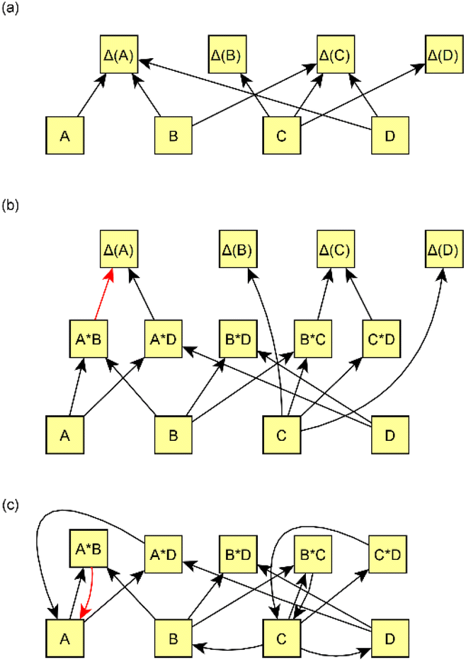Fig. 3 Examples of causal graphs and how interaction variables are formed. (a) Variables are linked to other variables by affecting Δ(x) (denoted as Δ(A) for variable A). The causal discovery algorithm searches, for each Δ(x), for the most probable variables that could have an effect. (b) The interaction variables are linked to the edges using the causal discovery algorithm. All possible interaction variables are formed based on edges in graph (a). For example, because A, B, and D all affect Δ(A), interaction variables A × B, A × D, and B × D are formed, and those are possible to affect Δ(A). In this graph, we assume that some of the interaction edges (e.g., B × D → Δ(A)) are not selected in least absolute shrinkage and selection operator (LASSO). (c) Alternative way figure (b) can be drawn as a cyclic graph. Edge from, e.g., A × B → Δ(A) in figure (b) is substituted by an edge A × B → A in figure (c). We have used (c) to represent the edges in the results section. The color of the edge is related to the direction of the effect: black indicates a positive effect and red denotes a negative effect.

Causal discovery methods can be divided into constraint-based and score-based approaches.^78,79 We applied the PC-algorithm⁷⁸ which is a constraint-based method implemented in the R package r-causal.⁷⁵ In constraint-based methods, a series of tests for (conditional) independence between the variables are carried out. Based on these tests, conclusions on the causal structure can be made. For instance, if X and Y are dependent, Z and Y are dependent, but X and Z are independent when conditioned on Y, it can be concluded that the causal graph has a V-structure X → Y ← Z. However, without auxiliary information it is possible to construct the causal graph only up to an equivalence class,⁷⁸ which in practice means the direction of some arrows may remain unknown.

The implementation of the PC-algorithm⁷⁵ has two parameters which the user needs to define, “depth” and “alpha” which are hereafter referred to as tuning parameters. Wongchokprasitti (2019)⁷⁵ explains that the depth determines “a number of nodes conditioned on in the search”. Depth values used in the algorithm were two, three, and infinite, meaning that every node can be further conditioned in the search. Alpha, which is set between zero and one, indicates the statistical significance of the dependency between searched variables. However, significance was used here as a tuning parameter to allow the number of edges to rise with larger alpha values. Alpha values of 0.01, 0.05, 0.2, and 0.3 have been used for wood combustion data sets. For simulated data sets (see Sections 3.1 and S2†) alpha values of 0.05, 0.2, and 0.3 were used. For depth, values of 3 and −1 (describing unlimited depth) were used.

The PC-algorithm was used to search for potential cause variables (sources or sinks) for each measured compound (AMS: NO₃, POA1–2, SOA1–3, SMPS: NuclM, AitM, AccM, CoarM, PTR: factors PTR1–3, gas phase: NO, NO₂, O₃, OH). A crucial part of the causal discovery algorithm is the implementation of prior knowledge. We used prior information to restrict presumably impossible or negligible dependencies. The apparent a priori difference in prior information between the two aging types is that in dark aging, OH is not allowed to affect any of the variables; however, in photochemical aging, OH can affect other variables excluding those derived from the particle size distribution. OH was also forced to affect SOA3, which was characterized as OH radical formation products in a previous study.¹³ Furthermore, the effects from size distribution variables on any other variables, POA on SOA, AMS variables on gas-phase variables, and negligible variables (those with small concentrations) on any other variable were not permitted. As the applied causal discovery algorithm is based on correlations, variables that have negligible effects on absolute concentrations could have been found to have large effects in this correlation-based search due to randomness. Allowed dependencies for causal discovery algorithm have been listed in Table 1.

Table 1 Allowed predictors for each response variable given for a causal discovery algorithm

Allowed dependencies
Response variable Δ(x)	Predictor variable
Dark aging
Size variables (NuclM, AitM, AccM, CoarseM)	Size variables (NuclM, AitM, AccM, CoarseM)
SOA1–3	SOA1–3, NO3, PTR1–3, gas-phase variables (NO, NO2, O3)
POA1–2, NO3	POA1–2, SOA1–3, NO3, PTR1–3, gas-phase variables (NO, NO2, O3)
PTR1-3, gas-phase variables (NO, NO2, O3)	PTR1-3, gas-phase variables (NO, NO2, O3)
Photochemical aging
Size variables (NuclM, AitM, AccM CoarseM)	Size variables (NuclM, AitM, AccM, CoarseM)
SOA1–3	SOA1–3, NO3, PTR1–3, gas-phase variables (NO, NO2, O3, OH)
POA1–2, NO3	POA1–2, SOA1–3, NO3, PTR1–3, gas-phase variables (NO, NO2, O3, OH)
PTR1–3, gas-phase variables (NO, NO2, O3, OH)	PTR1–3, gas-phase variables (NO, NO2, O3, OH)

---

2.2.2 Forming interaction variables. The causal discovery algorithm suggested several potential edges (i.e., directed connections) between variables which were turned into interaction variables. We used the suggestion from the discovery algorithm as a starting point to form a final structure to be used in the model. For each variable Y, the algorithm provided a list of variables X that could cause Y, X → Y. We used those variables X to form interaction variables for explaining Y.

Interaction variables predicting Y were formed by pairing potential causes of Y. Both paired variables needed to be suggested by the causal discovery algorithm. The only limitation for variables was that variable interactions were not allowed to violate prior assumptions, as explained in Section 2.2.1. For example, if it is known that Z cannot cause Y, it cannot be included in a list of interaction variables that could cause Y. In this step, we formed a list of potential interaction variables for each variable Y. Fig. 3b shows an example of the formation of interaction variables.

In addition to interaction variables, we also allowed some single variables to act as predictors. The evolution of the physical properties of particles and many chemical reactions typically involves more than, for example, just one compound or phase state, but there are exceptions. As an example, particles of the same size can coagulate during evolution and form larger particles.

Similar solutions appear in the literature. In chemical kinetics theory,⁸⁰ one or more variables react to form other compound(s). The changes in time of the produced compound's concentration can then be represented as a product of concentrations of reacting compounds multiplied by the rate coefficient and time t. Interaction variables and some single variables found by the algorithm were used to select suitable explanatory variables for the effects of variables to the response variable Δ(x).

The calculation of interaction variables may be performed directly by using all possible variables in the data set and then selecting suitable explanatory variables for each response variable from amongst all interaction variables. This can be performed by a causal discovery algorithm or some other method. However, if the number of initial (single) variables is n, then the number of possible two-variable interactions is which is large even for relatively small n. Therefore, a preselection of most potential variables to form these interaction variables reduces the number of interaction variables formed remarkably. The preselection is also justified because then we do not have clearly incorrect interaction variables in the next step (LASSO). We found out that the interaction variables can be highly correlated, therefore some clearly incorrect interaction variables could be selected, if all variables will be used for forming interaction variables.

2.2.3 Accounting for multicollinearity with LASSO. Interaction variables also give rise to some challenges for the selection of variables. Interaction variables are often highly correlated, as two interaction variables may share one common variable. Highly correlated variables can lead to multicollinearity in coefficient estimation. When data have a multicollinearity problem, coefficients of interaction variables might suffer from biases, and small changes in the model can lead to large changes in its output. Therefore, it is important to note the possibility of multicollinearity in predictors.

When interaction variables have been formed, there are usually many correlated variables that can explain each response variable Δ(x). We used LASSO regression (Bayesian approach⁸¹ based on Park & Casella, 2008 (ref. 82)) to reduce the number of variables and multicollinearity in the set of explanatory variables. LASSO shrinks the coefficients of some redundant variables to be almost or equal to zero, and thus reduces the number of effective variables. Variables with coefficients close to zero were consequently excluded from the structure. Variables that had non-zero coefficients in the LASSO fit were used as predictor variables for Δ(x)s. Coefficients of these variables were used as coefficients in the final model. Fig. 3b shows an example of the exclusion of some interaction variables after using LASSO.

Negative coefficients are only permitted when the measured value of a predicted variable is decreased due to the process, which is shown in the model as the interaction variable including the variable that is predicted itself. Without this limitation, the modeled value of a variable can fall below zero during a calculation, which is not physically realistic. If a variable with a negative coefficient does not have a predicted variable in the response variable, the model attempts to fix that by changing the predictor to one with a positive coefficient (usually negatively correlated with the original predictor) or to some interaction variable that includes the predicted variable.

2.2.4 Finding the best model and calculating the evolution based on the fit. We evaluated the model fit by calculating the evolution of the system based on the model's structure and estimated coefficients. We used the R package deSolve⁷⁷ to calculate the evolution of the modeled linear ordinary differential equation system. Selection of the best model was then performed based on that evolution. We calculated the Root Mean Squared Error (RMSE) for each variation of the tuning parameters (see Section 2.2.1 for description) and selected the model based on the smallest RMSE for the calculated evolution.

As we had only two data sets for both dark and light induced aging, we did not want to use separate data sets for training and evaluating the model fit. As the ignition type also affects, for example, the chemical composition of the emission,¹³ evolution between the data sets might not be directly comparable. Therefore, we used both ignition types for searching for the structure and estimating the coefficients of the model.

2.3 Simulation studies

In order to validate our model, we fitted it first to simulated data mimicking combustion emissions and then to real measured data from wood combustion experiments. Details about data generation and experiments can be found in ESI S2, Tables 2 and S1.† For the case where the dependencies between variables are not completely known, causal discovery algorithms offer a solution to find missing causal pathways, noncausal dependencies, and covariances. As a causal discovery algorithm attempts to search for dependencies based on data, there might be incorrect dependencies in the structure formed by an algorithm. These can be due to, for example, uncertainties in the measured concentrations of variables, which can result in an observed dependence that is weak and therefore not selected for the model.

Table 2 Datasets used in this study. Wood combustion datasets are measured datasets from the ILMARI environment (Tiitta et al., 2016). Simulated datasets are completely artificial datasets representing the evolution of differential equation systems

	Dataset	How evolution is formed
Wood combustion datasets	2B and 3B	Dark aging experiments of wood combustion emission
	4B and 5B	Photochemical aging experiments of wood combustion emission
Simulated datasets	Small	Differential equation system using mass action kinetics
	Large	Differential equation system. Independent linear differential equations for each variable. System does not follow mass action kinetics

---

The atmospheric aging process of wood combustion emissions is one such case in which we have limited prior knowledge. For the reliability of the obtained results from our experimental data sets, it is important to know how the causal discovery algorithm combined with our model would function, if we had the information regarding the correct structure resulting from the aging process (see Table S1†). Thus, we simulated a data set representing our observations with known structures and connections in order to test and validate our model for combustion measurement-type data. The details of the simulations are provided in the ESI S2.†

3 Results

As the evolution of emission is known to be different in the dark and under UV aging conditions, experiments were separated based on the aging type. In addition, prior information was defined separately for dark and UV aging experiments (see Section 2.2.1).

The causal discovery algorithm was used for both dark aging experiments (the dark aging parts of 2B and 3B) using the data from the experiments as the input for the model. Similarly, the UV aging parts of 4B and 5B were used to search the structure for UV aging. Thus, both experiments with the same aging type have the same dependence structure between variables, and the coefficients for the experiments of the same aging type were the same. After estimating the coefficients, modeled evolution of the system was then calculated and compared to the measured evolution of the experiment. The best model based on tuning parameters (alpha and depth, details in Section 2.2) was then selected. The time point zero in each experiment represents the start of the aging period. As the full graph of the model holds so many connections, it is impossible to interpret. Thus, we show here only subsets of the full graph. Magnitudes of each effect are given in Table S8† for dark aging experiments and Table S9† for photochemical aging experiments.

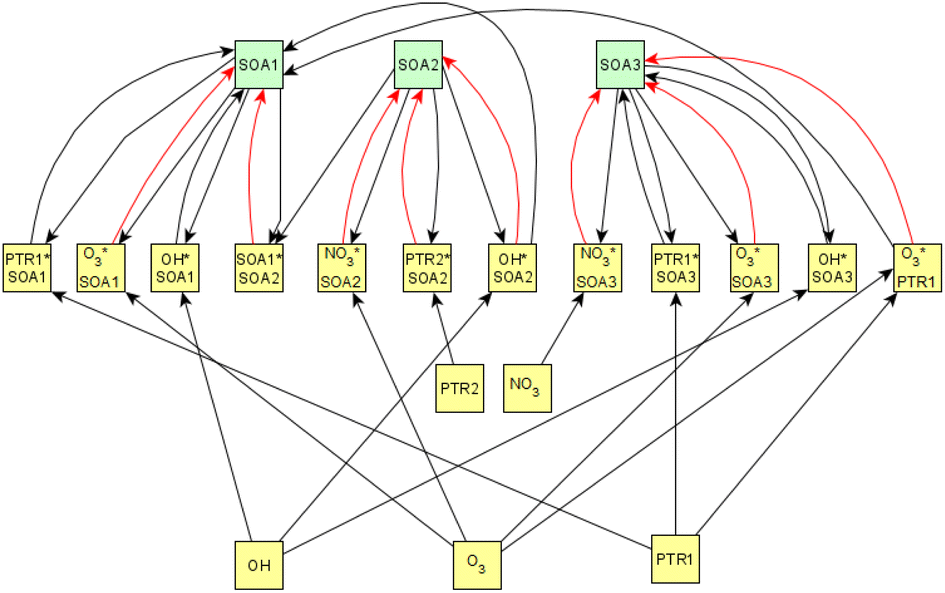
For dark aging experiments, the sub-graph of the model showing dependencies for SOA variables is shown in Fig. 4. Coefficients for the edges are provided in the ESI.† For SOA, most of the edges connected seem to be possible causes.

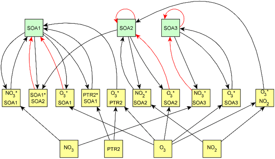Fig. 4 Secondary organic aerosol (SOA)-related part of the causal graph for dark aging experiments. SOA variables are highlighted in green. O₃ and NO₂ are measured from the gas phase, PTR2 is formed from Proton-Transfer-Reactor Time-of-Flight Mass Spectrometer (PTR-ToF-MS) measurements, and NO₃ signatured aerosol and SOA1–3 are given by particle-phase measurements with an Aerosol Mass Spectrometer (AMS). PTR2 represents photochemical aging products and SOA factors represents (1) formation by ozonolysis, (2) formation by nitrate/peroxy radicals, and (3) formation by OH radicals. The color of the arrow represents the sign of the effect, black arrows have positive coefficient and red arrows have negative.

For SOA1, the main increase of the concentration is due to the reaction with ozone (O₃ × SOA1 → SOA1). The benefit of this type of model is that the variables in the model can be act at the same time as outcomes and predictor variables for some other variable. More specifically, the current level of a variable can be the predictor for the level at the next time point. e.g. in the example of O₃ × SOA1, reactions of existing SOA1 with O₃ decrease the level of SOA1. If, in turn, SOA1 reacts with NO₃, it increases the level of SOA1.

In SOA2, organic nitrates are present which were formed through oxidation of organic emission constituents by nitrate radicals (NO₂ × SOA2 → SOA2). For SOA3, the change in concentration is minor compared to that of SOA2 during dark aging. According to the model, some increase in SOA2 and SOA3 occurs due to ozone reactions (O₃ × SOA2 → SOA2 and O₃ × SOA3 → SOA3). Based on Tiitta et al. (2016),¹³ SOA1 is formed by ozonolysis, SOA2 is formed by NO₃ and RO₃ radicals, and SOA3 is formed by OH radicals. SOA3 is mostly formed during the UV aging period; hence the edges related to SOA3 during the dark aging period are not very important.

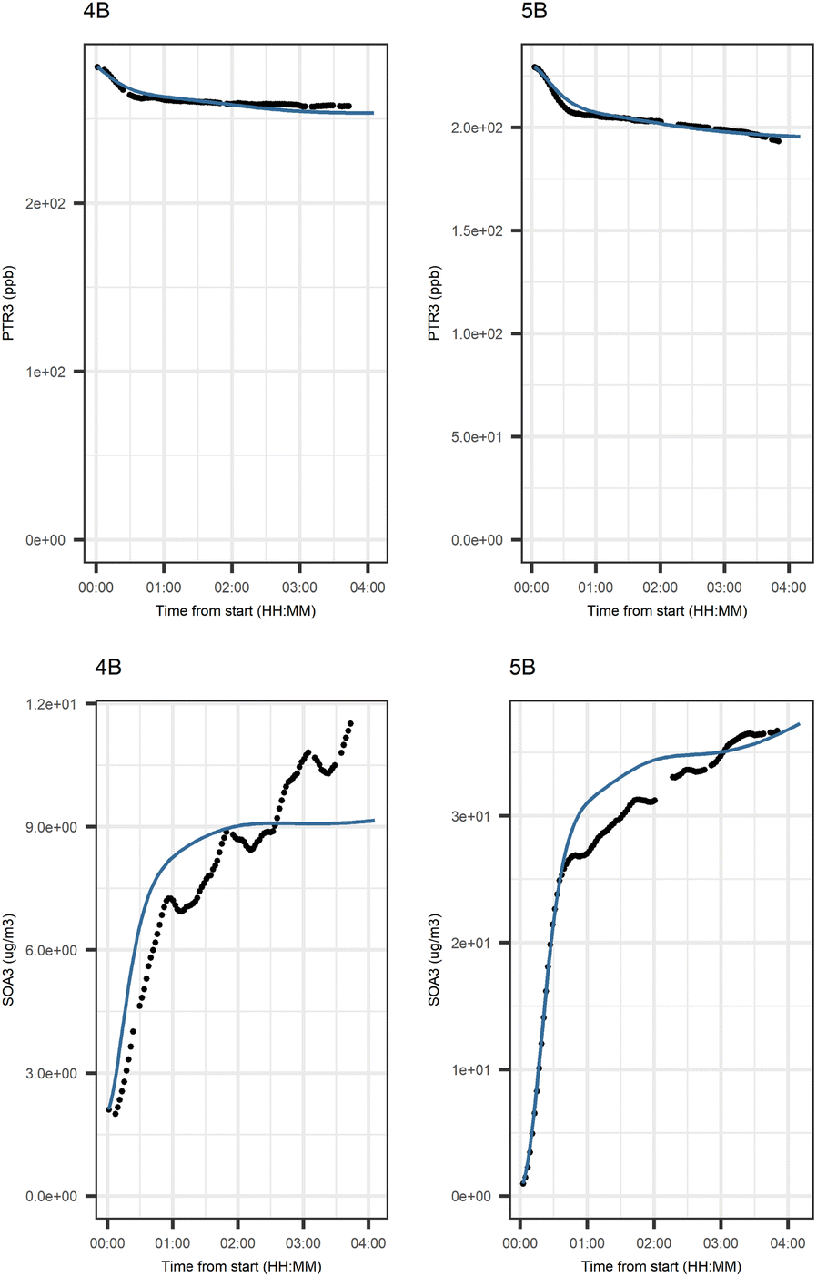
Fig. 5 shows that the evolution based on the model for both experiments follow the measured evolution well for SOA2, but for SOA1 the model was not able to accurately describe the evolution. In general, some factors (SOA1, SOA3, and PTR2) have minor differences between the measured and modeled evolutions in one or both experiments. Differences between the evolution calculated based on the Lasso approach and Jackknife resampling with OLS in e.g.Fig. 5 are most likely due to the differences in estimation methods which causes differences in estimated coefficients and hence, the modeled evolution. All coefficients for the dark aging model and figures for other variables can be found in the ESI file (Table S8 and Fig. S2–S4).†

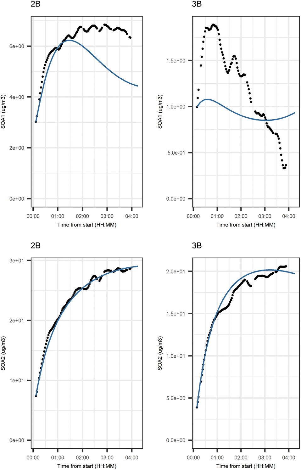Fig. 5 Evolution of secondary organic aerosol (SOA) factors 1 and 2 from Aerosol Mass Spectrometer (AMS) particle-phase measurements in dark aging experiments. SOA factors represent (1) formation by ozonolysis, and (2) formation by nitrate/peroxy radicals. Black points represent the filtered version of variable and the blue line shows the modeled evolution.

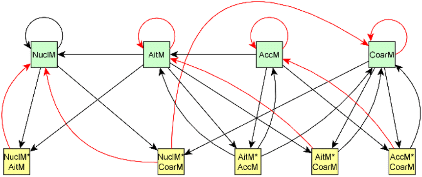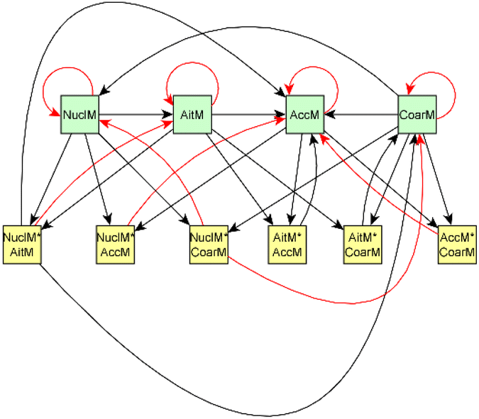
Fig. 6 Particle size related part of the causal graph for dark aging experiments. Particle-size related variables (nucleation mode (NuclM, <25 nm), Aitken mode (AitM, 25–100 nm), accumulation mode (AccM, 100–300 nm), and coarse mode (CoarseM, >300 nm)), are highlighted in green and yellow squares represent interaction variables. All variables are measured using a Scanning Mobility Particle Sizer (SMPS). The color of the arrow represents the sign of the effect; black arrows represent the positive coefficient and red arrows the negative coefficient.

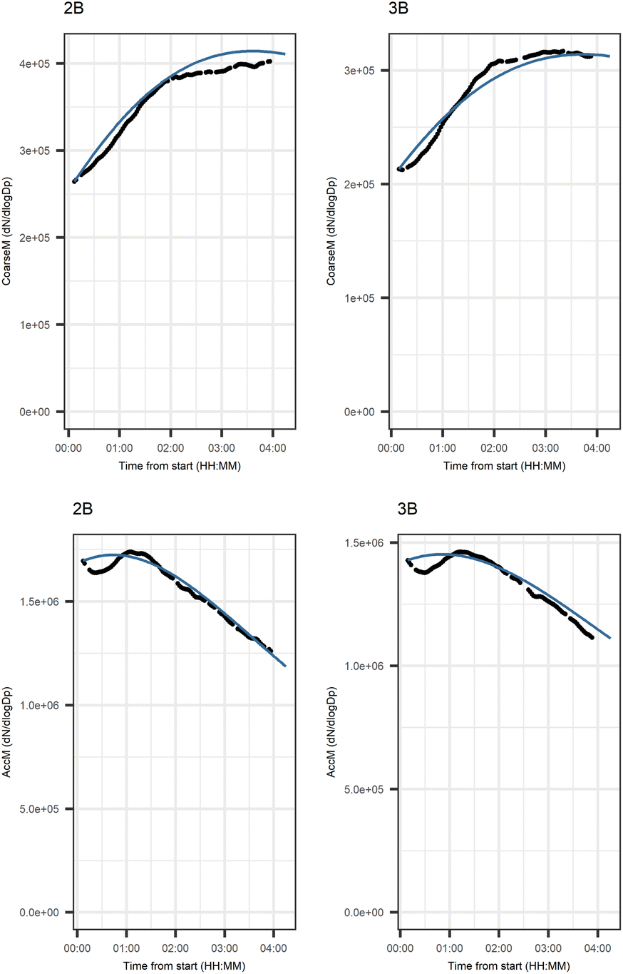Fig. 7 Evolution of the number concentration of coarse (CoarseM, >300 nm) and accumulation mode (AccM, 100–300 nm) particles in dark aging experiments. Black points represent the filtered version of variables and the blue line shows the modeled evolution. For photochemical aging experiments, the difference between the measured and modeled evolution is slightly larger than for dark aging experiments. The largest differences between measured and modeled evolutions were in variables NO and NO₂ on both experiments.

Fig. 6 shows the subgraph of the dependences for particle-size variables. Most of the coefficients are as expected: variables affecting themselves have negative coefficients, thus possibly relating to the coagulation of particles of the same size and hence decreasing the number concentration of the size class. In addition, there are usually negative coefficient for reactions of a variable with a larger size mode, e.g. NuclM × CoarM → NuclM possibly due to coagulation of nucleation mode particles with coarse mode particles. Positive coefficients are mostly related to reactions with smaller sized particles, possibly due to the coagulation of particles resulting in larger particles (e.g. AitM × CoarM → CoarM and AccM × CoarM → CoarM). However, there are some dependencies that do not follow the expectations listed above. As seen in Fig. 7, the modeled evolution is in agreement with the measured one in both experiments. Fig. 8 shows the graph for SOA variables in photochemical aging experiments. For SOA3, which has the most significant increase during the experiments, reactions of O₃ with PTR1 and PTR1 (primary VOCs) and OH reacting with SOA3 are the most important sources. Formation by OH is suggested in Tiitta et al. (2016).¹³ SOA1 is also related to OH and O₃ during photochemical aging, whereas SOA2 is mostly related to reactions with gas-phase products of PTR2 (nitrate/peroxy radicals). Edges O₃ → SOA1 and PTR2 → SOA2 are in line with Tiitta et al. (2016),¹³ whereas OH → SOA1 is not suggested there. Fig. 9 shows the evolution of PTR3 and SOA3. All coefficients for the photochemical aging model and figures for other variables not shown here can be found in the ESI file (ESI S4, Table S9 and Fig. S5–S7).†

Fig. 8 Secondary organic aerosol (SOA)-related part of the causal graph for photochemical aging experiments. SOA factors 1–3 whose evolution is described by other variables are highlighted in green. O₃ is measured from the gas phase, factors PTR1–2 are formed from Proton-Transfer-Reactor Time-of-Flight Mass Spectrometer (PTR-ToF-MS) measurements, the hydroxyl radical (OH) is derived from d9-butanol concentrations, and NO₃ signatured aerosol and SOA1–3 are given by particle-phase measurements with an Aerosol Mass Spectrometer (AMS). PTR factors represent (1) primary VOCs and (2) photochemical aging products and SOA factors represent (1) formation by ozonolysis, (2) formation by nitrate/peroxy radicals, and (3) formation by OH radicals. The color of the arrow represents the sign of the effect, black arrows represent the positive coefficient and red arrows the negative coefficient.

Fig. 9 Evolution of PTR3 and SOA3 factors in photochemical aging experiments. PTR3 is a factor derived from Proton-Transfer-Reactor Time-of-Flight Mass Spectrometer (PTR-ToF-MS) measurements and represents dark aging products; SOA3 is a secondary organic aerosol (SOA) factor derived from Aerosol Mass Spectrometer (AMS) particle-phase measurements and represents compounds that are formed by hydroxyl (OH) radicals. PTR3 represents dark aging products and SOA3 represents formation by OH radicals. Black points represent the filtered version of variable and the blue line shows the modeled evolution.

Fig. 10 shows the subgraph of the dependencies for particle-size variables in photochemical aging experiments. As also seen in dark aging experiments (Fig. 6), most of the estimated coefficients follow the same expectations as listed in a paragraph discussing particle-size variables during dark aging experiments. However, there are also some coefficients that do not conform to expectations. As in the dark aging experiments, there are some positive coefficients between a single variable and a smaller size class (here CoarM → NuclM, CoarM → AccM, and AitM → NuclM) that should be negative due to coagulation. Some interactions between smaller size classes should not physically have a large effect on larger size class number concentration, e.g. NuclM × AitM → CoarM. In addition, in photochemical experiments, the evolution of larger particles is well captured by the model (Fig. 11).

Fig. 10 Particle-size related part of the causal graph for photochemical aging experiments. Particle-size related variables (nucleation mode (NuclM, <25 nm), Aitken mode (AitM, 25–100 nm), accumulation mode (AccM, 100–300 nm), and coarse mode (CoarseM, >300 nm)) are highlighted in green; yellow squares represent interaction variables. All variables are measured using a Scanning Mobility Particle Sizer (SMPS). The color of the arrow represents the sign of the effect; black arrows represent positive coefficient and red arrows the negative coefficient.

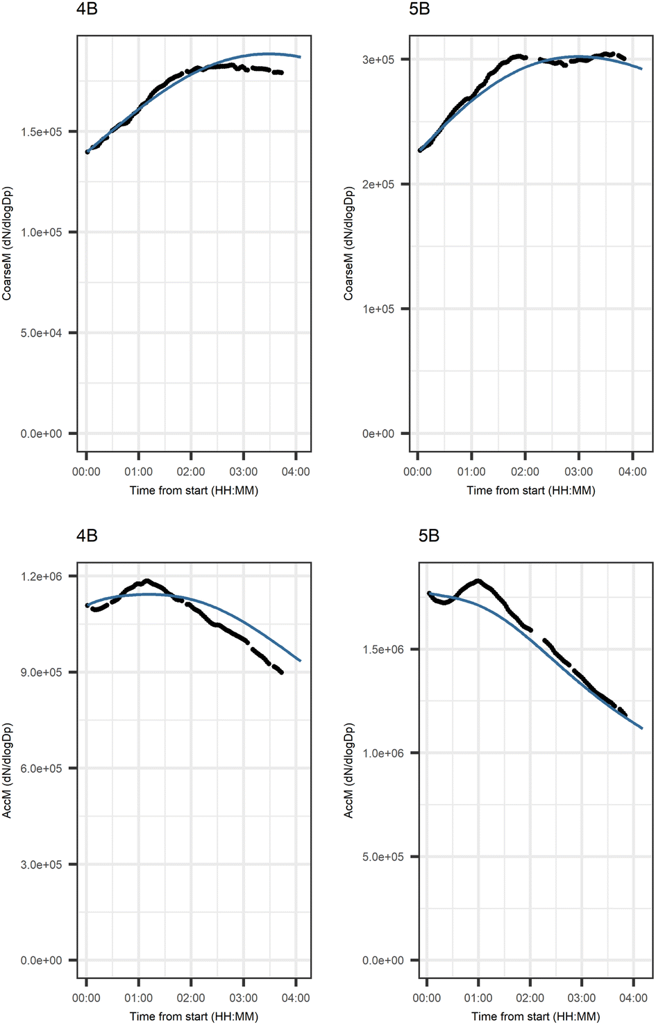Fig. 11 Evolution of the number concentration of coarse (CoarseM, >300 nm) and accumulation mode (AccM, 100–300 nm) particles in photochemical aging experiments. Black points represent the filtered version of the variable and the blue line shows the modeled evolution.

Simulated data mimicking the combustion emissions was used to validate model performance. The aim was to test how the method (causal discovery algorithm + interaction variables + LASSO, see Section 2.2.1) would perform in a situation in which we know the system, in terms of both causal connections between the variables and how the system has evolved during the observation time.

Detailed results from the simulation studies are presented in ESI S3.† In general, we found that most of the dependencies that the algorithm found were correct, or the predictor variables that were suggested to cause a change in the variable Δ(x) had a high correlation with the correct cause. We also found that correct prior information could increase the fraction of exactly correct edges.

We also tested whether it was necessary to use a filtering method for “measured” (simulated + the error mimicking measurement uncertainty) time series before applying a causal discovery algorithm. We found that the filtering method we used for time series reduced the error in the fit when the uncertainty related to the variable was high (Fig. S1†). Also, filtering improved the accuracy of the suggested causal structure if the observed noise in measurements was relatively high.

4 Summary and conclusions

In this study, we showed that a statistical model created for aging of small-scale wood combustion data was able to describe the complex evolution of combustion emissions. Dependencies between the observed time series were studied using a causal discovery algorithm, which provides information on the measured data in two levels of detail. It offers a method to detect the dependencies between variables in measured data and find potential causes for the observed dependencies in the data set. The model was first fitted on simulated data in order to test the accuracy of the fit, the prediction ability of the model, and how the dependency structure is formed for data with known properties. Following that test, the model was fitted on a small-scale wood combustion data set to examine how it performs with real observations. Predictive accuracy of the model can be considered a reasonable measure for many possible applications, where an explicit causal understanding of the system is not needed. Model creation is described step-by-step in Section 2.2 and the solving of the model is based on differential equations (for which the relevant coefficients can be found in Tables S7 and S8†).

As atmospheric measurement data contain large uncertainties, and our measurements of combustion emissions and their aging are no exception, we studied how these uncertainties affect our model by using simulated data sets (see ESI S2, Tables S4 and S5†). Based on the simulations, we filtered the initial time series before applying the model and could reduce the error related to the measurement process, thus making the model and the obtained structure more accurate (see ESI S2 and Fig. S1†). We recommend considering the errors in similar future studies by filtering the data.

With carefully planned chamber experiments in a state-of-the-art facility, we were able to study the dependencies between all measured variables and differentiating correct predictors to explain the variables of interest from variables just covarying with them. This was achieved by controlling the number of compounds such that only a limited number of the possible explaining variables were able to affect the variable of interest. It was then possible to measure whether the supposed interaction between compounds/variables was present or not. It is evident that the modeling of the complete structure and correct causal paths of the evolution of combustion emissions require more initial knowledge about the dependencies between the different gaseous and particulate matter. Additionally, increasing the number of experiments in the model validation would likely lead to a better result, as some of the dependencies detected in some experiments can be neglected in other experiments if those are not causal.

For wood combustion emission experiments, the modeled evolution successfully mimicked the evolution measured in the chamber. Some varying practices in the experiments, such as the ignition type and the resulting changes in combustion efficiency, can affect the composition of the PTR-MS and AMS factors. This might result in varying coefficients in different experiments. Taking this into account, the model described the evolution in the experiments well. Recently, there have been multiple studies applying various dimension reduction techniques on oxidation chamber data sets illustrating that the selection of the technique can have a large impact on the interpretation of the results.^62,83–85 For this type of study (aging of the emission by oxidation), an ideal factorization would include the oxidation products from the same generation in one factor. However, more detailed investigation of the most suitable dimension reduction technique is beyond the scope of this work. In future development of the model, however, the choice of dimension reduction technique should be investigated in more detail.

The presented model used temporal evolution of the compounds in (1) factors calculated for particle- and gas-phase mass spectrometer data and (2) forming a structure for dependencies between compound groups and some specific compounds. It must be acknowledged that our model is not based on the explicit details of the chemical formulae of the compounds nor on the number of carbon and oxygen of the species as is, for example, SOM. In the case of complex systems such as wood combustion, which contains hundreds to thousands of different emission species, explicit knowledge is not available. Thus, the data-based model introduced here can provide important information for further studies on the detailed chemistry of the combustion process.

Based on the simulated experiments, the model captures the evolution well. Most of the dependencies between the variables without causal attribution in the simulated model are co-varying with at least some of the dependencies assumed as causal by the researchers. Due to complex chemistry behind the measured data and a great number of compounds and phenomena not measured in our study, the results of the model cannot directly be interpreted as the causal evolution of the combustion emissions in the atmospheric chamber. However, it can still be taken as a good description of the process. In addition, based on the simulations (see ESI, Tables S6 and S7†), the model could process prior information more efficiently, which is a topic for further development of the model.

The model introduced here provides a step towards a more complete understanding of variable interactions in laboratory experiments considering atmospheric aging. With the introduced model, the dependencies between variables can be detected with lower computational cost than the detailed chemistry models would require. The results of the model give new insight on the data itself and give prior information for more detailed chemical analyses. More research and different observational data sets are still needed for more precise quantification of the dependence structure between the studied variables.

Code and data availability

Codes and data related to this manuscript have been published in Zenodo (DOI: http://10.5281/zenodo.7220521).

Author contributions

SM and JK developed the idea of the study. PT, HC, OS, and AL carried out wood combustion experiments. VL, SM and JK developed the model with substance input from HC, PT and OS. VL and SI performed the data analysis. VL prepared the manuscript with contributions from all co-authors.

Conflicts of interest

The authors declare that they have no conflict of interest.

Acknowledgements

This work was supported by the Academy of Finland Centre of Excellence (grant no. 307331), Academy of Finland Flagship funding (grant no. 337550), the Academy of Finland Competitive funding to strengthen university research profiles (PROFI) for the University of Eastern Finland (grant no. 325022) and for the University of Jyväskylä (grant no. 311877) and the Nessling foundation. Data collection for this study has been partly funded by the European Union's 10 Horizon 2020 Research and Innovation Programme through the EUROCHAMP-2020 Infrastructure Activity (grant no. 730997). Funding sources have no involvement in study design, data analysis, or preparation of the manuscript.

References

1. R. L. Cordell, M. Mazet, C. Dechoux, S. M. L. Hama, J. Staelens, J. Hofman, C. Stroobants, E. Roekens, G. P. A. Kos, E. P. Weijers, K. F. A. Frumau, P. Panteliadis, T. Delaunay, K. P. Wyche and P. S. Monks, Evaluation of biomass burning across North West Europe and its impact on air quality, Atmos. Environ., 2016, 141, 276–286.
2. M. Glasius, A. M. K. Hansen, M. Claeys, J. S. Henzing, A. D. Jedynska, A. Kasper-Giebl, M. Kistler, K. Kristensen, J. Martinsson, W. Maenhaut, J. K. Nøjgaard, G. Spindler, K. E. Stenström, E. Swietlicki, S. Szidat, D. Simpson and K. E. Yttri, Composition and sources of carbonaceous aerosols in Northern Europe during winter, Atmos. Environ., 2018, 173, 127–141.
3. R. M. Qadir, J. Schnelle-Kreis, G. Abbaszade, J. M. Arteaga-Salas, J. Diemer and R. Zimmermann, Spatial and temporal variability of source contributions to ambient PM10 during winter in Augsburg, Germany using organic and inorganic tracers, Chemosphere, 2014, 103, 263–273.
4. J. Hovorka, P. Pokorná, P. K. Hopke, K. Křůmal, P. Mikuška and M. Píšová, Wood combustion, a dominant source of winter aerosol in residential district in proximity to a large automobile factory in Central Europe, Atmos. Environ., 2015, 113, 98–107.
5. C. Reche, M. Viana, F. Amato, A. Alastuey, T. Moreno, R. Hillamo, K. Teinilä, K. Saarnio, R. Seco, J. Peñuelas, C. Mohr, A. S. H. Prévôt and X. Querol, Biomass burning contributions to urban aerosols in a coastal Mediterranean City, Sci. Total Environ., 2012, 427–428, 175–190.
6. J. Orasche, T. Seidel, H. Hartmann, J. Schnelle-Kreis, J. C. Chow, H. Ruppert and R. Zimmermann, Comparison of Emissions from Wood Combustion. Part 1: Emission Factors and Characteristics from Different Small-Scale Residential Heating Appliances Considering Particulate Matter and Polycyclic Aromatic Hydrocarbon (PAH)-Related Toxicological Potential of Particle-Bound Organic Species, Energy Fuels, 2012, 26, 6695–6704.
7. J. Tissari, O. Sippula, J. Kouki, K. Vuorio and J. Jokiniemi, Fine Particle and Gas Emissions from the Combustion of Agricultural Fuels Fired in a 20 kW Burner, Energy Fuels, 2008, 22, 2033–2042.
8. A. K. Frey, K. Saarnio, H. Lamberg, F. Mylläri, P. Karjalainen, K. Teinilä, S. Carbone, J. Tissari, V. Niemelä, A. Häyrinen, J. Rautiainen, J. Kytömäki, P. Artaxo, A. Virkkula, L. Pirjola, T. Rönkkö, J. Keskinen, J. Jokiniemi and R. Hillamo, Optical and Chemical Characterization of Aerosols Emitted from Coal, Heavy and Light Fuel Oil, and Small-Scale Wood Combustion, Environ. Sci. Technol., 2014, 48, 827–836.
9. U. Dusek, G. P. Frank, A. Massling, K. Zeromskiene, Y. Iinuma, O. Schmid, G. Helas, T. Hennig, A. Wiedensohler and M. O. Andreae, Water uptake by biomass burning aerosol at sub- and supersaturated conditions: closure studies and implications for the role of organics, Atmos. Chem. Phys., 2011, 11, 9519–9532.
10. A. Kocbach Bølling, J. Pagels, K. Yttri, L. Barregard, G. Sallsten, P. E. Schwarze and C. Boman, Health effects of residential wood smoke particles: the importance of combustion conditions and physicochemical particle properties, Part. Fibre Toxicol., 2009, 6, 29.
11. M. Hallquist, J. C. Wenger, U. Baltensperger, Y. Rudich, D. Simpson, M. Claeys, J. Dommen, N. M. Donahue, C. George, A. H. Goldstein, J. F. Hamilton, H. Herrmann, T. Hoffmann, Y. Iinuma, M. Jang, M. E. Jenkin, J. L. Jimenez, A. Kiendler-Scharr, W. Maenhaut, G. McFiggans, T. F. Mentel, A. Monod, A. S. H. Prévôt, J. H. Seinfeld, J. D. Surratt, R. Szmigielski and J. Wildt, The formation, properties and impact of secondary organic aerosol: current and emerging issues, Atmos. Chem. Phys., 2009, 9, 5155–5236.
12. U. Pöschl, Atmospheric Aerosols: Composition, Transformation, Climate and Health Effects, Angew. Chem., Int. Ed., 2005, 44, 7520–7540.
13. P. Tiitta, A. Leskinen, L. Hao, P. Yli-Pirilä, M. Kortelainen, J. Grigonyte, J. Tissari, H. Lamberg, A. Hartikainen, K. Kuuspalo, A.-M. Kortelainen, A. Virtanen, K. E. J. Lehtinen, M. Komppula, S. Pieber, A. S. H. Prévôt, T. B. Onasch, D. R. Worsnop, H. Czech, R. Zimmermann, J. Jokiniemi and O. Sippula, Transformation of logwood combustion emissions in a smog chamber: formation of secondary organic aerosol and changes in the primary organic aerosol upon daytime and nighttime aging, Atmos. Chem. Phys., 2016, 16, 13251–13269.
14. A. Bertrand, G. Stefenelli, E. A. Bruns, S. M. Pieber, B. Temime-Roussel, J. G. Slowik, A. S. H. Prévôt, H. Wortham, I. El Haddad and N. Marchand, Primary emissions and secondary aerosol production potential from woodstoves for residential heating: influence of the stove technology and combustion efficiency, Atmos. Environ., 2017, 169, 65–79.
15. E. A. Bruns, M. Krapf, J. Orasche, Y. Huang, R. Zimmermann, L. Drinovec, G. Močnik, I. El-Haddad, J. G. Slowik, J. Dommen, U. Baltensperger and A. S. H. Prévôt, Characterization of primary and secondary wood combustion products generated under different burner loads, Atmos. Chem. Phys., 2015, 15, 2825–2841.
16. J. K. Kodros, D. K. Papanastasiou, M. Paglione, M. Masiol, S. Squizzato, K. Florou, K. Skyllakou, C. Kaltsonoudis, A. Nenes and S. N. Pandis, Rapid dark aging of biomass burning as an overlooked source of oxidized organic aerosol, Proc. Natl. Acad. Sci. U. S. A., 2021, 117, 33028–33033.
17. E. Z. Nordin, O. Uski, R. Nyström, P. Jalava, A. C. Eriksson, J. Genberg, P. Roldin, C. Bergvall, R. Westerholm, J. Jokiniemi, J. H. Pagels, C. Boman and M.-R. Hirvonen, Influence of ozone initiated processing on the toxicity of aerosol particles from small scale wood combustion, Atmos. Environ., 2015, 102, 282–289.
18. L. Künzi, P. Mertes, S. Schneider, N. Jeannet, C. Menzi, J. Dommen, U. Baltensperger, A. S. H. Prévôt, M. Salathe, M. Kalberer and M. Geiser, Responses of lung cells to realistic exposure of primary and aged carbonaceous aerosols, Atmos. Environ., 2013, 68, 143–150.
19. J. Martinsson, A. C. Eriksson, I. E. Nielsen, V. B. Malmborg, E. Ahlberg, C. Andersen, R. Lindgren, R. Nyström, E. Z. Nordin, W. H. Brune, B. Svenningsson, E. Swietlicki, C. Boman and J. H. Pagels, Impacts of Combustion Conditions and Photochemical Processing on the Light Absorption of Biomass Combustion Aerosol, Environ. Sci. Technol., 2015, 49, 14663–14671.
20. N. K. Kumar, J. C. Corbin, E. A. Bruns, D. Massabó, J. G. Slowik, L. Drinovec, G. Močnik, P. Prati, A. Vlachou, U. Baltensperger, M. Gysel, I. El-Haddad and A. S. H. Prévôt, Production of particulate brown carbon during atmospheric aging of residential wood-burning emissions, Atmos. Chem. Phys., 2018, 18, 17843–17861.
21. M. L. Hinks, J. Montoya-Aguilera, L. Ellison, P. Lin, A. Laskin, J. Laskin, M. Shiraiwa, D. Dabdub and S. A. Nizkorodov, Effect of relative humidity on the composition of secondary organic aerosol from the oxidation of toluene, Atmos. Chem. Phys., 2018, 18, 1643–1652.
22. Y. Li, U. Pöschl and M. Shiraiwa, Molecular corridors and parameterizations of volatility in the chemical evolution of organic aerosols, Atmos. Chem. Phys., 2016, 16, 3327–3344.
23. S. M. Platt, I. El Haddad, A. A. Zardini, M. Clairotte, C. Astorga, R. Wolf, J. G. Slowik, B. Temime-Roussel, N. Marchand, I. Ježek, L. Drinovec, G. Močnik, O. Möhler, R. Richter, P. Barmet, F. Bianchi, U. Baltensperger and A. S. H. Prévôt, Secondary organic aerosol formation from gasoline vehicle emissions in a new mobile environmental reaction chamber, Atmos. Chem. Phys., 2013, 13, 9141–9158.
24. A. T. Lambe, P. S. Chhabra, T. B. Onasch, W. H. Brune, J. F. Hunter, J. H. Kroll, M. J. Cummings, J. F. Brogan, Y. Parmar, D. R. Worsnop, C. E. Kolb and P. Davidovits, Effect of oxidant concentration, exposure time, and seed particles on secondary organic aerosol chemical composition and yield, Atmos. Chem. Phys., 2015, 15, 3063–3075.
25. I. J. Keyte, R. M. Harrison and G. Lammel, Chemical reactivity and long-range transport potential of polycyclic aromatic hydrocarbons – a review, Chem. Soc. Rev., 2013, 42, 9333.
26. R. Atkinson, Atmospheric chemistry of VOCs and NO(x), Atmos. Environ., 2000, 34, 2063–2101.
27. V. Vakkari, V.-M. Kerminen, J. P. Beukes, P. Tiitta, P. G. van Zyl, M. Josipovic, A. D. Venter, K. Jaars, D. R. Worsnop, M. Kulmala and L. Laakso, Rapid changes in biomass burning aerosols by atmospheric oxidation, Geophys. Res. Lett., 2014, 41, 2644–2651.
28. A. Kiendler-Scharr, A. A. Mensah, E. Friese, D. Topping, E. Nemitz, A. S. H. Prevot, M. Äijälä, J. Allan, F. Canonaco, M. Canagaratna, S. Carbone, M. Crippa, M. Dall Osto, D. A. Day, P. De Carlo, C. F. Di Marco, H. Elbern, A. Eriksson, E. Freney, L. Hao, H. Herrmann, L. Hildebrandt, R. Hillamo, J. L. Jimenez, A. Laaksonen, G. McFiggans, C. Mohr, C. O'Dowd, R. Otjes, J. Ovadnevaite, S. N. Pandis, L. Poulain, P. Schlag, K. Sellegri, E. Swietlicki, P. Tiitta, A. Vermeulen, A. Wahner, D. Worsnop and H.-C. Wu, Ubiquity of organic nitrates from nighttime chemistry in the European submicron aerosol, Geophys. Res. Lett., 2016, 43, 7735–7744.
29. G. Isaacman-Vanwertz, P. Massoli, R. O'Brien, C. Lim, J. P. Franklin, J. A. Moss, J. F. Hunter, J. B. Nowak, M. R. Canagaratna, P. K. Misztal, C. Arata, J. R. Roscioli, S. T. Herndon, T. B. Onasch, A. T. Lambe, J. T. Jayne, L. Su, D. A. Knopf, A. H. Goldstein, D. R. Worsnop and J. H. Kroll, Chemical evolution of atmospheric organic carbon over multiple generations of oxidation, Nat. Chem., 2018, 10, 462–468.
30. A. Hartikainen, P. Yli-Pirilä, P. Tiitta, A. Leskinen, M. Kortelainen, J. Orasche, J. Schnelle-Kreis, K. E. J. Lehtinen, R. Zimmermann, J. Jokiniemi and O. Sippula, Volatile Organic Compounds from Logwood Combustion: Emissions and Transformation under Dark and Photochemical Aging Conditions in a Smog Chamber, Environ. Sci. Technol., 2018, 52, 4979–4988.
31. A. Hartikainen, P. Tiitta, M. Ihalainen, P. Yli-Pirilä, J. Orasche, H. Czech, M. Kortelainen, H. Lamberg, H. Suhonen, H. Koponen, L. Hao, R. Zimmermann, J. Jokiniemi, J. Tissari and O. Sippula, Photochemical transformation of residential wood combustion emissions: dependence of organic aerosol composition on OH exposure, Atmos. Chem. Phys., 2020, 20, 6357–6378.
32. D. S. Tkacik, E. S. Robinson, A. Ahern, R. Saleh, C. Stockwell, P. Veres, I. J. Simpson, S. Meinardi, D. R. Blake, R. J. Yokelson, A. A. Presto, R. C. Sullivan, N. M. Donahue and A. L. Robinson, A dual-chamber method for quantifying the effects of atmospheric perturbations on secondary organic aerosol formation from biomass burning emissions, J. Geophys. Res. Atmos., 2017, 122, 6043–6058.
33. N. M. Donahue, A. L. Robinson, C. O. Stanier and S. N. Pandis, Coupled partitioning, dilution, and chemical aging of semivolatile organics, Environ. Sci. Technol., 2006, 40, 2635–2643.
34. N. M. Donahue, S. A. Epstein, S. N. Pandis and A. L. Robinson, A two-dimensional volatility basis set: 1. organic-aerosol mixing thermodynamics, Atmos. Chem. Phys., 2011, 11, 3303–3318.
35. G. Ciarelli, I. El Haddad, E. Bruns, S. Aksoyoglu, O. Möhler, U. Baltensperger and A. S. H. Prévôt, Constraining a hybrid volatility basis-set model for aging of wood-burning emissions using smog chamber experiments: a box-model study based on the VBS scheme of the CAMx model (v5.40), Geosci. Model Dev., 2017, 10, 2303–2320.
36. E. A. Bruns, I. El Haddad, J. G. Slowik, D. Kilic, F. Klein, U. Baltensperger and A. S. H. Prévôt, Identification of significant precursor gases of secondary organic aerosols from residential wood combustion, Sci. Rep., 2016, 6, 1–9.
37. A. L. Robinson, N. M. Donahue, M. K. Shrivastava, E. A. Weitkamp, A. M. Sage, A. P. Grieshop, T. E. Lane, J. R. Pierce and S. N. Pandis, Rethinking Organic Aerosols: Semivolatile Emissions and Photochemical Aging, Science, 2007, 315, 1259–1262.
38. B. Zhao, S. Wang, N. M. Donahue, W. Chuang, L. H. Ruiz, N. L. Ng, Y. Wang and J. Hao, Evaluation of one-dimensional and two-dimensional volatility basis sets in simulating the aging of secondary organic aerosol with smog-chamber experiments, Environ. Sci. Technol., 2015, 49, 2245–2254.
39. S. H. Jathar, T. D. Gordona, C. J. Hennigan, H. O. T. Pye, G. Pouliot, P. J. Adams, N. M. Donahue and A. L. Robinson, Unspeciated organic emissions from combustion sources and their influence on the secondary organic aerosol budget in the United States, Proc. Natl. Acad. Sci. U. S. A., 2014, 111, 10473–10478.
40. S. H. Jathar, N. M. Donahue, P. J. Adams and A. L. Robinson, Testing secondary organic aerosol models using smog chamber data for complex precursor mixtures: influence of precursor volatility and molecular structure, Atmos. Chem. Phys., 2014, 14, 5771–5780.
41. G. Stefenelli, J. Jiang, A. Bertrand, E. A. Bruns, S. M. Pieber, U. Baltensperger, N. Marchand, S. Aksoyoglu, A. S. H. Prévôt, J. G. Slowik and I. El Haddad, Secondary organic aerosol formation from smoldering and flaming combustion of biomass: a box model parametrization based on volatility basis set, Atmos. Chem. Phys., 2019, 19, 11461–11484.
42. G. Ciarelli, S. Aksoyoglu, I. El Haddad, E. A. Bruns, M. Crippa, L. Poulain, M. Äijälä, S. Carbone, E. Freney, C. O'Dowd, U. Baltensperger and A. S. H. Prévôt, Modelling winter organic aerosol at the European scale with CAMx: evaluation and source apportionment with a VBS parameterization based on novel wood burning smog chamber experiments, Atmos. Chem. Phys., 2017, 17, 7653–7669.
43. G. Ciarelli, S. Aksoyoglu, M. Crippa, J. L. Jimenez, E. Nemitz, K. Sellegri, M. Äijälä, S. Carbone, C. Mohr, C. O'dowd, L. Poulain, U. Baltensperger and A. S. H. Prévôt, Evaluation of European air quality modelled by CAMx including the volatility basis set scheme, Atmos. Chem. Phys., 2016, 16, 10313–10332.
44. S. M. Saunders, M. E. Jenkin, R. G. Derwent and M. J. Pilling, Protocol for the development of the Master Chemical Mechanism, MCM v3 (Part A): tropospheric degradation of non-aromatic volatile organic compounds, Atmos. Chem. Phys., 2003, 3, 161–180.
45. M. E. Jenkin, S. M. Saunders and M. J. Pilling, The tropospheric degradation of volatile organic compounds: a protocol for mechanism development, Atmos. Environ., 1997, 31, 81–104.
46. B. Aumont, S. Szopa and S. Madronich, Modelling the evolution of organic carbon during its gas-phase tropospheric oxidation: development of an explicit model based on a self generating approach, Atmos. Chem. Phys., 2005, 5, 2497–2517.
47. M. M. Coggon, C. Y. Lim, A. R. Koss, K. Sekimoto, B. Yuan, J. B. Gilman, D. H. Hagan, V. Selimovic, K. J. Zarzana, S. S. Brown, J. M. Roberts, M. Müller, R. Yokelson, A. Wisthaler, J. E. Krechmer, J. L. Jimenez, C. Cappa, J. H. Kroll, J. de Gouw and C. Warneke, OH chemistry of non-methane organic gases (NMOGs) emitted from laboratory and ambient biomass burning smoke: evaluating the influence of furans and oxygenated aromatics on ozone and secondary NMOG formation, Atmos. Chem. Phys., 2019, 19, 14875–14899.
48. C. D. Cappa and K. R. Wilson, Multi-generation gas-phase oxidation, equilibrium partitioning, and the formation and evolution of secondary organic aerosol, Atmos. Chem. Phys., 2012, 12, 9505–9528.
49. A. Akherati, Y. He, M. M. Coggon, A. R. Koss, A. L. Hodshire, K. Sekimoto, C. Warneke, J. De Gouw, L. Yee, J. H. Seinfeld, T. B. Onasch, S. C. Herndon, W. B. Knighton, C. D. Cappa, M. J. Kleeman, C. Y. Lim, J. H. Kroll, J. R. Pierce and S. H. Jathar, Oxygenated Aromatic Compounds are Important Precursors of Secondary Organic Aerosol in Biomass-Burning Emissions, Environ. Sci. Technol., 2020, 54, 8568–8579.
50. J. Pearl, Causality: Models, Reasoning and Inference, Cambridge University Press, 2009.
51. C. Krich, J. Runge, D. G. Miralles, M. Migliavacca, O. Perez-Priego, T. El-Madany, A. Carrara and M. D. Mahecha, Estimating causal networks in biosphere-atmosphere interaction with the PCMCI approach, Biogeosciences, 2020, 17, 1033–1061.
52. J. Runge, P. Nowack, M. Kretschmer, S. Flaxman and D. Sejdinovic, Detecting and quantifying causal associations in large nonlinear time series datasets, Sci. Adv., 2019, 5 DOI:10.1126/sciadv.aau4996.
53. J. Runge, V. Petoukhov, J. F. Donges, J. Hlinka, N. Jajcay, M. Vejmelka, D. Hartman, N. Marwan, M. Paluš and J. Kurths, Identifying causal gateways and mediators in complex spatio-temporal systems, Nat. Commun., 2015, 6, 8502.
54. S. M. Samarasinghe, Y. Deng and I. Ebert-Uphoff, J. Atmos. Sci., 2020, 77, 925–941.
55. I. Ebert-Uphoff and Y. Deng, Causal discovery in the geosciences—using synthetic data to learn how to interpret results, Comput. Geosci., 2017, 99, 50–60.
56. A. Leskinen, P. Yli-Pirilä, K. Kuuspalo, O. Sippula, P. Jalava, M.-R. Hirvonen, J. Jokiniemi, A. Virtanen, M. Komppula and K. E. J. Lehtinen, Characterization and testing of a new environmental chamber, Atmos. Meas. Tech., 2015, 8, 2267–2278.
57. A. A. Reda, H. Czech, J. Schnelle-Kreis, O. Sippula, J. Orasche, B. Weggler, G. Abbaszade, J. M. Arteaga-Salas, M. Kortelainen, J. Tissari, J. Jokiniemi, T. Streibel and R. Zimmermann, Analysis of Gas-Phase Carbonyl Compounds in Emissions from Modern Wood Combustion Appliances: Influence of Wood Type and Combustion Appliance, Energy Fuels, 2015, 29, 3897–3907.
58. H. Czech, O. Sippula, M. Kortelainen, J. Tissari, C. Radischat, J. Passig, T. Streibel, J. Jokiniemi and R. Zimmermann, On-line analysis of organic emissions from residential wood combustion with single-photon ionisation time-of-flight mass spectrometry (SPI-TOFMS), Fuel, 2016, 177, 334–342.
59. S. S. Brown and J. Stutz, Nighttime radical observations and chemistry, Chem. Soc. Rev., 2012, 41, 6405.
60. T. B. Onasch, A. Trimborn, E. C. Fortner, J. T. Jayne, G. L. Kok, L. R. Williams, P. Davidovits and D. R. Worsnop, Soot Particle Aerosol Mass Spectrometer: Development, Validation, and Initial Application, Aerosol Sci. Technol., 2012, 46, 804–817.
61. P. Barmet, J. Dommen, P. F. DeCarlo, T. Tritscher, A. P. Praplan, S. M. Platt, A. S. H. Prévôt, N. M. Donahue and U. Baltensperger, OH clock determination by proton transfer reaction mass spectrometry at an environmental chamber, Atmos. Meas. Tech., 2012, 5, 647–656.
62. S. Isokääntä, E. Kari, A. Buchholz, L. Hao, S. Schobesberger, A. Virtanen and S. Mikkonen, Comparison of dimension reduction techniques in the analysis of mass spectrometry data, Atmos. Meas. Tech., 2020, 13, 2995–3022.
63. W. Revelle, psych: Procedures for Psychological, Psychometric, and Personality Research, Evanston, Illinois, 2018.
64. R Core Team, R: A Language and Environment for Statistical Computing, Vienna, Austria, 2019.
65. A. L. Comrey, A First Course in Factor Analysis, Academic Press, 1973.
66. A. G. Yong and S. Pearce, A Beginner's Guide to Factor Analysis: Focusing on Exploratory Factor Analysis, Tutor. Quant. Methods Psychol., 2013, 9, 79–94.
67. M. R. Canagaratna, J. T. Jayne, J. L. Jimenez, J. D. Allan, M. R. Alfarra, Q. Zhang, T. B. Onasch, F. Drewnick, H. Coe, A. Middlebrook, A. Delia, L. R. Williams, A. M. Trimborn, M. J. Northway, P. F. DeCarlo, C. E. Kolb, P. Davidovits and D. R. Worsnop, Chemical and microphysical characterization of ambient aerosols with the aerodyne aerosol mass spectrometer, Mass Spectrom. Rev., 2007, 26, 185–222.
68. J. de Gouw and C. Warneke, Measurements of volatile organic compounds in the earth's atmosphere using proton-transfer-reaction mass spectrometry, Mass Spectrom. Rev., 2007, 26, 223–257.
69. L. E. Hatch, R. J. Yokelson, C. E. Stockwell, P. R. Veres, I. J. Simpson, D. R. Blake, J. J. Orlando and K. C. Barsanti, Multi-instrument comparison and compilation of non-methane organic gas emissions from biomass burning and implications for smoke-derived secondary organic aerosol precursors, Atmos. Chem. Phys., 2017, 17, 1471–1489.
70. B. Yuan, A. R. Koss, C. Warneke, M. Coggon, K. Sekimoto and J. A. de Gouw, Proton-Transfer-Reaction Mass Spectrometry: Applications in Atmospheric Sciences, Chem. Rev., 2017, 117, 13187–13229.
71. P. Paatero, Least squares formulation of robust non-negative factor analysis, Chemom. Intell. Lab. Syst., 1997, 37, 23–35.
72. I. M. Ulbrich, M. R. Canagaratna, Q. Zhang, D. R. Worsnop and J. L. Jimenez, Interpretation of organic components from Positive Matrix Factorization of aerosol mass spectrometric data, Atmos. Chem. Phys., 2009, 9, 2891–2918.
73. J. H. Kroll, N. M. Donahue, J. L. Jimenez, S. H. Kessler, M. R. Canagaratna, K. R. Wilson, K. E. Altieri, L. R. Mazzoleni, A. S. Wozniak, H. Bluhm, E. R. Mysak, J. D. Smith, C. E. Kolb and D. R. Worsnop, Carbon oxidation state as a metric for describing the chemistry of atmospheric organic aerosol, Nat. Chem., 2011, 3, 133–139.
74. W. S. Cleveland, Robust Locally Weighted Regression and Smoothing Scatterplots, J. Am. Stat. Assoc., 1979, 74, 829.
75. C. Wongchokprasitti, rcausal: R-Causal Library, 2019.
76. R. Tibshirani, Regression Shrinkage and Selection via the Lasso, J. R. Stat. Soc., B: Stat. Methodol., 1996, 58, 267–288.
77. K. Soetaert, T. Petzoldt and R. W. Setzer, Solving Differential Equations in R: Package deSolve, J. Stat. Softw., 2010, 33, 1–25.
78. P. Spirtes, C. N. Glymour and R. Scheines, Causation, Prediction, and Search, MIT Press, 2000.
79. X. Shen, S. Ma, P. Vemuri, G. Simon, M. W. Weiner, P. Aisen, R. Petersen, C. R. Jack, A. J. Saykin, W. Jagust, J. Q. Trojanowki, A. W. Toga, L. Beckett, R. C. Green, J. Morris, L. M. Shaw, Z. Khachaturian, G. Sorensen, M. Carrillo, L. Kuller, M. Raichle, S. Paul, P. Davies, H. Fillit, F. Hefti, D. Holtzman, M. M. Mesulam, W. Potter, P. Snyder, A. Schwartz, T. Montine, R. G. Thomas, M. Donohue, S. Walter, D. Gessert, T. Sather, G. Jiminez, A. B. Balasubramanian, J. Mason, I. Sim, D. Harvey, M. Bernstein, N. Fox, P. Thompson, N. Schuff, C. DeCArli, B. Borowski, J. Gunter, M. Senjem, D. Jones, K. Kantarci, C. Ward, R. A. Koeppe, N. Foster, E. M. Reiman, K. Chen, C. Mathis, S. Landau, N. J. Cairns, E. Franklin, L. Taylor-Reinwald, V. Lee, M. Korecka, M. Figurski, K. Crawford, S. Neu, T. M. Foroud, S. Potkin, K. Faber, S. Kim, K. Nho, L. Thal, N. Buckholtz, M. Albert, R. Frank, J. Hsiao, J. Kaye, J. Quinn, L. Silbert, B. Lind, R. Carter, S. Dolen, L. S. Schneider, S. Pawluczyk, M. Beccera, L. Teodoro, B. M. Spann, J. Brewer, H. Vanderswag, A. Fleisher, J. L. Heidebrink, J. L. Lord, S. S. Mason, C. S. Albers, D. Knopman, K. Johnson, R. S. Doody, J. Villanueva-Meyer, V. Pavlik, V. Shibley, M. Chowdhury, S. Rountree, M. Dang, Y. Stern, L. S. Honig, K. L. Bell, B. Ances, M. Carroll, M. L. Creech, M. A. Mintun, S. Schneider, A. Oliver, D. Marson, D. Geldmacher, M. N. Love, R. Griffith, D. Clark, J. Brockington, E. Roberson, H. Grossman, E. Mitsis, R. C. Shah, L. deToledo-Morrell, R. Duara, M. T. Greig-Custo, W. Barker, C. Onyike, D. D'Agostino, S. Kielb, M. Sadowski, M. O. Sheikh, A. Ulysse, M. Gaikwad, P. M. Doraiswamy, J. R. Petrella, S. Borges-Neto, T. Z. Wong, E. Coleman, S. E. Arnold, J. H. Karlawish, D. A. Wolk, C. M. Clark, C. D. Smith, G. Jicha, P. Hardy, P. Sinha, E. Oates, G. Conrad, O. L. Lopez, M. A. Oakley, D. M. Simpson, A. P. Porsteinsson, B. S. Goldstein, K. Martin, K. M. Makino, M. S. Ismail, C. Brand, A. Preda, D. Nguyen, K. Womack, D. Mathews, M. Quiceno, A. I. Levey, J. J. Lah, J. S. Cellar, J. M. Burns, R. H. Swerdlow, W. M. Brooks, L. Apostolova, K. Tingus, E. Woo, D. H. S. Silverman, P. H. Lu, G. Bartzokis, N. R. Graff-Radford, F. Parfitt, K. Poki-Walker, M. R. Farlow, A. M. Hake, B. R. Matthews, J. R. Brosch, S. Herring, C. H. van Dyck, R. E. Carson, M. G. MacAvoy, P. Varma, H. Chertkow, H. Bergman, C. Hosein, S. Black, B. Stefanovic, C. Caldwell, G.-Y. R. Hsiung, B. Mudge, V. Sossi, H. Feldman, M. Assaly, E. Finger, S. Pasternack, I. Rachisky, J. Rogers, D. Trost, A. Kertesz, C. Bernick, D. Munic, E. Rogalski, K. Lipowski, S. Weintraub, B. Bonakdarpour, D. Kerwin, C.-K. Wu, N. Johnson, C. Sadowsky, T. Villena, R. S. Turner, K. Johnson, B. Reynolds, R. A. Sperling, K. A. Johnson, G. Marshall, J. Yesavage, J. L. Taylor, B. Lane, A. Rosen, J. Tinklenberg, M. N. Sabbagh, C. M. Belden, S. A. Jacobson, S. A. Sirrel, N. Kowall, R. Killiany, A. E. Budson, A. Norbash, P. L. Johnson, T. O. Obisesan, S. Wolday, J. Allard, A. Lerner, P. Ogrocki, C. Tatsuoka, P. Fatica, E. Fletcher, P. Maillard, J. Olichney, O. Carmichael, S. Kittur, M. Borrie, T.-Y. Lee, R. Bartha, S. Johnson, S. Asthana, C. M. Carlsson, P. Tariot, A. Burke, A. M. Milliken, N. Trncic, S. Reeder, V. Bates, H. Capote, M. Rainka, D. W. Scharre, M. Kataki, B. Kelly, E. A. Zimmerman, D. Celmins, A. D. Brown, G. D. Pearlson, K. Blank, K. Anderson, L. A. Flashman, M. Seltzer, M. L. Hynes, R. B. Santulli, K. M. Sink, L. Gordineer, J. D. Williamson, P. Garg, F. Watkins, B. R. Ott, G. Tremont, L. A. Daiello, S. Salloway, P. Malloy, S. Correia, H. J. Rosen, B. L. Miller, D. Perry, J. Mintzer, K. Spicer, D. Bachman, N. Pomara, R. Hernando, A. Sarrael, S. K. Schultz, K. E. Smith, H. Koleva and The Alzheimer's Disease Neuroimaging Initiative, Challenges and Opportunities with Causal Discovery Algorithms: Application to Alzheimer's Pathophysiology, Sci. Rep., 2020, 10, 2975.
80. J. H. Seinfeld and S. N. Pandis, Atmospheric Chemistry and Physics, Wiley, 2016.
81. P. Wang, Gibbs Sampler for Bayesian Lasso, https://cs.gmu.edu/%7Epwang7/gibbsBLasso.html, accessed, 13 December 2019.
82. T. Park and G. Casella, The Bayesian Lasso, J. Am. Stat. Assoc., 2008, 103, 681–686.
83. A. Buchholz, A. Ylisirniö, W. Huang, C. Mohr, M. Canagaratna, D. R. Worsnop, S. Schobesberger and A. Virtanen, Deconvolution of FIGAERO–CIMS thermal desorption profiles using positive matrix factorisation to identify chemical and physical processes during particle evaporation, Atmos. Chem. Phys., 2020, 20, 7693–7716.
84. A. R. Koss, M. R. Canagaratna, A. Zaytsev, J. E. Krechmer, M. Breitenlechner, K. J. Nihill, C. Y. Lim, J. C. Rowe, J. R. Roscioli, F. N. Keutsch and J. H. Kroll, Dimensionality-reduction techniques for complex mass spectrometric datasets: application to laboratory atmospheric organic oxidation experiments, Atmos. Chem. Phys., 2020, 20, 1021–1041.
85. B. Rosati, R. Teiwes, K. Kristensen, R. Bossi, H. Skov, M. Glasius, H. B. Pedersen and M. Bilde, Factor analysis of chemical ionization experiments: numerical simulations and an experimental case study of the ozonolysis of α-pinene using a PTR-ToF-MS, Atmos. Environ., 2019, 199, 15–31.
86. A. T. Ahern, E. S. Robinson, D. S. Tkacik, R. Saleh, L. E. Hatch, K. C. Barsanti, C. E. Stockwell, R. J. Yokelson, A. A. Presto, A. L. Robinson, R. C. Sullivan and N. M. Donahue, Production of Secondary Organic Aerosol During Aging of Biomass Burning Smoke From Fresh Fuels and Its Relationship to VOC Precursors, J. Geophys. Res. Atmos., 2019, 124(6), 3583–3606.

---

Footnotes

† Electronic supplementary information (ESI) available. See DOI: https://doi.org/10.1039/d2ea00048b

‡ Now at: Finnish Meteorol. Inst., Atmospher. Res. Ctr Eastern Finland, Kuopio FI-70211, Finland.

§ Now at: Cooperation group “Comprehensive Molecular Analytics (CMA)”, Helmholtz Zentrum München, 81379 München, Germany.

---