
 Open Access Article
 This Open Access Article is licensed under a Creative Commons Attribution-Non Commercial 3.0 Unported Licence
Elucidating the impacts of COVID-19 lockdown on air quality and ozone chemical characteristics in India†
Behrooz
Roozitalab
 *ab,
Gregory R.
Carmichael
*ab,
Sarath K.
Guttikunda
c and
Maryam
Abdi-Oskouei
d
*ab,
Gregory R.
Carmichael
*ab,
Sarath K.
Guttikunda
c and
Maryam
Abdi-Oskouei
d
aChemical and Biochemical Engineering, University of Iowa, Iowa City, IA, USA
bCenter for Global and Regional Environmental Research, University of Iowa, Iowa City, IA, USA. E-mail: Behrooz-roozitalab@uiowa.edu; gcarmich@engineering.uiowa.edu
cUrban Emissions, New Delhi, India
dUniversity Corporation for Atmospheric Research (UCAR), Boulder, CO, USA
First published on 25th July 2022
Abstract
India implemented a stay-at-home order (i.e. lockdown) on 24 March 2020 to decrease the spread of novel COVID-19, which reduced air pollutant emissions in different sectors. The Weather Research and Forecasting model with Chemistry (WRF-Chem) was used to better understand the processes controlling the changes in PM2.5 and ozone in northern India during the lockdown period, including (1) the contributions of inter-annual variability in meteorology and emissions (dust, biogenic, and biomass burning) and lockdown emissions to changes in PM2.5 and ozone in northern India and (2) to analyze changes in ozone production regimes due to the lockdown. We found that both meteorology and lockdown emissions contributed to daytime PM2.5 (−12% and −12%, respectively) and ozone (−8% and −5%, respectively) reduction averaged in April 2020 in the Indo-Gangetic Plain, and in smaller magnitudes in northern India. However, the ozone concentration response to reductions in its precursors (i.e. NO2 and VOCs) due to the lockdown emissions was not constant over the domain. While the ozone concentration decreased in most parts of the domain, it occasionally increased in major cities like Delhi and in regions with many power plants. We utilized the reaction rate information in WRF-Chem to study the ozone chemistry. We found carbon monoxide, formaldehyde, isoprene, acetaldehyde, and ethylene as the major VOCs that contribute to the ozone formation in India. We used the ratio of radical termination from radical–radical interactions to radical–NOx interactions, and its corresponding formaldehyde to NO2 ratio (FNR) to find the ozone chemical regimes. We showed that the FNR transition range in a region depends on whether it is an urban, rural, or power plant region. Using the FNR information, we found that most parts of India are within the NOx-limited regime. We also found that large emission reduction during the lockdown period shifted the chemical regimes toward NOx-limited although it did not necessarily change the chemical regime in many VOC-limited regions. The results of this study highlight the fact that reducing the exposure to both PM2.5 and ozone requires air pollution management strategies that consider both NOx and VOC emission reductions, and that take into account regional characteristics.
Environmental significanceThe COVID-19 lockdown in India led to large reductions in air pollutant emissions. Here, we investigate the contributions of inter-annual variability in meteorology and COVID-19 lockdown emissions to changes in PM2.5 and ozone in northern India and analyze changes in ozone production regimes due to the lockdown. We demonstrate that both meteorology and lockdown emissions contributed to air quality changes in April 2020 (i.e. the lockdown period) compared to April 2019. Furthermore, we show that large emission reduction during the COVID-19 lockdown shifted the chemical regimes toward NOx-limited although it did not necessarily change the chemical regime in many VOC-limited regimes. These findings improve our understanding on why the pollutants responded the way they did, which is needed in order to use the lessons learned from the COVID-19 lockdown to inform future air quality management strategies. |
Introduction
While the COVID-19 virus is a global disaster in terms of its health and economy damage, it provides a unique opportunity to enhance our understanding of earth system sciences.1 As many countries initiated stay-at-home orders (hereafter called lockdown) in early 2020 to control the spread of the virus, anthropogenic air pollutant emissions started to decline in different sectors.2 While many past studies have explored the impacts of future stringent emission control “scenarios” on air quality,3 the worldwide lockdowns provide a real-world scenario accompanied by actual observations on how the air quality responded. As a result, many studies have been undertaken to document the changes in air quality during the lockdown periods. Comprehensive reviews can be found in Gkatzelis, et al.4 and Sokhi, et al.5 However, further work is needed to better understand why the pollutants responded the way they did. This understanding is needed in order to use the lessons learned from the COVID-19 lockdown to inform future air quality management strategies.In this study, we look into the processes controlling the changes in pollution levels in northern India. Air pollution is a major concern in India due to its large health and environmental impacts.6,7 While even extreme air pollution events are not unusual in India,8 clean air due to the lockdown was unusual and attracted people's and media's attention.9 In India, the lockdown officially started on 24 March 2020 and continued in four phases until the end of May 2020. While residential and power sector emissions did not show large changes, large emission reductions were reported in other sectors such as transportation.10 This reduction in emissions resulted in different changes in air quality over India. The relatively short lifetime of NO2 makes it a suitable tracer of local NOx emissions11 and satellite retrieved tropospheric column NO2 concentrations showed large reductions over Delhi and other urban regions, due to the lower activities in the transportation sector (Fig. 1). However, the demand for electricity showed small changes during the lockdown period; NO2 concentrations did not change very much over the thermal power plant region.12 Other studies using TROPOspheric Monitoring Instrument (TROPOMI) and Ozone Monitoring Instrument (OMI) satellites and ground measurement data showed similar changes.13,14
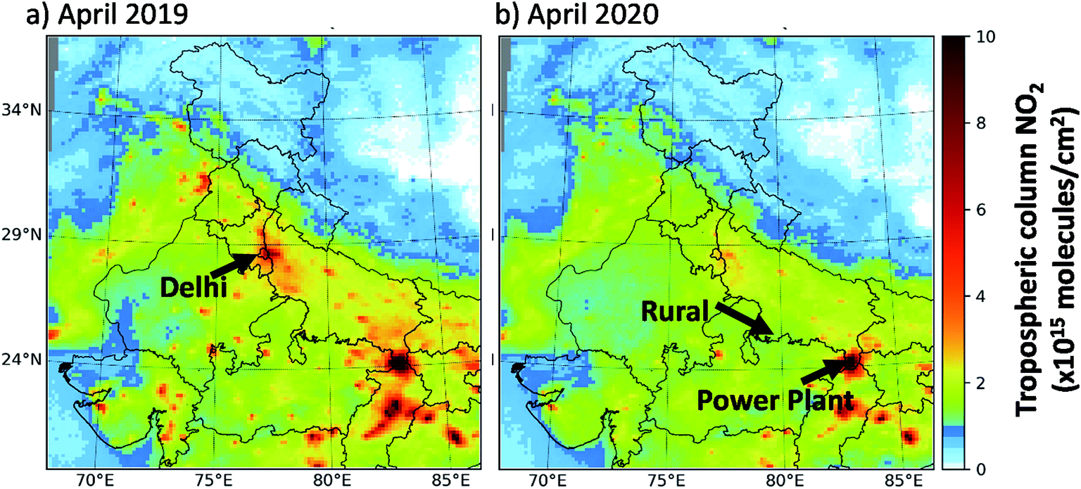 | ||
| Fig. 1 Tropospheric column NO2 concentrations over the WRF-Chem modeling domain averaged for April (a) 2019 and (b) 2020 retrieved from TROPOMI on board the Copernicus Sentinel-5 Precursor satellite. The three regions used for process analysis have been marked and also shown in Fig. S1.† The quality assurance of more than 0.5 was used. | ||
Many studies have used measurement data to quantify the changes in air pollutant concentrations in Indian regions during different phases of the lockdown period.15–20 They found significant reductions in PM2.5 and NO2 concentrations when compared to the pre-lockdown period or previous years. A more limited number of modeling studies have also investigated the lockdown effects in India by performing simulations with emissions perturbed to mimic the lockdown period. Zhang, et al.21 used the WRF-CMAQ model to study the pre-lockdown-to-lockdown air quality changes in India, between 21 February and 24 April 2020, by decreasing the emissions in industrial (82%), transportation (85%), and energy (26%) sectors during the lockdown period. Dumka, et al.22 used the WRF-CHIMERE model and simulated significantly lower PM2.5 and NO2 concentrations over India during the lockdown period (between 25 March and 17 May 2020) compared with the pre-lockdown period by completely excluding traffic and industrial sectors from the emission inventory. Several studies have used estimates of the changes in emissions during the lockdown, based on activity data2 or top-down emission estimates, to study changes in pollution levels using global models.23,24 These regional and global studies show consistent findings over India, with large decreases in NO2 (40–58%) and generally smaller decreases in PM2.5 (26–55%). However, the responses of ozone were more complicated and varied by study. At some locations and times ozone decreased during the lockdown, but at other locations and times ozone increased during the lockdown.17,25
The different responses of ozone to changes in its precursors are due to its complicated chemistry, where production rates are dependent on the emissions of both NOx and volatile organic compounds (VOCs), with responses determined by which of these is limiting the production. For example, Chen, et al.26 studied the sensitivity of ozone formation to its precursors in Delhi and VOCs were the limiting factor in ozone production; as a result very large reductions in NOx emissions (more than 65–80%) were needed to reduce the ozone concentrations.
Ideally, one would like to directly relate the observed changes in pollutants to changes in emissions due to the lockdown. These observation-based sensitivities would be very helpful in informing air quality management strategies (e.g., a transport-focused strategy that reduced NOx emissions by 20% is expected to reduce PM2.5 by x and ozone by y). However, the attribution of the changes in ambient pollution levels to emission changes during the lockdown is not straightforward. It is complicated by the fact that emissions during the lockdown period are highly uncertain. It is also compounded by the fact that some fraction of the changes are not due to emissions, but due to other factors such as changes in meteorology from year to year.27 For example, Goldberg, et al.28 showed that meteorological conditions alone decreased tropospheric column NO2 concentrations by a median of 21.6% in the United States in 2020 compared with 2019. Gkatzelis, et al.4 found only about one-third of all the global studies on the effects of COVID-19 accounted for impacts of changing meteorology.
The objective of this study is to better understand the processes controlling the changes in PM2.5 and ozone in northern India, with the goals of (1) quantifying the contributions of inter-annual variability in meteorology and emissions (dust, biogenic, and biomass burning) and COVID-19 lockdown emissions to changes in PM2.5 and ozone in northern India and (2) analyzing changes in ozone production regimes due to the lockdown. Ozone levels are high in India and there is growing awareness of the need to consider both PM2.5 and ozone in air quality management strategies. To achieve these goals, we used the regional Weather Research and Forecasting Model with Chemistry (WRF-Chem) version 4 to simulate the air quality during March and April in 2019 and 2020. We also utilized the Integrated Reaction Rate (IRR) capability in this version to understand how ozone formed in different regions (i.e. urban, non-urban, and a thermal power plant region) in northern India and how it changed during the lockdown period. To account for emission changes during the COVID-19 lockdown period, we used the adjustment factors proposed by Doumbia, et al.2
The paper is organized as follows. First, we provide a description of the WRF-Chem model and adjustment factors used to account for the lockdown period emissions, and evaluate the modeling results against ground measurement data in 2019 and 2020. Then, we study the effects of meteorology and lockdown emissions on air quality using different modeling experiments. Moreover, we use the IRR and study the ozone chemistry in different regions in India. Finally, we discuss the sensitivity of the results to the accuracy of the emission inventories and provide a summary of the findings.
Methods
WRF-Chem modeling
WRF-Chem model version 4.0 was used in this study in order to utilize its new IRR capability.29,30 We used a single domain, centered over Delhi, which covered the Indo-Gangetic Plain (IGP) and central India with a 15 km × 15 km resolution and 39 vertical layers (Fig. 1; the location of the IGP is shown in Fig. S12†). The Model for Ozone and Related chemical Tracers, version 4 (MOZART-4) introduced by Emmons, et al.31 with updates on isoprene oxidations32 was selected as the gas phase chemistry mechanism (more information on the evolution of the MOZART mechanism can be found in Emmons, et al.33). For aerosol representation, the four-bin Model for Simulations Aerosol Interactions and Chemistry (MOSAIC-4bin) introduced by Zaveri, et al.34 with updates for Secondary Organic Aerosol (SOA) formation35 was selected. In general, this SOA mechanism is an empirical parameterization scheme that emits two CO-scaled VOC precursor surrogates on behalf of anthropogenic and biomass burning sources (i.e. VOCA and VOCBB). These VOC precursor surrogates react with the hydroxyl (OH) radical and form a non-volatile product that completely condenses to the aerosol phase.35 The SOA formation from biogenic sources follows the two-product oxidation model. Although the mechanism of this scheme is not as robust as the volatility basis set,36 it is a common scheme for regional air quality models as it does not require detailed information on the VOC emissions and is computationally not expensive (e.g. ref. 30 and 37). Furthermore, the SOA formation from glyoxal is also included in this mechanism.32 The current IRR module in the model only works with MOZART gas phase chemistry coupled with this simple SOA parameterization.Initial and boundary conditions (IC/BC) for meteorological fields were provided by National Center for Atmospheric Prediction Global Forecasting System Final Analysis (NCEP GFS-FNL) data (https://rda.ucar.edu/datasets/ds083.2/, last access: 20 December 2020). For Chemical IC/BC, we used the Whole Atmosphere Community Climate Model (WACCM) outputs.38 We reinitialized the model every 30 hours and updated meteorological IC/BC and chemical boundary conditions but used the chemical initial condition from the previous cycle. The re-initialization for every cycle started during nighttime at 1800 UTC (2330 Local Time (LT)) and the first 6 hours were discarded as spin up following Abdi-Oskouei, et al.39 The simulation period included March and April in 2019 and 2020, while we primarily focus on April results. The details of other configuration options can be found in Roozitalab, et al.8
Emissions
There are several global anthropogenic emission inventories publicly available including the Hemispheric Transport of Air Pollution emission inventory (HTAP v2.2), Copernicus Atmosphere Monitoring Service global emission inventory version 4.2 (CAMS v4.2), and Community Emissions Data System (CEDS). However, they are different in terms of the emission factors, base year of the fuel use and activity data, horizontal resolution of the data, etc. resulting in different emission magnitudes.40–42 We used the modified CEDS (CEDS_M) emission inventory as our base anthropogenic emission inventory.43 McDuffie, et al.43 updated the emissions for India based on a gridded national emission inventory developed by Venkataraman, et al.44 Nevertheless, we used HTAP v2.2 data for the air sector, as CEDS_M does not have data for this sector. They mapped the total VOC emissions to 25 individual VOC species based on the data from the RETRO project.43 The mapping between these VOCs and WRF-Chem emission species is provided in Table S1† (personal communications with Louisa Emmons, NCAR). A comparison between the emissions in CEDS_M and two other global inventories (i.e. HTAP v2.2 and CAMS v4.2) over the studied domain can be found in the ESI.†To consider emission reductions due to the lockdown in 2020, we used the adjustment factors (AFs) provided by Doumbia, et al.2 Doumbia, et al.2 estimated the global gridded AFs based on the change of activity data for each sector with respect to a five-week period starting January 2020. Fig. 2 shows the daily change of emissions for (a) India, and three pre-defined box regions, (b) Urban, (c) Power, and (d) Rural. It shows a small fluctuation in emissions until 24 March (as adjusting factors are with regard to January), with a dramatic change afterwards due to initiation of the lockdown. The lockdown had a large impact on NOx emission with about 30% reduction averaged over India. The emissions of SO2 also showed large reductions (∼40%) with smaller reductions (∼10%) for Non Methane Volatile Organic Carbons (NMVOCs; hereafter NMVOCs refer to VOCs except methane and CO and VOCs refer to their inclusion) and CO. While black carbon decreased over India, Organic Carbon (OC) increased during the lockdown due to increased fuel consumption for the residential sector.45 The total changes in emission in each region depend on both the AFs and the amount of emissions from each sector in that region (Tables S2 and S3†). The Urban and Power showed emission reductions for all the species. However, VOCs, BC, and OC increased over Rural. This increase is due to the emissions from the residential sector, which is the dominant one in rural areas over northern India. Fig. 2(e and f) also show the maps of averaged emission reductions in April 2020 for NMVOC and NOx. While these results are qualitatively consistent with results in Gaubert, et al.,23 there are some quantitative differences, primarily due to different base emission inventories (CAMS emission inventory) and regions (all of India) they considered. For example in our domain, residential and industrial sectors contribute to 49% and 39% of NMVOC emissions, respectively, in the CAMS inventory while their corresponding contributions in the CEDS_M inventory are 60% and 7% (more details can be found in the ESI†). Therefore, the increased activity in the residential sector during the lockdown would show larger impacts when using the CEDS_M inventory.
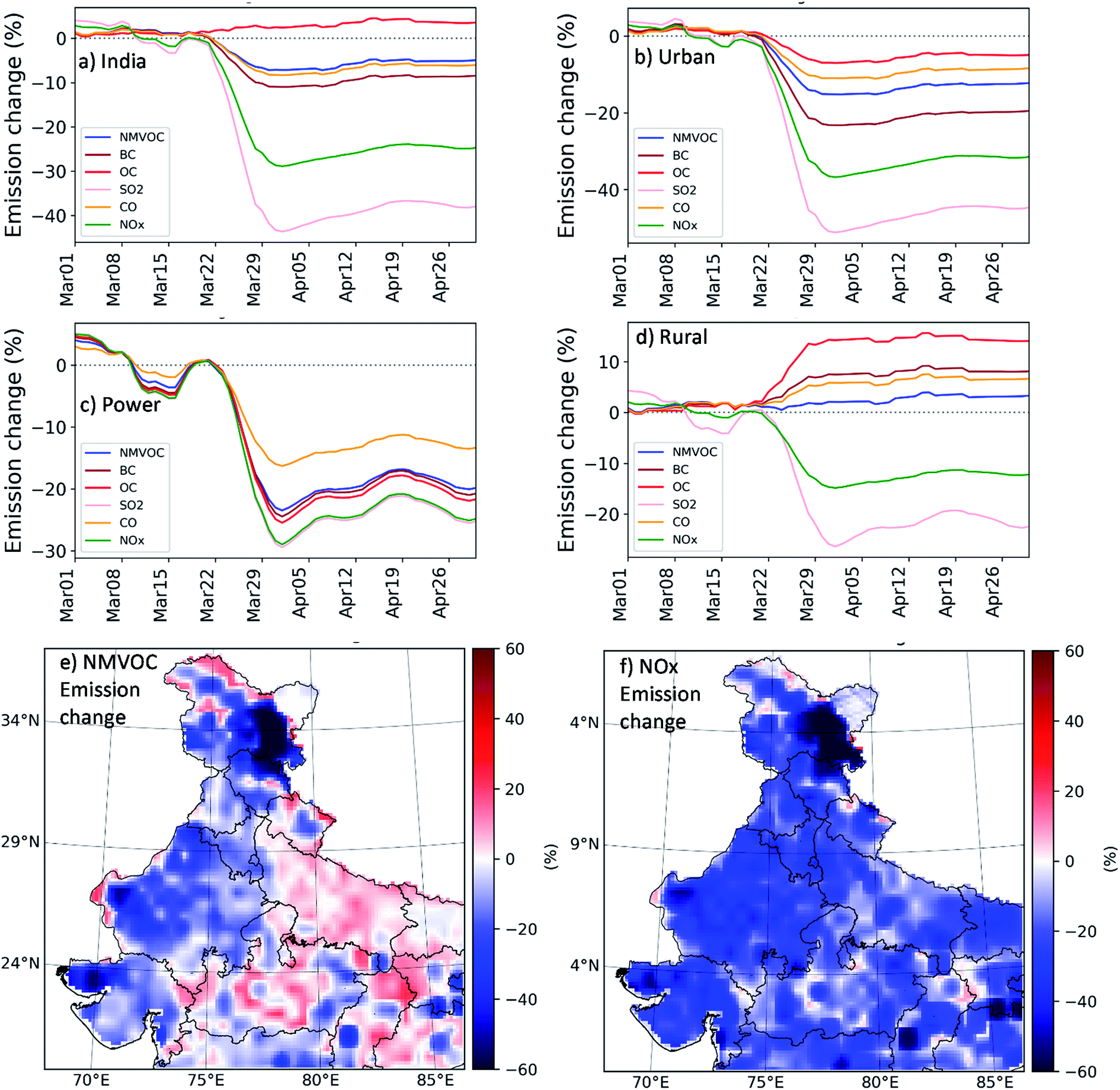 | ||
| Fig. 2 Daily emission change due to AF applied on CEDS_M emissions averaged in (a) India, (b) Urban, (c) Power, and (d) Rural (X-axis shows the days in March and April and the Y-axis range is different for each subplot). Map of emission changes of (e) NMVOC and (f) NOx averaged in April 2020. The location of the box regions can be found in the ESI.† | ||
The Fire Inventory from NCAR, version 2.2 (FINN v2.2) based on MODIS fire detections was used as the biomass burning emission inventory.46 Comparing the fire emissions between 2019 and 2020 during the studied period showed lower total emissions in 2020 (Fig. S2†), with most of the fires over central parts of the domain. However, it also showed that some days in 2020 (e.g. 16 April) had much larger emissions compared with 2019. We also used the online Model of Emissions of Gases and Aerosols from Nature (MEGAN v2.0.4) as the biogenic emission inventory.47 MEGAN emissions changed between the years 2019 and 2020 as they are based on meteorological fields (i.e. temperature). The total amount of biogenic and biomass burning emissions in April 2019 and April 2020 is provided in Table S4.† For dust emissions, we used the online Goddard Global Ozone Chemistry Aerosol Radiation and Transport (GOCART) mechanism.
Simulations
To study the response of air quality to both meteorological and emission forcings, we performed four simulations (Table 1). It should be noted the we considered all emission sources that are directly (i.e. biogenic and wind-blown dust) and indirectly (biomass burning) related to meteorology as meteorological forcings. The reason is that the lockdown anthropogenic emissions' adjustments do not directly affect these sources. In the 2019BAU (BAU: Business As Usual) scenario, all the year-dependent input data including chemical and meteorological IC/BC, and biomass burning emissions were from 2019. As a result, online biogenic and dust emissions also followed the 2019 meteorology. Moreover, we used the CEDS_M emission inventory as BAU anthropogenic emission in 2019BAU. Following the same logic, 2019COVID means 2019 year-dependent input data, while anthropogenic emissions were adjusted based on the multiplication of CEDS_M and AFs for each sector. It should be mentioned that we used the same AFs for both years 2019 and 2020 to account for reduced emission scenarios (i.e. 2019COVID and 2020COVID). Similarly, 2020BAU was based on 2020 year-dependent input data and BAU anthropogenic emission, while 2020COVID used adjusted emissions. These four scenarios provide an opportunity to look at the effects of meteorology, emissions, and their combined effects on air quality over the domain.| Scenario | Meteorology | Anth. emission | Biomass burning emission | Biogenic emission | Dust emission | Initial/boundary condition |
|---|---|---|---|---|---|---|
| 2019BAU | 2019 | CEDS_M | 2019 | 2019 | 2019 | 2019 |
| 2019COVID | 2019 | CEDS_M adjusted with AF | 2019 | 2019 | 2019 | 2019 |
| 2020BAU | 2020 | CEDS_M | 2020 | 2020 | 2020 | 2020 |
| 2020COVID | 2020 | CEDS_M adjusted with AF | 2020 | 2020 | 2020 | 2020 |
Ozone formation analysis
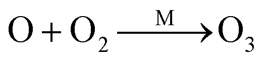
It is important to understand the general processes in the ozone chemistry; we provide a simplified overview of the complex chemistry of ozone in the troposphere. While NOx and VOCs (including CO, and methane (CH4)) are the main precursors of ozone, the OH radical is also a key species in the ozone chemistry. The reason is that OH can oxidize VOCs and produce organic peroxy radicals (RO2) as shown in reaction (1). Then, RO2 can react with NO and produce NO2 without involving ozone (reaction (2): for simplicity, we do not show the pathway towards hydroperoxyl radical (HO2) formation), which can eventually lead to net ozone via reactions (3) and (4). On the other hand, the ozone photolysis is the main source of tropospheric OH. Thus, this loop (reactions (1)–(4)) continues to form ozone during daytime (hv) as far as VOCs and OH are available in the atmosphere (NOx acts more as a catalyst in this loop). Relative to VOCs, CO and CH4 react very slowly with OH. Thus, short-lived VOCs become important as their availability primarily depends on their emissions. However, we should emphasize that it does not necessarily mean that large amounts of VOCs will increase ozone (i.e. radical loss via radicals (LROx)). In terms of OH, it can also react with NO2 and form nitric acid (HNO3), and remove both OH (and other radicals) and NO2 (reaction (5); this is the main reaction of radical loss via NOx termination (LNOx)). In other words, VOC reactivity with OH (VOC + OH) shows a path to ozone formation (reaction (1)), and NO2 reactivity with OH (NO2 + OH) presents an obstacle to ozone formation (reaction (5)). During nighttime, photolysis of NO2 (reaction (3)) does not occur, halting the ozone formation cycle; rather, NO2 reacts with ozone and form gas phase radical nitrate (NO3) through reaction (6). Moreover, available NO consumes ozone and produces NO2 (reaction (7)), accelerating NO3 chemistry, resulting in net ozone destruction. More detailed chemistry of ozone can be found elsewhere (e.g. Pusede and Cohen;48 Seinfeld and Pandis49). We use the reaction rate information from the IRR package in the WRF-Chem model to understand the ozone chemical regime in northern India.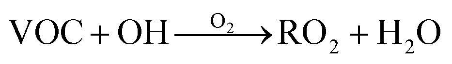 | (1) |
| RO2 + NO → RO + NO2 | (2) |
| NO2 + hν → NO + O | (3) |
 | (4) |
 | (5) |
| NO2 + O3 → NO3 + O2 | (6) |
| NO + O3 → NO2 + O2 | (7) |
To help analyze how the results vary by location we chose three box regions representing an urban, a rural, and a power plant region when analyzing the ozone chemistry based on the population and emission data (Fig. 1). The urban region, with a population of ∼28 million people based on the Gridded Population of the World, Version 4,50 contains the greater Delhi region (hereafter called Urban). The rural area contains a non-urban region with low population (1.4 million) and with very low SO2 emission (Table S3†) in the border of Uttar Pradesh and Madhya Pradesh states (hereafter called Rural), and the power plant region covers a non-urban area with low population (1.3 million) and large SO2 emissions (Table S3†) representing thermal power plants (hereafter called Power). To keep the regions comparable with each other, each region includes a set of 4 × 5 grid cells in the model (∼4500 km2; Fig. S1†). Nevertheless, we consider all the urban, rural, and power plant grid cells in the “FNR and VOC/NOX sensitivities” section for a general conclusion. Hereafter, we also call the Indian regions of the domain as India. The amount of CEDS_M emissions for different species over these defined regions for the month of March and April is shown in the ESI† (Tables S2 and S3). The Urban had the highest emissions for all the species except for NOx and SO2. The NOx and SO2 emissions were higher in Power although the amount of NOx emission was comparable in Urban and Power regions. On the other hand, NMVOC emissions were very low in Power and Rural. Emissions in April were lower than in March for all the regions; however, this difference was very small for Rural as the emissions were originally low.
We also chose two sample days representing pre-lockdown and lockdown conditions to look at the ozone chemistry in defined Urban, Power, and Rural regions. In order to choose these two days, we applied a meteorological filter in Urban to select the days with the most similar meteorology between the years 2019 and 2020. We calculated the daytime averaged 10 meter wind speed and 2 meter temperature for each day in both years and found the day with the lowest overall normalized biases (Fig. S16†). As a result, 13 March and 7 April were selected as the sample pre-lockdown and lockdown days, respectively. Nevertheless, it is important that these days were selected based on the filters in Urban and did not necessarily represent the lowest-meteorological-variability days in Power and Rural (Fig. S16†). As an experiment, we applied the same methodology over India and found two other days with the least variability over the domain. However, it did not mainly affect the following analysis (not shown). We acknowledge that this technique of choosing the days does not consider the effects of previous days and other potential factors like precipitation. It should be mentioned that we consider all the days of April in the “FNR and VOC/NOX sensitivities” section for a general conclusion.
Model evaluation
We evaluated the performance of the model compared with ground measurements and global reanalysis data. Scenarios 2019BAU and 2020COVID should represent the real states of the atmosphere for the years 2019 and 2020, respectively. In the following model evaluation discussion, the model for 2019 refers to 2019BAU and the model for 2020 refers to 2020COVID results in the month of April. For meteorological fields, we compared the model with the Modern-Era Retrospective analysis for Research and Applications, Version 2 (MERRA-2) data.51 Hourly statistics for a location in Delhi (28.6 N, 77.19 E) showed 2 m temperature (T2m) mean error (ME) of 2.9 °C and 3.5 °C in April 2019 and April 2020, respectively, and 10 m wind speed (WS10m) of 1.3 m s−1 and 1.3 m s−1 in April 2019 and April 2020, respectively. The root mean square error (RMSE) for T2m was 3.4 °C and 4.1 °C in April 2019 and April 2020, respectively. The RMSE for WS10m was 1.7 m s−1 and 1.6 m s−1 for April 2019 and April 2020, respectively. These are comparable with Zhang, et al.21 values when modeling the pre-lockdown and lockdown period in India. The model satisfied the wind speed ME goal of 2.0 m s−1, while overestimated the temperature ME goal of 2.0 °C, proposed by Emery, et al.52 The model simulated the daytime (1000–1700 LT) T2m peaks but overestimated nighttime values (Fig. S3†). Fig. 3 shows the averaged hourly T2m over the domain for April 2019 and April 2020 in the model and MERRA-2. The model captured the general spatial pattern of temperature in both April 2019 and April 2020. However, the model was biased low over most parts of India in April 2019. On the other hand, the model was biased high over the IGP and biased low over central India in April 2020. It also shows that the model was biased high over the western parts of the IGP in both April 2019 and April 2020. Comparing WS10m also indicated the ability of the model to capture the spatial pattern, while the model was biased low most of the time in Delhi (Fig. S4†). Overall, the model was capable of simulating the meteorology within the studied periods. The differences in the meteorology, between 2019 and 2020, can affect the air quality by changing the natural emission sources (e.g. dust and biogenic emissions). Furthermore, the dynamics of the atmosphere (e.g. boundary layer height, precipitation, and wind) change how the air pollutants disperse, transport, and deposit in the atmosphere. For example, Fig. S5† shows more precipitation in April 2020 compared with April 2019 in the model, which leads to wet removal of pollutants. The modeled higher precipitation in April 2020 is consistent with the Integrated Multi-satellitE Retrievals for Global precipitation measurement (IMERG) dataset53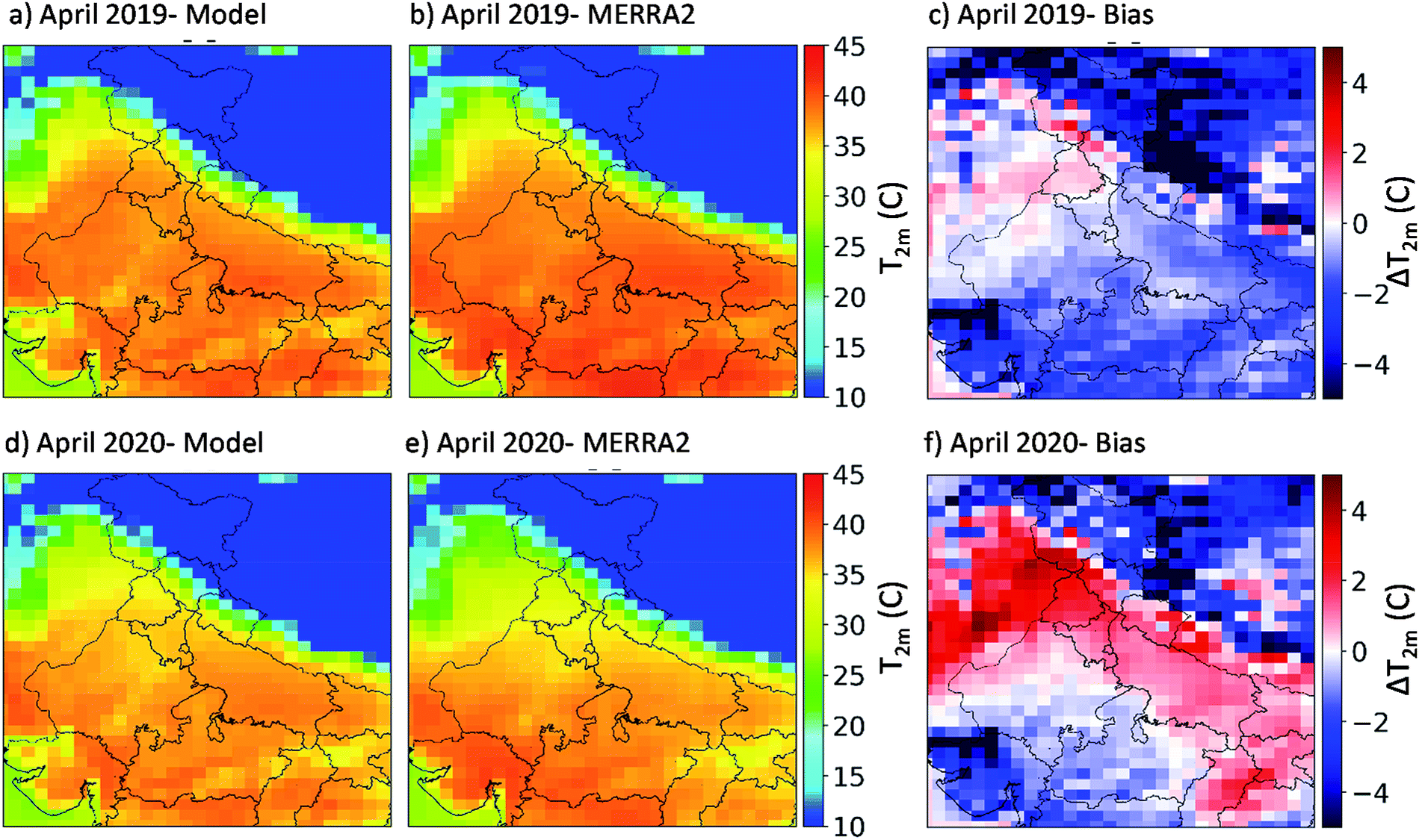 | ||
| Fig. 3 Averaged hourly 2 m temperature in April 2019 (top row) and 2020 (bottom row) in the WRF-Chem model (left column), MERRA-2 (middle column), and their difference (right column). Model results were re-gridded to MERRA-2 resolution. | ||
We used the hourly ground measurement air pollutant concentration data in Delhi collected by the Central Pollution Control Board (CPCB) to evaluate the air quality in the years 2019 and 2020. Other than the original quality control filters applied by the CPCB (https://cpcb.nic.in/quality-assurance-quality-control/, last access: 02/23/2021), we applied four additional filters.20,54 First, we removed the stations with all zero or not-a-number (i.e. NAN) values. Second, we removed the stations with no variation, in which the standard deviation (STD) of the data was less than five percent of its mean. Third and fourth, we removed the outlier values, in which the difference between two consecutive hours was more than 100 units (except for carbon monoxide (CO), for which we used a cut-off of 500 μg m−3) or the difference between each value and the mean value was higher or lower than 3 × STD.
The normalized mean bias (NMB) for daily PM2.5 was −17% and +11% in April 2019 and April 2020, respectively (Table S5†). Although the model performance changes from under-prediction in 2019 to over-prediction in 2020, the daily NMB values for PM2.5 are relatively low and within the benchmark criteria of Emery, et al.55 Similarly, the daily NO2 concentrations were biased low in April 2019 (NMB of −15%) and biased high in April 2020 (NMB of +38%). The predictions were biased high for maximum daily 8 h average (MDA8) ozone mixing ratios with NMB of +18% and +36% in April 2019 and April 2020, respectively. In other words, the model was biased high for ozone in both years. Overall, most of the modeled hourly data points were within the 1:2 lines in both April 2019 and 2020 (Fig. S6†) and the model performance was within the reported values in other studies For example, Kota, et al.56 modeled air quality in India in 2015 and reported NMB of 53% and −33% for ozone and NO2, respectively, in Delhi. Other studies have also reported overestimation of simulated ozone concentrations over Delhi.57–61 We performed an experiment using the HTAP v2.2 emission inventory, which similarly led to biased high ozone mixing ratios (Table S6†). Prediction of air pollutants in India remains a challenge due to large uncertainties in natural (dust) and anthropogenic (including agricultural fires) emissions as many studies have shown.14,62,63 While data assimilation within air quality prediction systems has significantly improved air quality results64 and there are large on-going efforts in developing high-resolution emission inventories for separate sectors or individual cities,65–67 efforts are still needed to integrate all these useful available information in future studies. Another parameter leading to biased high ozone could be the transboundary ozone transport.68 We found that the transported ozone from boundaries could mix with the air in the boundary layer and affect surface concentrations over the domain (more information is provided in the ESI†). In other words, the dynamics of the model and the model capability in correctly capturing the boundary layer height over India could also affect the ozone predictions.8 Furthermore, correct interpolation of global model data into vertical levels of the regional model can also affect the results. Multi-scale models with the capability to simulate regional air quality of a domain in high resolution while resolving other parts of the world in a coarser resolution, all in one framework could remove this interpolation bias.69 In this study, we simply decreased the boundary condition ozone by 50%, which led to ∼20 ppb less surface ozone concentrations. Nevertheless, future studies considering the impact of boundary conditions on ozone over India, evaluating the performance of the model in reproducing the boundary layer, and finding a better adjusting factor for transboundary ozone are needed as it is still biased high.
Fig. 4 shows the measured (black dashed line) and modeled (green line) difference for PM2.5 (panel a), NO2 (panel b), and ozone (panel c) between 2020 and 2019 averaged daytime concentrations in Delhi between 10 March and 30 April Both measured data and the model showed, in general, similar values in 2019 and 2020 between 10 March and around 24 March (before the lockdown) accompanied by a drop afterwards (during the lockdown). However, the day that concentrations dropped is slightly different between the measured data (22 March) and the model (24 March). Yadav, et al.45 also reported that the lockdown was not abrupt and had a transition start. Furthermore, the averaged amount that concentrations dropped during the lockdown period (24 March–30 April) in 2020 compared with 2019 was different between the measured data and the model. Mean reduction for daytime PM2.5 concentrations was 25 μg m−3 in the measured data, while the model showed a smaller drop (9 μg m−3). For daytime NO2, the measured data decreased by 14 μg m−3 (i.e. 48%), while the modeled outputs decreased by 4 μg m−3 (34%). This is lower than 61% that Vadrevu, et al.70 reported based on TROPOMI tropospheric column NO2 concentrations between 25 March and 3 May in 2020 compared with 2019. The difference between the modeled and observed NO2 reduction can be explained in part by the sectoral contribution of the used emission inventory. In particular, the transportation sector is not a major source of NOx in the Urban region (Fig. S28†) within the CEDS_M inventory; the modeled reduction is less significant compared with the results for the HTAP inventory (Fig. S11†). Large uncertainties in NOx emissions from the transportation sector are also reported for other regions.71 Nevertheless, the model was able to capture the overall changes in NO2 columns when compared with TROPOMI data (Fig. S10†). The daytime ozone mixing ratio also dropped during the lockdown in both measured (11 ppb) and modeled (5 ppb) data. However, the 24-hour averaged ozone mixing ratio did not change very much neither in the measured data nor in the model although small fluctuations were observed between years 2019 and 2020 (Fig. S7 and S8†). We will further analyze the ozone response in the process analysis of the ozone chemistry section. Although April 2019 daytime ozone mixing ratios were higher than those of March 2019, we observed lower daytime ozone mixing ratios in April 2020 compared with March 2020, both in the model and measured data (Fig. S9†). This may be seen in contrast with what other studies that reported slightly higher ozone in Delhi during the lockdown compared with the pre-lockdown period.15,18 These differences are primarily due to the methodology and the observed time period. For example, Jain and Sharma15 reported an increase in daily ozone while we report the daytime ozone. On the other hand, Mahato, et al.18 looked at MDA8 ozone during two weeks in the lockdown period compared with two weeks in the pre-lockdown period and reported less than 1% increase. Overall, the model was able to capture the major responses to the lockdown.
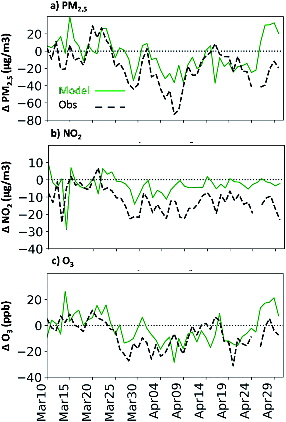 | ||
| Fig. 4 Averaged daytime (1000–1700 LT) PM2.5 (top row), NO2 (middle row), and ozone (bottom row) concentration changes in 2020 and 2019, between 10 March and 30 April, based on the measured data over CPCB stations in Delhi (black dashed line) and modeled data (green solid line) over the Urban region. The observed data were extracted from the ground measurement data in Delhi, while the modeled data were averaged in the Urban box region. | ||
Results
Model responses to meteorology, emission, and combined effects
To compare the air quality during the lockdown period (April 2020) with regard to the previous year, it is important to note that not only emissions but also the meteorology changed. Indeed, meteorology can affect both the transport of the pollution and natural source emissions (i.e. biogenic and biomass burning emissions, Table S4†). Fig. 5 shows the differences in 2 m temperature, biogenic isoprene emission, and biomass burning NOx emission averaged during the daytime over the domain in April 2020 and April 2019. The western IGP had lower temperatures in April 2020 while the eastern IGP and the state of Gujarat experienced warmer days. Because of higher temperatures, the online MEGAN module estimated up to 10% more biogenic isoprene emissions in eastern parts of the IGP in April 2020. On the other hand, it estimated up to 10% lower isoprene emissions in the western IGP in April 2020. Furthermore, biomass burning emissions in the IGP were lower in April 2020 with small fires in the eastern IGP. Overall, the eastern IGP had higher biogenic emissions in April 2020, while biomass burning emissions were lower. In central India, biomass burning emissions were higher in April 2020 compared with April 2019. Due to such changes in meteorology and its related (e.g. biogenic) emissions, the effects of reducing anthropogenic emissions on regional air quality could be different depending on the applied year. Fig. 6 shows the effects of emission reductions due to the lockdown in the years 2019 (the difference between 2019COVID and 2019BAU scenarios) and 2020 (the difference between 2020COVID and 2020BAU scenarios) on averaged daytime PM2.5, NOx, and ozone in the Urban region. While the effect of lockdown emissions on the PM2.5 concentration was relatively large in both years, the averaged effect of the meteorological year was negligible in the Urban region. The effect of emission reductions on changes in the daytime PM2.5 concentration in 2019 was −6 μg m−3 and it was −5.6 μg m−3 in 2020. Similarly, the averaged effect of emission perturbation on changes in the daytime ozone concentration was −1.4 ppb and −1.7 ppb in 2019 and 2020, respectively. For NOx, the emission perturbation effect was similar in both 2019 and 2020 and the effect of meteorology was the least as anthropogenic sources are the main driver of NOx in urban regions. Nevertheless, we found some large differences in day-to-day comparison for these species. For example, lockdown emissions in 2019 and 2020 decreased daytime PM2.5 concentrations in Urban by ∼14 μg m−3 and ∼7 μg m−3, respectively, on 5 April, which corresponds to ∼50% difference due to the year applied. Moreover, the amount of reduction in the NOx mixing ratio on 14 April was different by 50% (4 ppb and 2 ppb in 2019 and 2020, respectively). On the other hand, we also observed contradictory responses on some days. For example, ozone mixing ratios in Urban decreased on 14 April 2019 due to the lockdown emissions, while 2020 data showed an increase.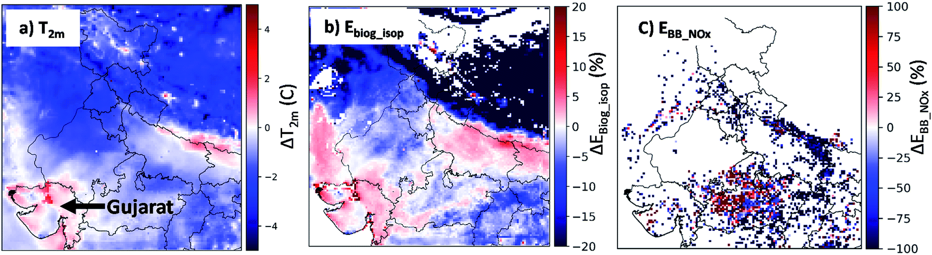 | ||
| Fig. 5 Difference between April 2020 and 2019 in modeled daytime averaged (a) 2 m temperature, (b) biogenic isoprene, and (c) biomass burning NOx emissions over the domain. The changes in EBB_NOx are also true for other biomass burning species such as CO. | ||
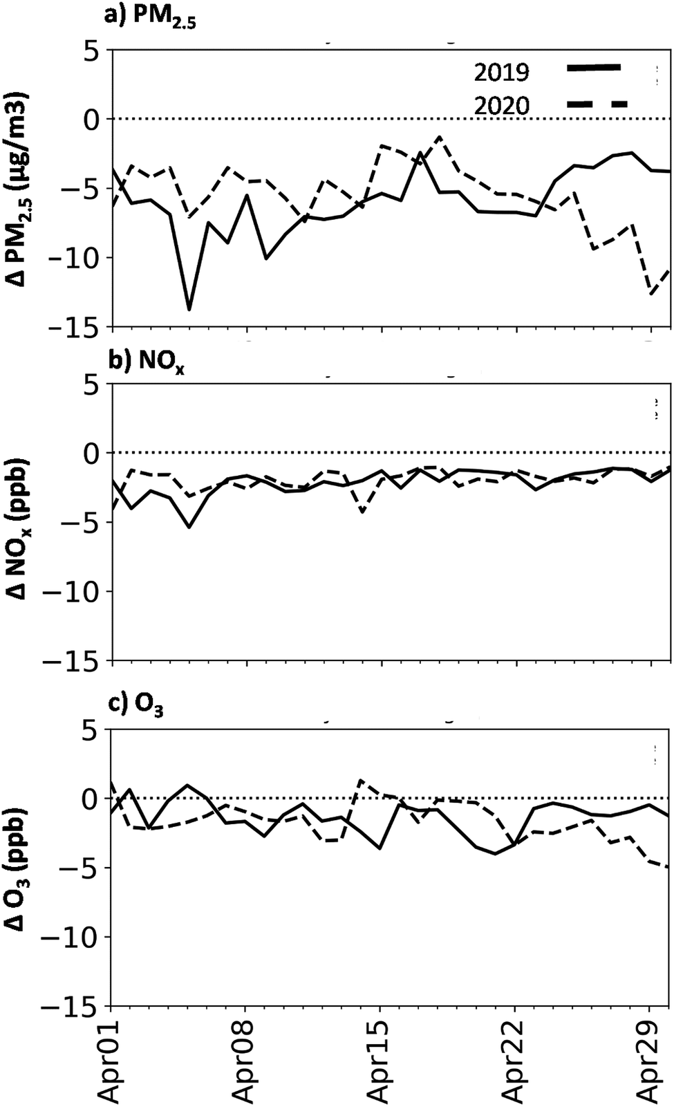 | ||
| Fig. 6 Effect of lockdown emissions on daytime (a) PM2.5, (b) NOx, and (c) ozone concentrations in April 2019 (solid line; difference between 2019COVID and 2019BAU) and 2020 (dashed line; difference between 2020COVID and 2020BAU). | ||
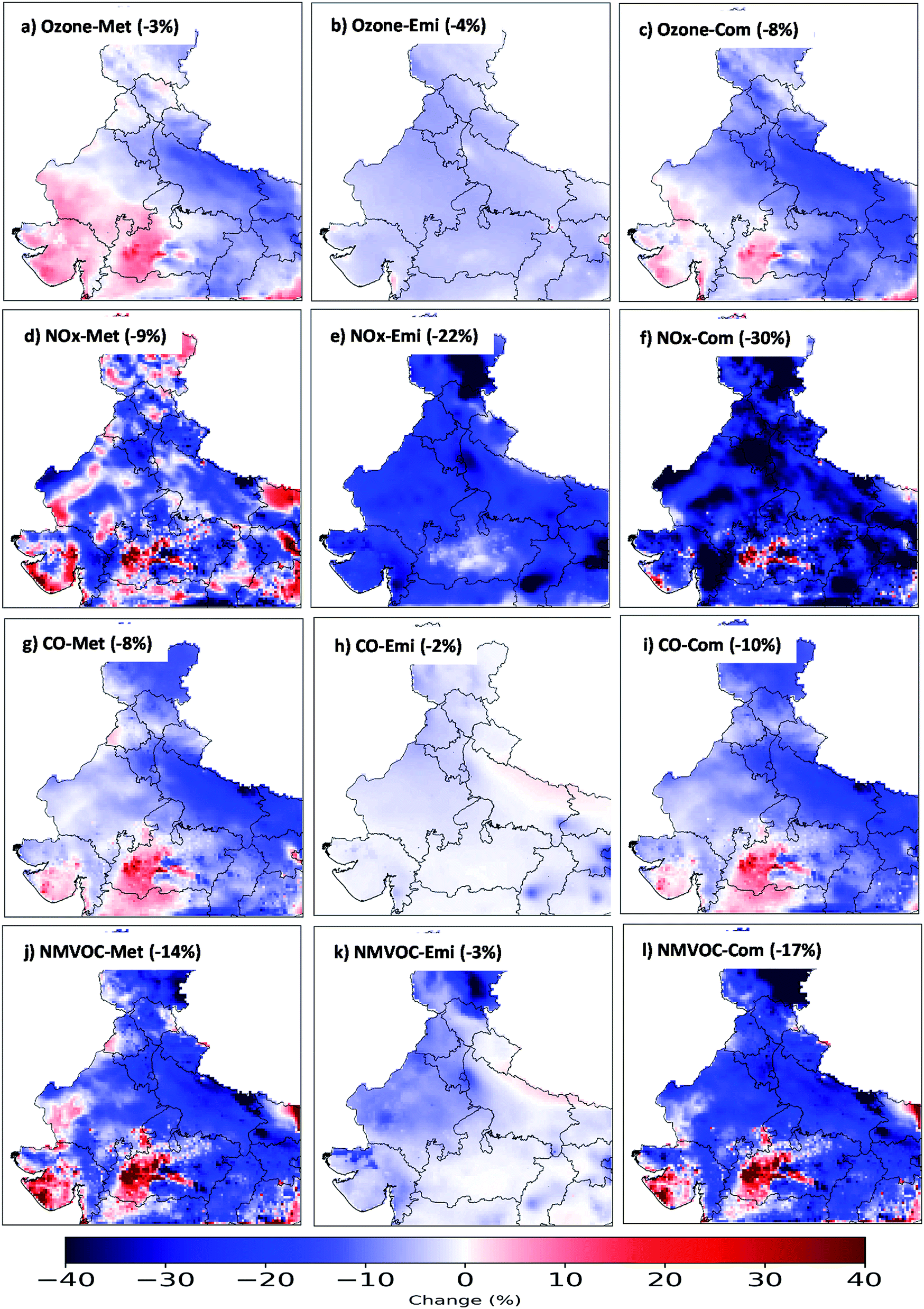
In order to attribute the changes between April 2019 and 2020 over the domain, we looked at three scenarios. The difference between 2020BAU and 2019BAU indicates the effects of meteorology, while the difference between 2020COVID and 2020BAU presents the effects of lockdown emissions. Fig. 7 and 8 show the percentage of point-to-point changes due to meteorology, emissions, and their combined effects (the difference between 2020COVID and 2019BAU) on averaged daytime concentrations in April. Moreover, Table S7† summarizes these changes over India, IGP, and the three predefined representative regions (i.e. Urban, Rural, and Power). In the following analysis, we focus only on India. Similar plots for the IGP region are provided in the ESI† (Fig. S12 and S13).
 | ||
| Fig. 7 Responses of April averaged daytime PM2.5 (first row), PA2.5 (second row), SIA2.5 (third row), and SOA2.5 (fourth row) concentrations to meteorology (left column), emission (middle column), and combined (right column) effects. The numbers in parentheses show the averaged change over the colored region between April 2020 and 2019. | ||
 | ||
| Fig. 8 Responses of April averaged daytime ozone (first row), NOx (second row), CO (third row), and NMVOC (fourth row) concentrations to meteorology (left column), emission (middle column), and combined (right column) effects. The numbers in parentheses show the averaged change over the colored region between April 2020 and 2019. | ||
The averaged daytime PM2.5 concentrations in April in India decreased by only two percent due to the meteorology effects. However, each region in the domain showed different changes (Table S7†). Fig. 7 shows larger PM2.5 concentration reductions over the IGP due to the meteorology effects (Fig. S12† shows 12% for the IGP). The reduction was more intense in some parts of the IGP, e.g. west of Delhi (∼25%). It also shows that PM2.5 concentrations increased over central India by more than 20% over the regions mostly affected by biomass burning emissions. On the other hand, the lockdown emissions decreased PM2.5 concentrations almost everywhere in India (i.e. the IGP and central India) with the average of 9% and the maximum of ∼20% in Delhi. The combined effects show a large reduction in PM2.5 concentrations over the IGP (up to 40%). However, the increase due to the meteorology over central India offsets the decrease due to the lockdown emissions. Overall, the impacts of meteorology and its related emissions (i.e. biogenic, dust, and biomass burning) outweigh impacts of the anthropogenic emissions over most parts of India.
The changes in the PM2.5 composition as primary aerosols (PA2.5; sum of organic carbon, black carbon, and primary inorganics), secondary inorganic aerosols (SIA2.5; sum of nitrate, sulfate, and ammonium), and secondary organic aerosols (SOA2.5) are also shown. Based on the 2019BAU scenario, PA2.5 (48%) were the dominant components of PM2.5 over India in April, with SIA2.5 (39%) and SOA2.5 (13%) including the rest (Fig. S14†). Patel, et al.72 measured the non-refractory PM1 composition in one site over Delhi and found that SOAs (sum of oxidized biomass-burning and oxygenated OA) contributed about 35% of the PM1 during the pre-lockdown period. The difference between this study and the observed fractions can be in part due to the uncertainty in VOC emission magnitude and speciation as well as the simplified SOA module used. In general, PA2.5 had the largest contribution in western parts of India due to more dusts, while eastern parts of the domain were dominated by secondary aerosols. The changes in both meteorology and emissions led to an average reduction for all the species over India except for the response of SIA2.5 to the meteorological impact (panel g). Indeed, all PM2.5 constituents showed a reduction over the eastern IGP and an increase over central India due to the meteorology effects. The amount of change was larger for SOA2.5 both in the eastern IGP and central India, suggesting biomass burning emissions had larger impacts on SOAs. However, PA2.5 decreased by up to 40% in the western IGP (panel d) while SOA2.5 and SIA2.5 changed by less than 10% (panel g and h). The large primary inorganic component of PA2.5 and faster wind speeds on the border of India and Pakistan suggest that dust emissions affected this region in April 2019 (Fig. S15†). Other studies have also reported pre-monsoon windblown dusts over western India.62,73 Lockdown emissions decreased SIA2.5 and SOA2.5 all over the IGP with large reductions over Delhi (up to 25%). Within the SIA composition, sulfate and ammonium absolute mean concentrations over India decreased by 1.33 μg m−3 (16%) and 0.51 μg m−3 (17%), respectively, due to significant SO2 emission reductions. Furthermore, nitrate concentrations decreased by 0.04 μg m−3 (25%) over India. This can be explained in part by NO2 reductions while other parameters such as NH3 levels and particle pH should also be taken into account.74 Ciarelli, et al.71 found that NO2 reduction reduced the nitric acid production over Italy during the COVID-19 lockdown, leading to 20% less nitrate particles. On the other hand, PA2.5 decreased by ∼10% over Delhi and the surrounding areas, while increased on the eastern IGP. The same reductions as in Delhi can be seen in some other urban areas over the domain. However, lockdown emissions did not change PA2.5 very much (<10%) in non-urban areas as AFs for BC in India (Fig. 2) suggested. Furthermore, solid fuels are the primary source of cooking and heating in non-urban regions in India and it did not change during the lockdown period.10 The combined effects show larger impacts of meteorology on PA2.5 and SOA2.5 in the IGP, while changes in emissions due to the lockdown had larger impacts on SIA2.5 (Fig. S12†).
In general, the effects of meteorology on ozone were similar to those for PM2.5. Fig. 8 shows that meteorology effects led to lower (down to −21%) and higher (up to +23%) daytime ozone mixing ratios over the IGP and central India, respectively. Regarding the ozone precursors, emission effects were significant for the NOx concentration (−22%). Largely the changes in ozone can be explained by the changes in NOx, as for most parts of the domain ozone are NOx-limited (as will be discussed in the FNR and VOC/NOX sensitivities section). For example, the changes in NOx emissions due to the lockdown are large and rather uniform over the domain. Throughout most of the domain, NOx concentrations due to emission perturbations decreased by over 20%. The ozone reductions were spatially correlated with the regions with NOx decreases. While the averaged daytime ozone concentrations due to the lockdown emissions decreased over Delhi in April (Table S7†), we see increases for some days and hours as Fig. 6 and 9 show. These increases can be due to different factors including ozone transport and nighttime titration.71 On the other hand, the overall daytime ozone mixing ratio (combined effect, panel c) in the southern parts of the domain increased although lockdown emissions reduced NOx concentrations. This is a region where the NOx concentrations increased due to meteorology (as shown in the change in NOx-Met, panel e), which was due to the larger biomass burning emissions in April 2020 as shown in Fig. 5. The net effect is that NOx concentrations increased in this region and this led to higher ozone concentrations. The meteorology effect on NMVOCs and CO concentrations was larger than the emission effect over India. Furthermore, the meteorology effect shows lower and higher NMVOC and CO concentrations over the IGP and central India, respectively, in April 2020. While biogenic emissions were higher in the IGP in April 2020, lower biomass burning emissions (as shown in Fig. 5) explain the meteorology effects on NMVOC and CO concentrations in this region. Emission perturbations decreased NMVOC concentrations over western parts of India and increased them over eastern parts, leading to an average reduction by 3%. Similarly, the effect of emissions on CO concentrations was small over India (average reduction of 2%). The combined effects of meteorology and lockdown emissions on ozone and its precursors showed reduction in daytime concentrations over all parts of India except central India. In central India, both biogenic emissions and biomass burning emissions were higher in April 2020.
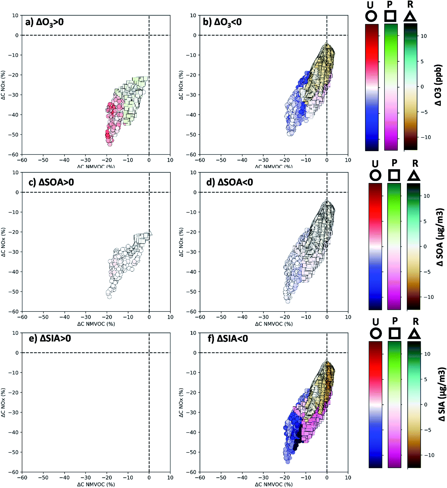 | ||
| Fig. 9 Plot of changes in daytime NOx (Y-axis) and NMVOC (X-axis) concentrations due to the lockdown (2020COVID – 2020BAU) and corresponding changes in O3 (a and b), SOA (c and d), and SIA (e and f) in all the grid cells within Urban (U), Rural (R), and Power (P) sub-regions. Results are for each sub-region (20 grid cells) during April (30 days) daytime (1000–1700 LT) hours (total data points per each sub-region are 4800). X- and Y-axes are normalized values and colors show the absolute changes. Each sub-region has a distinct color bar. The 5th layer in the model was selected to minimize the impacts of direct emissions. We did not find any increase in SIA concentrations over any of the regions; panel e does not include any data points and is blank. | ||
One shortcoming of the current analysis is that the operational WACCM global model outputs as the boundary condition in 2020 did not account for the lockdown emissions. Gaubert, et al.23 evaluated the impacts of COVID-19 lockdown on emissions and the atmospheric composition across the world using the Community Atmosphere Model with chemistry. They isolated the effect of meteorological variability and contrasted simulations with and without the daily CONFORM dataset.2 A follow-up study focused specifically on the impact of the pandemic and the natural variability on free tropospheric ozone anomalies in 2020.75 In their study, Sim.1 refers to a control scenario and Sim. 6 refers to a scenario with surface and aircraft emissions adjusted for the COVID-19 lockdown accompanied by an enhanced stratospheric denitrification rate following recommendation from Wilka, et al.76 We performed an experiment using the results of these two simulations89 as the boundary condition for our model (other inputs were the same as the 2020COVID scenario). Our results showed that the transboundary COVID-19 lockdown measures also affected the air quality over India (Fig. S18†). In particular, SIA2.5 (primarily sulfate aerosols), CO, and ozone concentrations decreased while PA2.5 slightly increased over the western parts of the domain, primarily due to the dominance of rural parts outside the boundary and increased OC emissions in some parts of the world.2,23 While taking into account the impacts of lockdown in boundary conditions improve the representation of ozone, the impacts remain small at the surface.
To better illustrate the response of air quality to changes in NOx and NMVOC concentrations, we show the response of the model in all the grid cells in Urban, Rural, and Power sub-regions to the lockdown emission changes during all daytime hours in April (Fig. 9). Ozone was the only pollutant that showed relatively large increases due to significant reductions in NOx and NMVOC concentrations. Most of these increasing ozone data points belong to only four (out of 20) grid cells located in the eastern part of the Urban sub-region (not shown). This part of Urban has the highest population density and the highest NOx emissions (i.e. eastern Delhi). The largest increases were observed at NOx reductions of more than 30%. While the Urban sub-region showed enhancements, the ozone concentration didn't increase in Rural (and a few grid cells showed less than 1 ppb increase in Power). On the other hand, ozone reduction absolute magnitudes were larger in Urban (up to 9 ppb) compared to other sub-regions (up to 6 and 5 ppb in Rural and Power, respectively). However, it should be noted that the largest average reduction in percentages belonged to Rural (Table S7†). We also looked at the changes in SOA and SIA, in which the model showed no enhancements in any sub-region. However, larger reductions for SIA (up to 19 μg m−3) than SOA (up to 2 μg m−3) were modeled. Furthermore, the Urban sub-region showed larger absolute reductions compared with Rural and Power, as was shown for ozone. Regarding the changes in NMVOC and NOx concentrations, daytime NMVOC and NOx concentrations decreased up to 20% and 50%, respectively, in Urban, while smaller reductions were found in Rural and Power. This is because Rural and Power had much lower anthropogenic emissions that could be impacted by COVID-19 lockdown perturbations. These analyses show that reducing NOx and NMVOC emissions has large potential to reduce secondary aerosol concentrations everywhere in India. In particular, less NOx could form less nitrate aerosol.71,77 However, emission reductions may lead to enhanced ozone due to its complex chemical process in urban areas and this increased oxidizing capacity could increase SOA concentrations as shown in Fig. 9c and other studies.71,77
Process analysis of ozone chemistry
As presented in the previous section, the changes in ozone concentrations did not exactly follow the changes in its precursors' emissions during the lockdown period. Specifically, NOx and VOCs anthropogenic emissions were significantly decreased as a response to the lockdown in India by up to 30% (Fig. 2), whereas daytime ozone concentrations showed only a 4% reduction (Fig. 8). More interestingly, 24-hour averaged ozone mixing ratios were higher on some days over Delhi during the lockdown period compared with the pre-lockdown period (Fig. S7†). In this section, we utilize the model outputs and IRR capability of the WRF-Chem model to study the chemistry of ozone. Fig. 10 shows the surface ozone mixing ratio and planetary boundary layer height (PBLH) averaged within Urban, Power, and Rural regions for pre-lockdown (13 March) and lockdown (7 April) days (Fig. S19† shows a similar plot for longer periods). First, we analyze the pre-lockdown day in Fig. 10 (left column). It shows that the differences within each region were only because of meteorology (2019 vs. 2020). In Urban, the evolution of the planetary boundary layer (PBL) was similar for both 2019 and 2020 scenarios and ozone followed a similar trend as the PBL, with the peak at 1530 LT. In Power, the PBLH was lower in 2020 (1 km) compared with 2019 (3 km), which is consistent with this day's lower temperature and higher wind speed in 2020 (Fig. S17†). However, ozone mixing ratios were close to each other although peaking at different hours (1530 LT in 2019 vs. 1130 LT in 2020). Similarly in Rural, models showed different PBL evolution, while the ozone mixing ratio showed a smooth similar pattern between 2019 and 2020. The reason that lower modeled PBLH of 2020, compared with 2019, in Power and Rural did not necessarily lead to a higher ozone mixing ratio is that both atmospheric dynamics and chemistry are important in the modeled ozone concentration.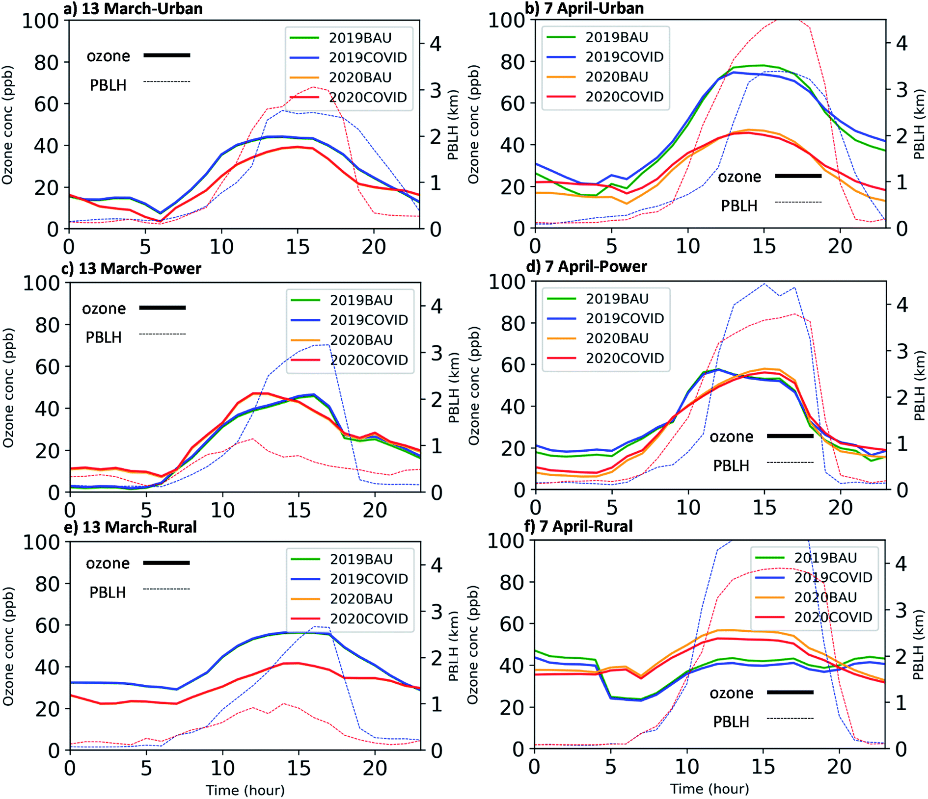 | ||
| Fig. 10 Surface ozone mixing ratio (primary Y-axis) and PBLH (secondary Y-axis) averaged over Urban (top row), Power (middle row), and Rural (bottom row) for a sampled pre-lockdown day (13 March: left column) and lockdown day (7 April: right column). In each sub-plot, the ozone concentration is shown with a solid line and PBLH is shown with a dotted line (blue for 2019, red for 2020). The results are shown for all the scenarios: 2019BAU (green), 2019COVID (blue), 2020BAU (orange), and 2020COVID (red). | ||
Second, we analyze the lockdown day (7 April) in Fig. 10 (right column). In Delhi, the PBL grew faster and extended higher in 2020, while both years peaked during afternoon hours. The shallower PBLH in 2019 means more precursors are available in the shallower atmosphere (i.e. less dilution), leading to more ozone formation during the day. Furthermore, background ozone also affects the ozone concentrations as discussed before. In addition, the model simulated higher CO concentrations over the IGP in 2019 which could lead to more ozone formation (not shown). Srinivas, et al.78 found that transported pollution from the Bay of Bengal can potentially elevate the CO concentrations in Delhi. We are also interested in the impacts of lockdown emission. Comparing 2020BAU and 2020COVID, the lockdown resulted in a slightly lower peak value. It should be emphasized that this was not the case for all the days during the lockdown period as the impact of emissions on daytime ozone mixing ratio varied day by day in Urban (Fig. 6). On the other hand, the largest difference in the ozone mixing ratio happens during 0030–0730 LT and 1830–2330 LT. While the reaction between NO and ozone could deplete all the ozone in the atmosphere, the titration did not deplete all the ozone in the 2020COVID scenario due to lower amounts of NO available. As a result, more residual ozone remained in the atmosphere. In particular, panels b and d show more nighttime ozone during the nighttime in Urban and Power, respectively. Ciarelli, et al.71 also found a similar trend of nighttime ozone increase over northern Italy and Switzerland, which led to a daily ozone increase. However, the daytime ozone decreased both in the current study and that reported in ref. 71.
In Power, the PBL grew faster in 2020 but its peak height was lower than that in 2019. However, the daytime ozone mixing ratios did not change between both years (although the morning time (0830–1030 LT) ozone was higher in 2019 due to lower PBLH). We also observed small changes between 2020BAU and 2020COVID scenarios. Although the percentage of emission changes was large for both VOCs and NOx, the amount of anthropogenic VOC emissions was low in this region and NOx emissions in Power were even more than in Urban (Table S3†). Furthermore, the eastern IGP was also significantly impacted by biogenic emissions on 7 April 2020 (Fig. S17†). As a result, biogenic VOC emissions controlled the ozone formation, which were similar in both 2020BAU and 2020COVID scenarios.
In Rural, the PBL growth in 2019 was faster and it extended higher than that in 2020. Fig. S17† also shows that the wind speed in Rural was lower by ∼75% on 7 April 2020 compared with the same day in 2019, leaning towards a stagnant condition. As a result, the ozone mixing ratio is higher in 2020 scenarios. Comparing 2020BAU and 2020COVID shows a reduction during all hours due to the lockdown emissions.
OH reactivity
Fig. 11 shows the OH reactivity with VOCs and NO2 within Urban, Power, and Rural regions for a pre-lockdown (13 March) and lockdown (7 April) day (Fig. S20† shows a similar plot for longer periods). We followed Pfister, et al.30 suggestion in averaging these values within the PBL to minimize the effects of mixing. It is important to note (1) these OH reactivity plots are averaged within the PBL, while ozone mixing ratios in Fig. 10 were surface values and (2) these plots indicate the chemistry contribution to the ozone mixing ratio, while other contributing factors such as vertical mixing and advection are also important processes impacting the actual ozone mixing ratio.48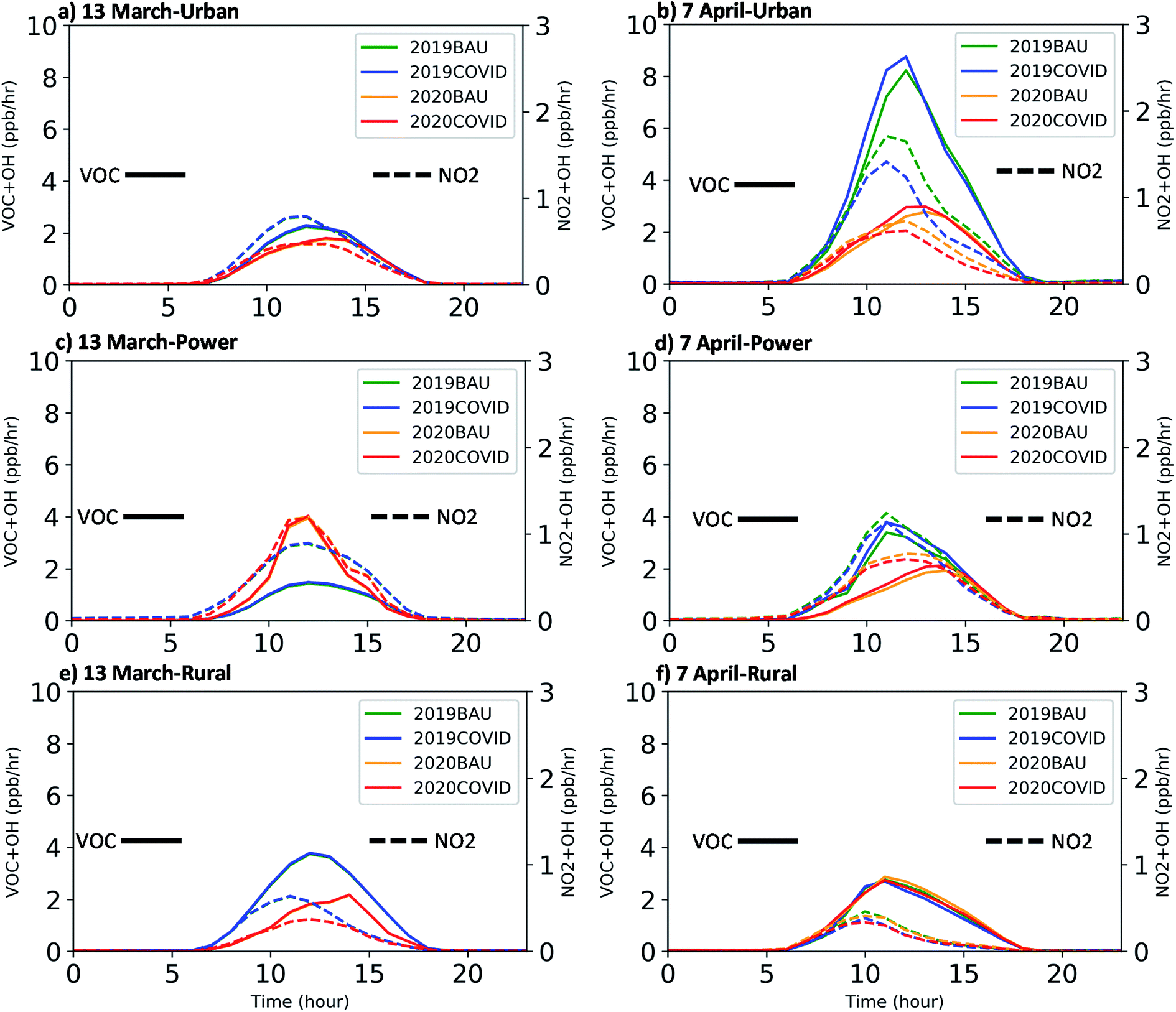 | ||
| Fig. 11 OH reactivity with VOCs (primary Y-axis) and NO2 (secondary Y-axis) averaged within PBL over Urban (top row), Power (middle row), and Rural (bottom row) for a sampled pre-lockdown day (13 March: left column) and lockdown day (7 April: right column). In each sub-plot, OH reactivity with VOCs and NO2 is shown with solid and dashed lines, respectively. The results are shown for all the scenarios: 2019BAU (green), 2019COVID (blue), 2020BAU (orange), and 2020COVID (red). | ||
During the pre-lockdown day, VOC + OH and NO2 + OH were different for 2019 and 2020 in Urban. Although there were also some differences in the time of the peaks, the ratio of VOC + OH to NO2 + OH was similar, suggesting that the ozone formation was not very much different. In Power, both VOC + OH and NO2 + OH increased in 2020 but to different extents. The peak VOC + OH increased by 4 times while NO2 + OH increased by two times. In Power, the anthropogenic NOx emissions are higher than natural emissions. Therefore, changing the meteorology (i.e. more biogenic VOC emissions in 2020) increases the rate of both reactions. In Rural, the results showed smaller VOC + OH rates in 2020 with roughly similar NO2 + OH rates. However, both VOC and NOx anthropogenic emissions were low in this region and very similar between 2019 and 2020. Similarly, it indicates the importance of meteorology effects and accompanying biogenic and biomass burning emissions on the ozone formation in Rural.
During the lockdown day, OH reactivity (with both VOC and NO2) was higher in 2019 scenarios than 2020 in Urban. This is consistent with shallower PBL in 2019, which led to higher ozone mixing ratios. In other words, it shows that the effect of meteorology on observed air pollution could be significant on some days. In addition, the effect of lockdown emissions on ozone production and destruction was low in both 2019 and 2020. In 2020 scenarios, there was a drop and rise due to lockdown emissions in NO2 + OH and VOC + OH, respectively. Ciarelli, et al.71 showed a similar response over an urban region (i.e. Milan, Italy). Nevertheless, the daytime surface ozone concentration did not increase in the 2020COVID scenario (Fig. 10b). This indicates the complexity of ozone formation and the importance of both HOx and NOx cycles within this process. Although we saw large reductions in NOx emissions in Urban, there was also a reduction in VOCs, which resulted in a small shift in the ozone formation process (Table S10†).
In Power, larger OH reactivity values were observed for both VOC and NO2 in 2019 compared with 2020 in both anthropogenic emission scenarios (i.e. 2019BAU vs. 2020BAU or 2019COVID vs. 2020COVID). These larger values in 2019 scenarios were unexpected since anthropogenic emissions were similar in each of these comparisons and we observed larger biogenic isoprene emissions on 7 April 2020 (Fig. S17†). However, this can be explained by higher CO contribution in 2019 results (Fig. S25†). On the other hand, the biogenic soil NO emission was also larger in 2019, resulting in more ozone formation. Considering the lockdown emissions, the model showed that the adjusted emissions (i.e. COVID scenarios) did not change VOC + OH values very much. This is due to low anthropogenic and equal biogenic VOC emissions in this region.
In Rural, we observed similar behaviour of OH reactivity for both 2019 and 2020. This is consistent with a similar ozone mixing ratio trend in Fig. 10. As emissions are low in this region, ozone formation and OH reactivity do not play an important role and ozone differences can be explained by dynamics and atmospheric stability. As a result, adjusted emissions had a negligible and similar effect on both VOC + OH and NO2 + OH rates in 2020 scenarios.
Comparing the total OH consumed by each pathway (i.e. integrating the 24 h values in Fig. 11 for 7 April as the lockdown day) and their ratio in 2020BAU and 2020COVID scenarios can also provide some information on whether the ozone chemistry regime changed because of the lockdown. Table S10† shows that the integrated values in total OH consumption by VOCs were higher in Urban and Rural compared with Power, confirming lower VOCs in the Power region. Moreover, the ratio of total OH consumption by VOC to NO2 had the largest values in Rural, showing low NO2 available in this region. Evaluating the change of the ratio because of lockdown emissions suggests that Urban and Rural shifted toward the NOx limited regime, while the ozone chemistry regime did not change in Power.
FNR and VOC/NOX sensitivities
As discussed earlier, LROx and LNOx are the reactions that determine the radical terminations by radicals and NOx, respectively, during the daytime (Tables S8 and S9†). More information on the IRR analysis methodology is provided in the ESI.† The LROx/LNOx ratio is very important from a policy perspective as it indicates whether reduction in NOx (large ratio values; i.e. NOx-limited) or VOC (small ratio values; i.e. VOC-limited) emission is the efficient strategy for ozone reduction. Duncan, et al.79 assumed that the transition between NOx-limited and VOC-limited regions happens at a LROx/LNOx ratio of one. Schroeder, et al.80 found that the transition of ozone production occurs at a ratio of 0.35 using 0-D photochemical box modeling. However, evaluating the LROx and LNOx values is not usually possible based on observations. As a result Sillman81 proposed using the ratio of measured tracers in the atmosphere as an alternative. The formaldehyde to NO2 ratio (FNR) is one of the most frequently used ratios as its species can be measured from both ground measurements and space borne instruments.16,82,83 However, characterization of the FNR range is important to estimate the chemical regime. Mahajan, et al.84 used the FNR transition range between one and two to study the inter-annual variations of ozone formation in India using satellite observations, whereas Schroeder, et al.80 showed that this transition range is not constant in all regions. For example, they found in their box modeling study in the US that the transition range was 0.9–1.80 in Colorado, while the range of 0.7–2.0 was found for Houston, Texas. In other words, the FNR transition range for each region should be exclusively specified for each region. In the following analysis, we use the LROX and LNOX, and FNR information from the model to study the ozone chemical regimes in each grid cell in northern India. We classify each grid cell as an urban, rural, or a power plant region (more information on the classification process can be found in the ESI†). Furthermore, all the days in April are included in this analysis.Fig. 12 shows the plots of the FNR within the PBL as a function of LROx/LNOx in all the urban, rural, and power-plant grid cells for the 2019BAU, 2020BAU, and 2020COVID scenarios during the afternoon hours (1230–1430 LT) for all the days in April. Comparing the results for 2019BAU and 2020BAU suggests that meteorological differences within the years do not change the chemical regime in a region in a short period. For example, the 2019BAU scenario showed that 28% of urban grid cells were in the VOC-limited region (i.e. LROx/LNOx < 0.35) and this number was 25% for the 2020BAU scenario. However, comparing the results for different regions within one scenario shows that the ozone formation regime differs for each region. In particular, the results for the 2019BAU scenario show that 25% of the power-plant grid cells were in the VOC-limited regime, whereas only 6% of the rural grid cells were in the VOC-limited regime. These results indicate that we cannot employ one uniform emission control strategy everywhere. We also identified the results for the Urban, Rural, and Power regions (green points in Fig. 12). The results for Urban, which primarily covers Delhi, showed that 81% of points were in the VOC-limited regime in the 2019BAU scenario. This supports the idea that the emission control strategies that target the transportation sector (i.e. NOx emission), with the primary goal of PM reduction, can increase ozone.26 In Power, 76% (77%) of the points in 2019BAU (2020BAU) were in the VOC-limited region, which is expected as this domain had low amounts of anthropogenic VOC emissions (Table S3†) and biogenic emissions were the primary source of VOCs (Fig. S25†), suggesting that extreme NOx emission reduction may be the only solution in this region. While the effect of different meteorology (2019BAU vs. 2020BAU) on chemical regimes was negligible, dramatic changes in emissions can lead to large changes. For example, only 15% of urban grid cells were in the VOC-limited regime in the 2020COVID scenario, in which both NMVOC and NOx emissions had large reductions.
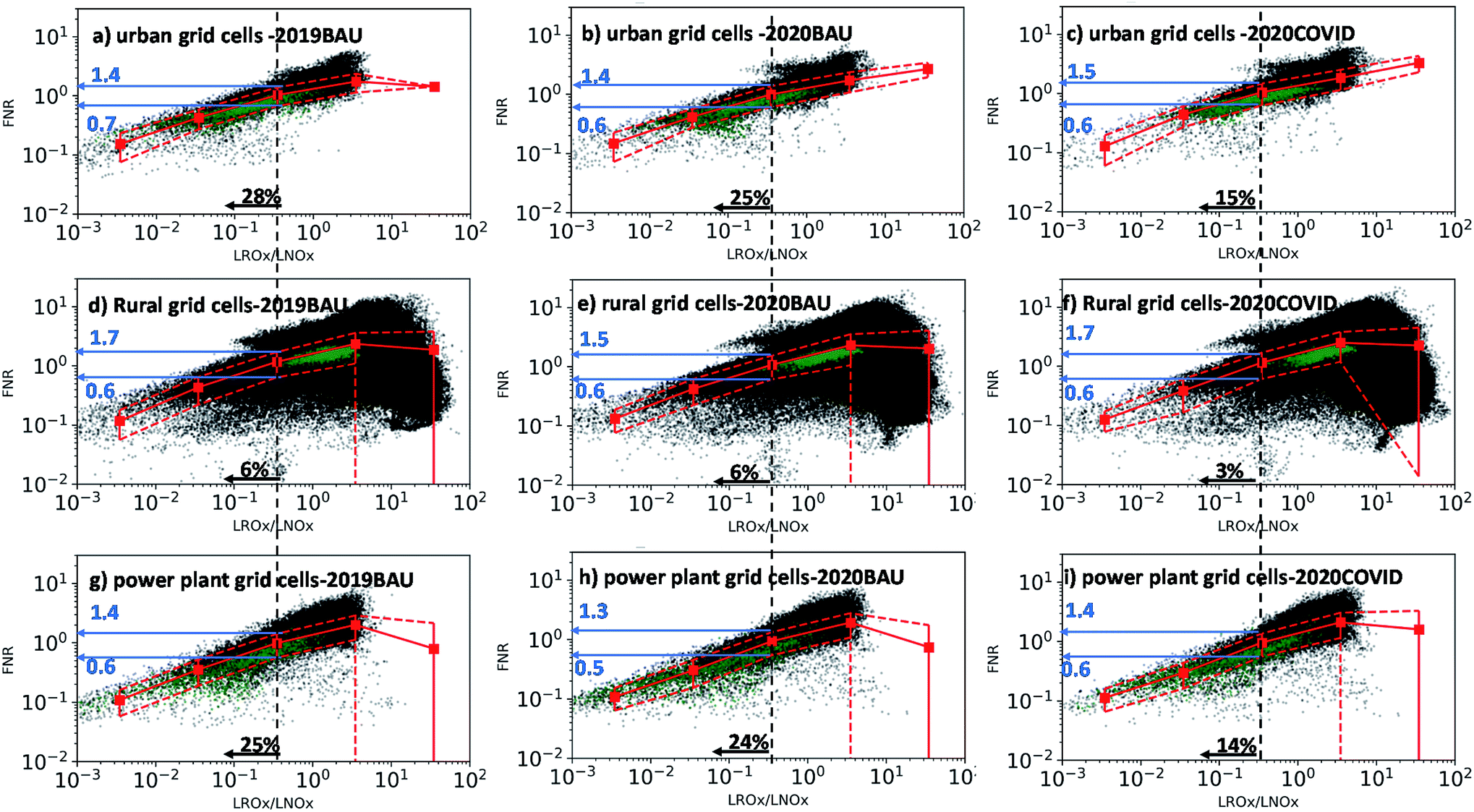 | ||
| Fig. 12 Plots of the point-to-point FNR (within the PBL) as a function of the LROx/LNOx ratio during afternoon hours (1230–1430 LT) for 2019BAU (left column), 2020BAU (middle column), and 2020COVID (right column) scenarios in all urban (a–c), rural (d–f), and power plant (g–i) grid cells in northern India for all the days in April. Black points show all the grid cells within each category and green points show the grid cells in predefined Urban, Rural, and Power regions. Five bins were assumed and binned averages (red squares) and standard deviations (vertical red solid bars) were calculated. The vertical dashed black line represents the LROx/LNOx ratio of 0.35 (overlaid on bin 3 median). The percentage of the points that were in the VOC-limited regime (LROx/LNOx < 0.35) is shown in black in each subpanel. The horizontal blue vectors show the corresponding FNR transition range in each region (numbers in blue show the values). | ||
Calculating binned averages and corresponding standard deviations for the FNR data can provide some insights about the transition range.80 As discussed above, the meteorology effects were small. As a result, we took the union of the transition range of 2019BAU and 2020BAU scenarios to minimize the effect of meteorology. In urban grid cells, our results suggest that the FNR transition range is 0.6–1.4. Lee, et al.85 studied FNR values in nine megacities in East Asia and suggested the ozone chemical regime to be NOx-saturated when the FNR is below 1.5. In rural grid cells, the union of the FNR transition range, for 2019BAU and 2020BAU scenarios, is 0.6–1.7. In other words, the FNR transition range is wider in the rural regions compared with the urban regions. In the power-plant grid cells, the union FNR transition range is 0.5–1.4. On the other hand, large NOx and NMVOC emission reductions during the COVID19 lockdown period (i.e. 2020COVID) slightly changed the FNR. Furthermore, it shifted the FNR transition range in some regions. The percentage of grid cells within FNR transition range in each scenario and region is provided in Table S11.†Fig. 13 shows the spatial changes in the ozone chemical regime due to COVID19 lockdown emissions over the domain using the FNR analysis. The results for the 2020BAU scenario show that the FNR in most parts of northern India was larger than the highest estimated upper-limit of FNR transition ranges (i.e. 1.7 in the rural grid cells in the 2020COVID scenario), indicating that they are in the NOx-limited regime. Indeed, all the regions other than most parts of the IGP and power plant regions fall in the NOx-limited regime. The colour over most parts of the IGP is green suggesting that their VOC-limited regime is close to transition and can potentially shift to a VOC-limited regime depending on the future urban developments in this region. On the other hand, the FNR was very low in some places like Delhi and the Power region, showing that the chemical regime continues to remain as VOC-limited. The lockdown emissions (2020COVID) revealed that the FNR increased over the domain, moving most parts of the western and eastern IGP to warmer colours; i.e. the NOx-limited regime. However, the FNR in some urban locations (e.g. Delhi) and the Power region remained low; the ozone production regime did not change as was expected. Overall, our analysis indicate that the FNR can determine a region that is strictly NOx- or VOC-limited (e.g. Power) but caution should be exercised for regions close to the defined transition regions (e.g. most parts of the IGP). Compared to the FNR retrieved from TROPOMI retrievals (Fig. S10†), the model overestimated the amount of reduction between April 2019 and 2020 although captured the overall regional changes over most parts of the domain. We also found lower absolute FNR values in both April 2019 and 2020 (not shown). Other studies have also reported a biased low modeled FNR over India.84 This can be due in part to the model underestimation of formaldehyde86 and the calculation of the air mass factor in the satellite data.87 Furthermore, a longer period (than one month) needs to be studied for evaluating the results as future work. It should also be mentioned that while these measurable FNR estimates can be used for identifying the chemical regimes, their limitations should be kept in mind. For example, it is clear from the plots in Fig. 12 that the FNR ranges cover a large amount of data points in other bins as well, with large LROx/LNOx values. Moreover, only about 10% of the rural grid cells were in the estimated FNR transition range, increasing the uncertainty in the estimated range in the rural grid cells. Moreover, Schroeder, et al.80 emphasized that other parameters (e.g. different radicals with different lifetimes compared to formaldehyde) can affect the FNR and it may not be a solid indicator of ozone formation sensitivity in some regions. Furthermore, Souri, et al.88 studied the functionality of the FNR and found situations where LROx/LNOx and FNR lead to contradicting conclusions regarding the chemical regime in a region, primarily because of impacts of NO2 on formaldehyde.
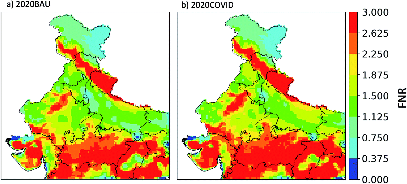 | ||
| Fig. 13 FNR (within the PBL) averaged over April using (a) 2020BAU and (b) 2020COVID scenarios. An FNR of 1.7 represents the upper limit of the transition region. | ||
Discussion
Various parameters including meteorology, base emissions, and COVID-19 lockdown emission's adjusting factors affected the observed changes in air quality over India during the lockdown period. Therefore, the uncertainty in each of these parameters could potentially lead to different findings. One parameter is the base anthropogenic emission inventory. Not only the total amount of each species but also each sector's contribution is important. In general, the total amount is important to predict the observed concentrations. Nevertheless, the sectoral contribution is also important when considering the impact of emission control scenarios. We compared our ozone formation findings with an experiment, where we replaced the CEDS_M base anthropogenic emission inventory with HTAP v2.2. As shown in Fig. S27,† the total NOx emissions over India are close together. However, the transportation sector contains 45% and 15% of total NOx in HTAP v2.2 and CEDS_M, respectively. On the other hand, the total NMVOC emissions in CEDS_M were 40% lower than HTAP v.2.2 with different contributions from the transportation sector. As a result, the effect of the COVID-19 lockdown, which largely restricted transportation, was different in these two scenarios (not shown). Fig. S23 and S24† are similar to Fig. 7 and 8, but based on HTAP v2.2. While the magnitudes of changes were different, the overall response was similar based on both emission inventories.Nevertheless, different contribution of emissions affected the insights about the ozone formation over India. IRR gives us the opportunity to find the species that have high contributions to the OH reactivity and ozone chemistry. Fig. S25 and S26† show the OH reactivity for the top six VOC species for the lockdown day in each region and the scenario based on CEDS_M and HTAP v2.2 base anthropogenic emission inventories. Both experiments show that CO was the main component in all the regions and scenarios over India. Although CO reacts slowly in the atmosphere (i.e. long lifetime), its abundant availability moves it to the top of the list. The other species were short-lived species. Formaldehyde (CH2O) was the second-ranked species in almost all the subfigures except the ones where isoprene (ISOP) had a higher reactivity rate. Specifically, ISOP was the second-ranked species in the Power region in all the scenarios. This is because VOCs in the Power region were dominated with biogenic sources and the amount of anthropogenic emissions (and their changes in COVID scenarios) did not change their rankings. ISOP was also the second-ranked species (with very close values to CH2O) in Urban for some scenarios in 2020. High contributions by CO, CH2O, and ISOP to OH reactivity are also reported in the United States.30 They found that high contribution of CH2O to OH reactivity was due to both local emissions and chemical production, while ISOP was mostly due to biogenic emissions. In this study, while CH2O had larger contribution in the Urban, ISOP had larger contributions in the Power, which is consistent with Pfister, et al.30 The contribution of other VOCs is different based on the emission inventory. For example, large alkenes (i.e. BIGALK in the model) are important VOCs based on the HTAP v2.2 inventory. In particular, they contributed to OH reactivity in the Urban region in BAU scenarios. Furthermore, they were involved in the Rural region in the 2020BAU scenario. However, they do not show up as an important VOC in the experiment using the CEDS_M inventory. By ranking the species with overall high OH reactivity based on both experiments in BAU scenarios, we identified CO, CH2O, ISOP, acetaldehyde (CH3OH), and ethylene (C2H4) as major VOCs involved in ozone formation in India.
We also evaluated the effect of the base anthropogenic emission inventory and corresponding lockdown reductions on the ozone chemical regime over India. The response was similar, showing that lockdown emissions shifted the chemistry towards the NOx-limited regime. However, CEDS_M showed more grid cells in the VOC-limited regime over India due to lower VOC emissions compared with HTAP v.2.2. In addition, the estimated FNR transition region was close though slightly different based on the inventory used. Specifically, we found the union of the FNR transition region of 0.4–1.9 using HTAP v2.2 in contrast with 0.5–1.7 using the CEDS_M inventory. This shows that our analysis was robust and the accuracy of emission inventories had small effects on the findings. Nevertheless, the sector contributions in the studied inventories had large uncertainties. In general, these comparisons suggest that while the insights are roughly similar, the action points can be different based on the accuracy of the base emission inventory.
Summary and conclusion
We studied the contributions of inter-annual variability in meteorology and emissions (dust, biogenic, and biomass burning) and COVID-19 lockdown emissions to northern India's air quality and explored the chemistry behind the changes in ozone concentrations. For this purpose, we used the WRF-Chem version 4.0 model to utilize its integrated reaction rate (IRR) capability. The adjustment factors proposed by Doumbia, et al.2 were used to account for the anthropogenic emission changes during the lockdown period in India. The model was able to capture the overall observed trend in air pollutant concentrations in 2019 and 2020.Four scenarios were designed to study the effect of the meteorology and lockdown anthropogenic emission perturbations in April 2019 and 2020. We found that the effects of perturbing the anthropogenic emissions could be different depending on the applied year. The reason is that not only the anthropogenic emissions but also the meteorological dependent emissions (e.g. biogenic emissions) and the atmospheric dynamics affect the air quality in a region. We also estimated the changes in air pollutant concentrations between April 2019 and 2020 and the contribution of meteorology and lockdown emissions. While the PM2.5 concentration averaged over the IGP decreased by 12% in April 2020 due to the meteorology, it increased in central India due to more biomass burning emissions. However, the lockdown emissions decreased the PM2.5 concentration over Indian parts of the domain by 9%. For ozone, we found that meteorology decreased the concentrations over the IGP and increased them over central India, similar to PM2.5. However, the ozone concentration response to significant reductions in its precursors (i.e. NO2 and VOCs) due to the lockdown emissions was not constant over the domain. While ozone decreased in most parts of the domain, we saw that major cities like Delhi and the regions with many power plants showed slight increases in ozone with decreases in NOx emissions.
We also analyzed the ozone chemistry in an urban, a rural, and a densely populated power plant region during a sampled pre-lockdown and lockdown day. Using OH reactivity with VOCs (NO2) as the pathway to ozone formation (destruction), we found that the lockdown emissions decreased both pathways in the urban and rural regions. However, it only decreased the ozone destruction in the power plant region (NO2 + OH) and did not affect the ozone formation path (VOC + OH), as natural emission sources dominated the VOC emissions in this region.
Furthermore, we calculated the rates that radicals (i.e. HO2 and RO2) react with radicals (i.e. LROx) or NO2 (i.e. LNOx) and used their ratio (LROx/LNOx) to find the ozone chemistry regime in different regions. Our analysis showed that there were more VOC-limited grid cells in urban and power plant regions (LROx/LNOx < 0.35) compared with the rural regions, which were mainly in a NOx-limited regime. Following Schroeder, et al.,80 we also calculated this ratio's corresponding formaldehyde to NO2 concentration ratio (FNR) in each region. In general, this is preferred as it can be calculated using ground measurements and satellite observation data. Our analysis suggested the FNR of 1.7 as the upper-limit of the transition regime from VOC-limited to NOx-limited over northern India. Using this threshold, we classified most parts of India in the NOx-limited regime while most parts of the IGP and power plant region were in the VOC-limited regime.
We also investigated the effect of the base anthropogenic emission inventory on our findings. We found that the qualitative response of the model did not change based on the emission inventory. However, the details were different, leading to different insights into ozone formation. Overall, we identified CO, formaldehyde, isoprene, acetaldehyde, and ethylene as the major VOCs contributing to the ozone formation over India.
Understanding the ozone formation chemistry and the role of emission sources and different species can help the policy makers to implement efficient emission control scenarios. Our results showed that the ozone formation process could be different in each region depending on its local anthropogenic and natural emission sources and the meteorology. Our findings also revealed that air pollution management strategies should consider both PM2.5 and ozone pollutants and include emission controls for both NOx and VOC emissions. While our results can provide information on the overall response of the air quality to emission reductions, they do not necessarily represent the general ozone chemistry in India, as we showed distinct behaviour in different regions. However, it provides a framework that can be used to study the efficacy of local emission control scenarios on ozone formation in India. Moreover, the findings of this study show that while top-down techniques can be extremely useful for developing emission inventories, bottom-up sectoral emission inventories are still a critical body of information in identifying the action points for improving the air quality.
Author contributions
BR and GRC designed the research; BR performed all the model simulations; SKG provided the measurement data; BR and MAO analyzed the IRR outputs. BR and GRC wrote the paper. All authors contributed to discussion and edited the paper.Conflicts of interest
The authors declare that they have no conflict of interest.Acknowledgements
This work was funded in part by NASA HAQAST and ACMAP projects under awards NNX16AQ19G and 80NSSC19K094, respectively. BR also acknowledges support from the University of Iowa graduate college summer fellowship. All the calculations and simulations were done using the University of Iowa's Argon high-performance computing cluster. The WRF-Chem and IRR hourly output results for all four scenarios are available from Iowa Research Online at https://doi.org/10.25820/data.006144. TROPOMI data can be freely downloaded from the European Space Agency Copernicus Open Access Hub (https://doi.org/10.5270/S5P-s4ljg54). MERRA-2 data can be freely downloaded from NASA EarthData Portal (https://earthdata.nasa.gov/). We thank Dr Benjamin Gaubert, NCAR for providing his model outputs that were used for boundary condition as part of this study. We also thank Dr Louisa Emmons, NCAR for providing VOC speciation between the emission inventory and model inputs.References
- M. E. Gorris, S. C. Anenberg, D. L. Goldberg, G. H. Kerr, J. D. Stowell, D. Tong and B. F. Zaitchik, Shaping the future of science: COVID-19 highlighting the importance of GeoHealth GeoHealth, 2021, 5, e2021GH000412, DOI:10.1029/2021GH000412.
- T. Doumbia, C. Granier, N. Elguindi, I. Bouarar, S. Darras, G. Brasseur, B. Gaubert, Y. Liu, X. Shi and T. Stavrakou, Changes in global air pollutant emissions during the COVID-19 pandemic: a dataset for atmospheric chemistry modeling, Earth Syst. Sci. Data, 2021, 13, 4191–4206, DOI:10.5194/essd-13-4191-2021.
- M. Amann, G. Kiesewetter, W. Schöpp, Z. Klimont, W. Winiwarter, J. Cofala, P. Rafaj, L. Höglund-Isaksson, A. Gomez-Sabriana and C. Heyes, Reducing global air pollution: the scope for further policy interventions, Philos. Trans. R. Soc., A, 2020, 378, 20190331, DOI:10.1098/rsta.2019.0331.
- G. I. Gkatzelis, J. B. Gilman, S. S. Brown, H. Eskes, A. R. Gomes, A. C. Lange, B. C. McDonald, J. Peischl, A. Petzold, C. R. Thompson and A. Kiendler-Scharr, The global impacts of COVID-19 lockdowns on urban air pollution: A critical review and recommendations, Elementa: Science of the Anthropocene, 2021, 9(1), 00176, DOI:10.1525/elementa.2021.00176.
- R. S. Sokhi, V. Singh, X. Querol, S. Finardi, A. C. Targino, M. d. F. Andrade, R. Pavlovic, R. M. Garland, J. Massagué, S. Kong, A. Baklanov, L. Ren, O. Tarasova, G. Carmichael, V.-H. Peuch, V. Anand, G. Arbilla, K. Badali, G. Beig, L. C. Belalcazar, A. Bolignano, P. Brimblecombe, P. Camacho, A. Casallas, J.-P. Charland, J. Choi, E. Chourdakis, I. Coll, M. Collins, J. Cyrys, C. M. da Silva, A. D. Di Giosa, A. Di Leo, C. Ferro, M. Gavidia-Calderon, A. Gayen, A. Ginzburg, F. Godefroy, Y. A. Gonzalez, M. Guevara-Luna, S. M. Haque, H. Havenga, D. Herod, U. Hõrrak, T. Hussein, S. Ibarra, M. Jaimes, M. Kaasik, R. Khaiwal, J. Kim, A. Kousa, J. Kukkonen, M. Kulmala, J. Kuula, N. La Violette, G. Lanzani, X. Liu, S. MacDougall, P. M. Manseau, G. Marchegiani, B. McDonald, S. V. Mishra, L. T. Molina, D. Mooibroek, S. Mor, N. Moussiopoulos, F. Murena, J. V. Niemi, S. Noe, T. Nogueira, M. Norman, J. L. Pérez-Camaño, T. Petäjä, S. Piketh, A. Rathod, K. Reid, A. Retama, O. Rivera, N. Y. Rojas, J. P. Rojas-Quincho, R. San José, O. Sánchez, R. J. Seguel, S. Sillanpää, Y. Su, N. Tapper, A. Terrazas, H. Timonen, D. Toscano, G. Tsegas, G. J. M. Velders, C. Vlachokostas, E. von Schneidemesser, R. Vpm, R. Yadav, R. Zalakeviciute and M. Zavala, A global observational analysis to understand changes in air quality during exceptionally low anthropogenic emission conditions, Environ. Int., 2021, 157, 106818, DOI:10.1016/j.envint.2021.106818.
- S. D. Ghude, C. Jena, D. Chate, G. Beig, G. Pfister, R. Kumar and V. Ramanathan, Reductions in India’s crop yield due to ozone, Geophys. Res. Lett., 2014, 41, 5685–5691, DOI:10.1002/2014GL060930.
- HEI, Burden of Disease Attributable to Major Air Pollution Sources in India, 2018 Search PubMed.
- B. Roozitalab, G. R. Carmichael and S. K. Guttikunda, Improving regional air quality predictions in the Indo-Gangetic Plain–case study of an intensive pollution episode in November 2017, Atmos. Chem. Phys., 2021, 21, 2837–2860, DOI:10.5194/acp-21-2837-2021.
- S. Gupta, Air pollution in northern India has hit a 20-year low, NASA report says, 2020, https://www.cnn.com/2020/04/23/india/india-air-pollution-coronavirus-nasa-intl/index.html.
- G. Beig, N. Korhale, A. Rathod, S. Maji, S. K. Sahu, S. Dole, R. Latha and B. Murthy, On modelling growing menace of household emissions under COVID-19 in Indian metros, Environ. Pollut., 2021, 272, 115993, DOI:10.1016/j.envpol.2020.115993.
- D. L. Goldberg, P. E. Saide, L. N. Lamsal, B. d. Foy, Z. Lu, J.-H. Woo, Y. Kim, J. Kim, M. Gao and G. Carmichael, A top-down assessment using OMI NO 2 suggests an underestimate in the NOx emissions inventory in Seoul, South Korea, during KORUS-AQ, Atmos. Chem. Phys., 2019, 19, 1801–1818, DOI:10.5194/acp-19-1801-2019.
- ESA, Air pollution drops in India following lockdown, https://www.esa.int/Applications/Observing_the_Earth/Copernicus/Sentinel-5P/Air_pollution_drops_in_India_following_lockdown#.YFzj-71W1ss.link, accessed 03/25/2021, 2021 Search PubMed.
- A. Biswal, V. Singh, S. Singh, A. P. Kesarkar, K. Ravindra, R. S. Sokhi, M. P. Chipperfield, S. S. Dhomse, R. J. Pope and T. Singh, COVID-19 lockdown induced changes in NO 2 levels across India observed by multi-satellite and surface observations, Atmos. Chem. Phys. Discuss., 2020, 1–28, DOI:10.5194/acp-21-5235-2021.
- A. Siddiqui, S. Halder, P. Chauhan and P. Kumar, COVID-19 Pandemic and City-Level Nitrogen Dioxide (NO2) Reduction for Urban Centres of India, J. Indian Soc. Remote Sens., 2020, 48, 999–1006, DOI:10.1007/s12524-020-01130-7.
- S. Jain and T. Sharma, Social and travel lockdown impact considering coronavirus disease (COVID-19) on air quality in megacities of India: Present benefits, future challenges and way forward, Aerosol Air Qual. Res., 2020, 20, 1222–1236, DOI:10.4209/aaqr.2020.04.0171.
- V. Kumar, S. Beirle, S. Dörner, A. K. Mishra, S. Donner, Y. Wang, V. Sinha and T. Wagner, Long-term MAX-DOAS measurements of NO 2, HCHO, and aerosols and evaluation of corresponding satellite data products over Mohali in the Indo-Gangetic Plain, Atmos. Chem. Phys., 2020, 20, 14183–14235, DOI:10.5194/acp-20-14183-2020.
- P. Kumari and D. Toshniwal, Impact of lockdown measures during COVID-19 on air quality–A case study of India, Int. J. Environ. Health Res., 2020, 1–8, DOI:10.1080/09603123.2020.1778646.
- S. Mahato, S. Pal and K. G. Ghosh, Effect of lockdown amid COVID-19 pandemic on air quality of the megacity Delhi, India, Sci. Total Environ., 2020, 730, 139086, DOI:10.1016/j.scitotenv.2020.139086.
- S. Selvam, P. Muthukumar, S. Venkatramanan, P. Roy, K. M. Bharath and K. Jesuraja, SARS-CoV-2 pandemic lockdown: effects on air quality in the industrialized Gujarat state of India, Sci. Total Environ., 2020, 737, 140391, DOI:10.1016/j.scitotenv.2020.140391.
- V. Singh, S. Singh, A. Biswal, A. P. Kesarkar, S. Mor and K. Ravindra, Diurnal and temporal changes in air pollution during COVID-19 strict lockdown over different regions of India, Environ. Pollut., 2020, 266, 115368, DOI:10.1016/j.envpol.2020.115368.
- M. Zhang, A. Katiyar, S. Zhu, J. Shen, M. Xia, J. Ma, S. H. Kota, P. Wang and H. Zhang, Impact of reduced anthropogenic emissions during COVID-19 on air quality in India, Atmos. Chem. Phys., 2021, 21, 4025–4037, DOI:10.5194/acp-21-4025-2021.
- U. Dumka, D. Kaskaoutis, S. Verma, S. S. Ningombam, S. Kumar and S. Ghosh, Silver linings in the dark clouds of COVID-19: Improvement of air quality over India and Delhi metropolitan area from measurements and WRF-CHIMERE model simulations, Atmos. Pollut. Res., 2021, 12, 225–242, DOI:10.1016/j.apr.2020.11.005.
- B. Gaubert, I. Bouarar, T. Doumbia, Y. Liu, T. Stavrakou, A. M. Deroubaix, S. Darras, N. Elguindi, C. Granier and F. G. Lacey, Global Changes in Secondary Atmospheric Pollutants during the 2020 COVID-19 Pandemic, J. Geophys. Res.: Atmos., 2020, 126, e2020JD034213, DOI:10.1029/2020JD034213.
- K. Miyazaki, K. Bowman, T. Sekiya, M. Takigawa, J. L. Neu, K. Sudo, G. Osterman and H. Eskes, Global Tropospheric Ozone Responses to Reduced NOx Emissions Linked to the COVID-19 World-Wide Lockdowns Sci. Adv., 2021, 7(24), eabf7460, DOI:10.1126/sciadv.abf7460.
- S. Mor, S. Kumar, T. Singh, S. Dogra, V. Pandey and K. Ravindra, Impact of COVID-19 lockdown on air quality in Chandigarh, India: understanding the emission sources during controlled anthropogenic activities, Chemosphere, 2021, 263, 127978, DOI:10.1016/j.chemosphere.2020.127978.
- Y. Chen, G. Beig, S. Archer-Nicholls, W. Drysdale, W. J. F. Acton, D. Lowe, B. Nelson, J. Lee, L. Ran and Y. Wang, Avoiding high ozone pollution in Delhi, India, Faraday Discuss., 2020, 226, 502–514, 10.1039/D0FD00079E.
- M. Tzortziou, C. F. Kwong, D. Goldberg, L. Schiferl, R. Commane, N. Abuhassan, J. J. Szykman and L. C. Valin, Declines and peaks in NO2 pollution during the multiple waves of the COVID-19 pandemic in the New York metropolitan area, Atmos. Chem. Phys., 2022, 22, 2399–2417, DOI:10.5194/acp-22-2399-2022.
- D. L. Goldberg, S. C. Anenberg, D. Griffin, C. A. McLinden, Z. Lu and D. G. Streets, Disentangling the impact of the COVID-19 lockdowns on urban NO2 from natural variability, Geophys. Res. Lett., 2020, 47, e2020GL089269, DOI:10.1029/2020GL089269.
- G. A. Grell, S. E. Peckham, R. Schmitz, S. A. McKeen, G. Frost, W. C. Skamarock and B. Eder, Fully coupled “online” chemistry within the WRF model, Atmos. Environ., 2005, 39, 6957–6975, DOI:10.1016/j.atmosenv.2005.04.027.
- G. Pfister, C. T. Wang, M. Barth, F. Flocke, W. Vizuete and S. Walters, Chemical Characteristics and Ozone Production in the Northern Colorado Front Range, J. Geophys. Res.: Atmos., 2019, 124, 13397–13419, DOI:10.1029/2019JD030544.
- L. K. Emmons, S. Walters, P. G. Hess, J.-F. Lamarque, G. G. Pfister, D. Fillmore, C. Granier, A. Guenther, D. Kinnison, T. Laepple, J. Orlando, X. Tie, G. Tyndall, C. Wiedinmyer, S. L. Baughcum and S. Kloster, Description and evaluation of the Model for Ozone and Related chemical Tracers, version 4 (MOZART-4), Geosci. Model Dev., 2010, 3, 43–67, DOI:10.5194/gmd-3-43-2010.
- C. Knote, A. Hodzic, J. Jimenez, R. Volkamer, J. Orlando, S. Baidar, J. Brioude, J. Fast, D. Gentner and A. Goldstein, Simulation of semi-explicit mechanisms of SOA formation from glyoxal in aerosol in a 3-D model, Atmos. Chem. Phys., 2014, 14, 6213–6239, DOI:10.5194/acp-14-6213-2014.
- L. K. Emmons, R. H. Schwantes, J. J. Orlando, G. Tyndall, D. Kinnison, J. F. Lamarque, D. Marsh, M. J. Mills, S. Tilmes and C. Bardeen, The chemistry mechanism in the Community Earth System Model version 2 (CESM2), J. Adv. Model. Earth Syst., 2020, 12, e2019MS001882, DOI:10.1029/2019MS001882.
- R. A. Zaveri, R. C. Easter, J. D. Fast and L. K. Peters, Model for simulating aerosol interactions and chemistry (MOSAIC), J. Geophys. Res.: Atmos., 2008, 113, D13204, DOI:10.1029/2007JD008782.
- A. Hodzic and J. Jimenez, Modeling anthropogenically controlled secondary organic aerosols in a megacity: A simplified framework for global and climate models, Geosci. Model Dev., 2011, 4, 901–917, DOI:10.5194/gmd-4-901-2011.
- M. Shrivastava, J. Fast, R. Easter, W. I. Gustafson Jr, R. A. Zaveri, J. L. Jimenez, P. Saide and A. Hodzic, Modeling organic aerosols in a megacity: comparison of simple and complex representations of the volatility basis set approach, Atmos. Chem. Phys., 2011, 11, 6639–6662, DOI:10.5194/acp-11-6639-2011.
- S. E. Neyestani, S. Walters, G. Pfister, G. J. Kooperman and R. Saleh, Direct Radiative Effect and Public Health Implications of Aerosol Emissions Associated with Shifting to Gasoline Direct Injection (GDI) Technologies in Light-Duty Vehicles in the United States, Environ. Sci. Technol., 2020, 54, 687–696, DOI:10.1021/acs.est.9b04115.
- M. Abdi-Oskouei, G. Carmichael, M. Christiansen, G. Ferrada, B. Roozitalab, N. Sobhani, K. Wade, A. Czarnetzki, R. Pierce and T. Wagner, Sensitivity of meteorological skill to selection of WRF-Chem physical parameterizations and impact on ozone prediction during the Lake Michigan Ozone Study (LMOS), J. Geophys. Res.: Atmos., 2020, e2019JD031971, DOI:10.1029/2019JD031971.
- M. Abdi-Oskouei, G. Pfister, F. Flocke, N. Sobhani, P. Saide, A. Fried, D. Richter, P. Weibring, J. Walega and G. Carmichael, Impacts of physical parameterization on prediction of ethane concentrations for oil and gas emissions in WRF-Chem, Atmos. Chem. Phys., 2018, 18, 16863–16883, DOI:10.5194/acp-18-16863-2018.
- C. Granier, S. Darras, H. D. van der Gon, D. Jana, N. Elguindi, G. Bo, G. Michael, G. Marc, J.-P. Jalkanen and J. Kuenen, Copernicus Atmosphere Monitoring Service, 2019 Search PubMed.
- R. M. Hoesly, S. J. Smith, L. Feng, Z. Klimont, G. Janssens-Maenhout, T. Pitkanen, J. J. Seibert, L. Vu, R. J. Andres, R. M. Bolt, T. C. Bond, L. Dawidowski, N. Kholod, J. I. Kurokawa, M. Li, L. Liu, Z. Lu, M. C. P. Moura, P. R. O’Rourke and Q. Zhang, Historical (1750–2014) anthropogenic emissions of reactive gases and aerosols from the Community Emissions Data System (CEDS), Geosci. Model Dev., 2018, 11, 369–408, DOI:10.5194/gmd-11-369-2018.
- G. Janssens-Maenhout, M. Crippa, D. Guizzardi, F. Dentener, M. Muntean, G. Pouliot, T. Keating, Q. Zhang, J. Kurokawa and R. Wankmüller, HTAP_v2. 2: a mosaic of regional and global emission grid maps for 2008 and 2010 to study hemispheric transport of air pollution, Atmos. Chem. Phys., 2015, 15, 11411–11432, DOI:10.5194/acp-15-11411-2015.
- E. E. McDuffie, S. J. Smith, P. O’Rourke, K. Tibrewal, C. Venkataraman, E. A. Marais, B. Zheng, M. Crippa, M. Brauer and R. V. Martin, A global anthropogenic emission inventory of atmospheric pollutants from sector- and fuel-specific sources (1970–2017): an application of the Community Emissions Data System (CEDS), Earth Syst. Sci. Data, 2020, 12, 3413–3442, DOI:10.5194/essd-12-3413-2020.
- C. Venkataraman, M. Brauer, K. Tibrewal, P. Sadavarte, Q. Ma, A. Cohen, S. Chaliyakunnel, J. Frostad, Z. Klimont, R. V. Martin, D. B. Millet, S. Philip, K. Walker and S. Wang, Source influence on emission pathways and ambient PM2.5 pollution over India (2015–2050), Atmos. Chem. Phys., 2018, 18, 8017–8039, DOI:10.5194/acp-18-8017-2018.
- R. Yadav, N. Korhale, V. Anand, A. Rathod, S. Bano, R. Shinde, R. Latha, S. Sahu, B. Murthy and G. Beig, COVID-19 lockdown and air quality of SAFAR-India metro cities, Urban Clim., 2020, 34, 100729, DOI:10.1016/j.uclim.2020.100729.
- C. Wiedinmyer, S. Akagi, R. J. Yokelson, L. Emmons, J. Al-Saadi, J. Orlando and A. Soja, The Fire INventory from NCAR (FINN): A high resolution global model to estimate the emissions from open burning, Geosci. Model Dev., 2011, 4, 625, DOI:10.5194/gmd-4-625-2011.
- A. Guenther, T. Karl, P. Harley, C. Wiedinmyer, P. Palmer and C. Geron, Estimates of global terrestrial isoprene emissions using MEGAN (Model of Emissions of Gases and Aerosols from Nature), Atmos. Chem. Phys., 2006, 6, 3181–3210, DOI:10.5194/acp-6-3181-2006.
- S. Pusede and R. Cohen, On the observed response of ozone to NO x and VOC reactivity reductions in San Joaquin Valley California 1995–present, Atmos. Chem. Phys., 2012, 12, 8323–8339, DOI:10.5194/acp-12-8323-2012.
- J. H. Seinfeld and S. N. Pandis, Atmospheric Chemistry and Physics: from Air Pollution to Climate Change, John Wiley & Sons, 2016 Search PubMed.
- Center for International Earth Science Information Network - CIESIN - Columbia University, Gridded Population of the World, Version 4 (GPWv4): Population Count Adjusted to Match 2015 Revision of UN WPP Country Totals, Revision 11.Journal, 2018.
- M. Bosilovich, R. Lucchesi and M. Suarez, MERRA-2: File Specification, 2015 Search PubMed.
- C. Emery, E. Tai and G. Yarwood, Enhanced meteorological modeling and performance evaluation for two Texas ozone episodes, Prepared for the Texas natural resource conservation commission, by ENVIRON International Corporation, 2001.
- G. J. Huffman, E. F. Stocker, D. T. Bolvin, E. J. Nelkin and J. Tan, GPM IMERG Final Precipitation L3 1 month 0.1 degree x 0.1 degree V06, Goddard Earth Sciences Data and Information Services Center (GES DISC), Greenbelt, MD, Accessed: 1 November 2021, DOI:10.5067/GPM/IMERG/3B-MONTH/06.
- C. Jena, S. D. Ghude, R. Kulkarni, S. Debnath, R. Kumar, V. K. Soni, P. Acharja, S. H. Kulkarni, M. Khare and A. J. Kaginalkar, Evaluating the sensitivity of fine particulate matter (PM 2.5) simulations to chemical mechanism in Delhi, Atmos. Chem. Phys. Discuss., 2020, 1–28, DOI:10.5194/acp-2020-673.
- C. Emery, Z. Liu, A. G. Russell, M. T. Odman, G. Yarwood and N. Kumar, Recommendations on statistics and benchmarks to assess photochemical model performance, J. Air Waste Manage. Assoc., 2017, 67, 582–598, DOI:10.1080/10962247.2016.1265027.
- S. H. Kota, H. Guo, L. Myllyvirta, J. Hu, S. K. Sahu, R. Garaga, Q. Ying, A. Gao, S. Dahiya and Y. Wang, Year-long simulation of gaseous and particulate air pollutants in India, Atmos. Environ., 2018, 180, 244–255, DOI:10.1016/j.atmosenv.2018.03.003.
- L. Conibear, Doctor of Philosophy, University of Leeds, 2018.
- S. D. Ghude, D. Chate, C. Jena, G. Beig, R. Kumar, M. Barth, G. Pfister, S. Fadnavis and P. Pithani, Premature mortality in India due to PM2. 5 and ozone exposure, Geophys. Res. Lett., 2016, 43, 4650–4658, DOI:10.1002/2016GL068949.
- R. Kumar, M. Naja, G. Pfister, M. Barth, C. Wiedinmyer and G. Brasseur, Simulations over South Asia using the Weather Research and Forecasting model with Chemistry (WRF-Chem): chemistry evaluation and initial results, Geosci. Model Dev., 2012, 5, 619–648, DOI:10.5194/gmd-5-619-2012.
- M. Pommier, H. Fagerli, M. Gauss, D. Simpson, S. Sharma, V. Sinha, S. D. Ghude, O. Landgren, A. Nyiri and P. Wind, Impact of regional climate change and future emission scenarios on surface O3 and PM2.5 over India, Atmos. Chem. Phys., 2018, 18, 103–127, DOI:10.5194/acp-18-103-2018.
- A. Sharma, N. Ojha, A. Pozzer, K. A. Mar, G. Beig, J. Lelieveld and S. S. Gunthe, WRF-Chem simulated surface ozone over south Asia during the pre-monsoon: effects of emission inventories and chemical mechanisms, Atmos. Chem. Phys., 2017, 17, 14393–14413, DOI:10.5194/acp-17-14393-2017.
- R. Kumar, M. Barth, G. Pfister, M. Naja and G. Brasseur, WRF-Chem simulations of a typical pre-monsoon dust storm in northern India: influences on aerosol optical properties and radiation budget, Atmos. Chem. Phys., 2014, 14, 2431–2446, DOI:10.5194/acp-14-2431-2014.
- E. Saikawa, M. Trail, M. Zhong, Q. Wu, C. L. Young, G. Janssens-Maenhout, Z. Klimont, F. Wagner, J.-i. Kurokawa and A. S. Nagpure, Uncertainties in emissions estimates of greenhouse gases and air pollutants in India and their impacts on regional air quality, Environ. Res. Lett., 2017, 12, 065002, DOI:10.1088/1748-9326/aa6cb4.
- C. Jena, S. D. Ghude, R. Kumar, S. Debnath, G. Govardhan, V. K. Soni, S. H. Kulkarni, G. Beig, R. S. Nanjundiah and M. Rajeevan, Performance of high resolution (400 m) PM 2.5 forecast over Delhi, Sci. Rep., 2021, 11, 1–9, DOI:10.1038/s41598-021-83467-8.
- S. K. Guttikunda, K. Nishadh and P. Jawahar, Air pollution knowledge assessments (APnA) for 20 Indian cities, Urban Clim., 2019, 27, 124–141, DOI:10.1016/j.uclim.2018.11.005.
- H. Hakkim, A. Kumar, S. Annadate, B. Sinha and V. Sinha, RTEII: A new high-resolution (0.1° × 0.1°) road transport emission inventory for India of 74 speciated NMVOCs, CO, NOx, NH3, CH4, CO2, PM2.5 reveals massive overestimation of NOx and CO and missing nitromethane emissions by existing inventories, Atmos. Environ.: X, 2021, 11, 100118, DOI:10.1016/j.aeaoa.2021.100118.
- G. J. Stewart, B. S. Nelson, W. J. F. Acton, A. R. Vaughan, J. R. Hopkins, S. S. M. Yunus, C. N. Hewitt, O. Wild, E. Nemitz, R. Gadi, L. K. Sahu, T. K. Mandal, B. R. Gurjar, A. R. Rickard, J. D. Lee and J. F. Hamilton, Emission estimates and inventories of non-methane volatile organic compounds from anthropogenic burning sources in India, Atmos. Environ.: X, 2021, 11, 100115, DOI:10.1016/j.aeaoa.2021.100115.
- A. M. Fiore, D. J. Jacob, I. Bey, R. M. Yantosca, B. D. Field, A. C. Fusco and J. G. Wilkinson, Background ozone over the United States in summer: Origin, trend, and contribution to pollution episodes, J. Geophys. Res.: Atmos., 2002, 107, 11–25, DOI:10.1029/2001JD000982.
- G. G. Pfister, S. D. Eastham, A. F. Arellano, B. Aumont, K. C. Barsanti, M. C. Barth, A. Conley, N. A. Davis, L. K. Emmons and J. D. Fast, The multi-scale infrastructure for chemistry and aerosols (MUSICA), Bull. Am. Meteorol. Soc., 2020, 101, E1743–E1760, DOI:10.1175/BAMS-D-19-0331.1.
- K. P. Vadrevu, A. Eaturu, S. Biswas, K. Lasko, S. Sahu, J. Garg and C. Justice, Spatial and temporal variations of air pollution over 41 cities of India during the COVID-19 lockdown period, Sci. Rep., 2020, 10, 1–15, DOI:10.1038/s41598-020-72271-5.
- G. Ciarelli, J. Jiang, I. El Haddad, A. Bigi, S. Aksoyoglu, A. S. H. Prévôt, A. Marinoni, J. Shen, C. Yan and F. Bianchi, Modeling the effect of reduced traffic due to COVID-19 measures on air quality using a chemical transport model: impacts on the Po Valley and the Swiss Plateau regions, Environ. Sci.: Atmos., 2021, 1, 228–240, 10.1039/D1EA00036E.
- K. Patel, M. J. Campmier, S. Bhandari, N. Baig, S. Gani, G. Habib, J. S. Apte and L. Hildebrandt Ruiz, Persistence of Primary and Secondary Pollutants in Delhi: Concentrations and Composition from 2017 through the COVID Pandemic, Environ. Sci. Technol. Lett., 2021, 8, 492–497, DOI:10.1021/acs.estlett.1c00211.
- S. Sarkar, A. Chauhan, R. Kumar and R. P. Singh, Impact of deadly dust storms (May 2018) on air quality, meteorological, and atmospheric parameters over the northern parts of India, GeoHealth, 2019, 3, 67–80, DOI:10.1029/2018GH000170.
- J. H. Kroll, C. L. Heald, C. D. Cappa, D. K. Farmer, J. L. Fry, J. G. Murphy and A. L. Steiner, The complex chemical effects of COVID-19 shutdowns on air quality, Nat. Chem., 2020, 12, 777–779, DOI:10.1038/s41557-020-0535-z.
- I. Bouarar, B. Gaubert, G. P. Brasseur, W. Steinbrecht, T. Doumbia, S. Tilmes, Y. Liu, T. Stavrakou, A. Deroubaix, S. Darras, C. Granier, F. Lacey, J.-F. Müller, X. Shi, N. Elguindi and T. Wang, Ozone Anomalies in the Free Troposphere During the COVID-19 Pandemic, Geophys. Res. Lett., 2021, 48, e2021GL094204, DOI:10.1029/2021GL094204.
- C. Wilka, S. Solomon, D. Kinnison and D. Tarasick, An Arctic ozone hole in 2020 if not for the Montreal Protocol, Atmos. Chem. Phys., 2021, 21, 15771–15781, DOI:10.5194/acp-21-15771-2021.
- T. Le, Y. Wang, L. Liu, J. Yang, L. Yung Yuk, G. Li and H. Seinfeld John, Unexpected air pollution with marked emission reductions during the COVID-19 outbreak in China, Science, 2020, 369, 702–706, DOI:10.1126/science.abb7431.
- R. Srinivas, G. Beig and S. K. Peshin, Role of transport in elevated CO levels over Delhi during onset phase of monsoon, Atmos. Environ., 2016, 140, 234–241, DOI:10.1016/j.atmosenv.2016.06.003.
- B. N. Duncan, Y. Yoshida, J. R. Olson, S. Sillman, R. V. Martin, L. Lamsal, Y. Hu, K. E. Pickering, C. Retscher and D. J. Allen, Application of OMI observations to a space-based indicator of NOx and VOC controls on surface ozone formation, Atmos. Environ., 2010, 44, 2213–2223, DOI:10.1016/j.atmosenv.2010.03.010.
- J. R. Schroeder, J. H. Crawford, A. Fried, J. Walega, A. Weinheimer, A. Wisthaler, M. Müller, T. Mikoviny, G. Chen and M. Shook, New insights into the column CH2O/NO2 ratio as an indicator of near-surface ozone sensitivity, J. Geophys. Res.: Atmos., 2017, 122, 8885–8907, DOI:10.1002/2017JD026781.
- S. Sillman, The use of NO y, H2O2, and HNO3 as indicators for ozone-NO x-hydrocarbon sensitivity in urban locations, J. Geophys. Res.: Atmos., 1995, 100, 14175–14188, DOI:10.1029/94JD02953.
- X. Jin and T. Holloway, Spatial and temporal variability of ozone sensitivity over China observed from the Ozone Monitoring Instrument, J. Geophys. Res.: Atmos., 2015, 120, 7229–7246, DOI:10.1002/2015JD023250.
- R. V. Martin, A. M. Fiore and A. Van Donkelaar, Space-based diagnosis of surface ozone sensitivity to anthropogenic emissions, Geophys. Res. Lett., 2004, 31, L06120, DOI:10.1029/2004GL019416.
- A. S. Mahajan, I. De Smedt, M. S. Biswas, S. Ghude, S. Fadnavis, C. Roy and M. van Roozendael, Inter-annual variations in satellite observations of nitrogen dioxide and formaldehyde over India, Atmos. Environ., 2015, 116, 194–201, DOI:10.1016/j.atmosenv.2015.06.004.
- H.-J. Lee, L.-S. Chang, D. A. Jaffe, J. Bak, X. Liu, G. G. Abad, H.-Y. Jo, Y.-J. Jo, J.-B. Lee, G.-H. Yang, J.-M. Kim and C.-H. Kim, Satellite-Based Diagnosis and Numerical Verification of Ozone Formation Regimes over Nine Megacities in East Asia, Remote Sens., 2022, 14, 1285, DOI:10.3390/rs14051285.
- M. Harkey, T. Holloway, E. J. Kim, K. R. Baker and B. Henderson, Satellite Formaldehyde to Support Model Evaluation, J. Geophys. Res.: Atmos., 2021, 126, e2020JD032881, DOI:10.1029/2020JD032881.
- D. Goldberg, M. Harkey, B. de Foy, L. Judd, J. Johnson, G. Yarwood and T. Holloway, Evaluating NOx emissions and their effect on O3 production in Texas using TROPOMI NO2 and HCHO, Atmos. Chem. Phys. Discuss., 2022, 2022, 1–33, DOI:10.5194/acp-2022-299.
- A. H. Souri, C. R. Nowlan, G. M. Wolfe, L. N. Lamsal, C. E. C. Miller, G. G. Abad, S. J. Janz, A. Fried, D. R. Blake and A. J. Weinheimer, Revisiting the effectiveness of HCHO/NO2 ratios for inferring ozone sensitivity to its precursors using high resolution airborne remote sensing observations in a high ozone episode during the KORUS-AQ campaign, Atmos. Environ., 2020, 224, 117341, DOI:10.1016/j.atmosenv.2020.117341.
- B. Gaubert, Dataset: CAM-chem simulation of the 2020 lockdown, UCAR/NCAR - GDEX, 2021, DOI:10.5065/cgg0-rr19.
Footnote |
| † Electronic supplementary information (ESI) available. See https://doi.org/10.1039/d2ea00023g |
| This journal is © The Royal Society of Chemistry 2022 |