
 Open Access Article
 This Open Access Article is licensed under a
 Creative Commons Attribution 3.0 Unported Licence
Bayesian optimization with known experimental and design constraints for chemistry applications†
Riley J.
Hickman‡
ab,
Matteo
Aldeghi‡
 abcd,
Florian
Häse
abce and
Alán
Aspuru-Guzik
*abcfgh
abcd,
Florian
Häse
abce and
Alán
Aspuru-Guzik
*abcfgh
aChemical Physics Theory Group, Department of Chemistry, University of Toronto, Toronto, ON M5S 3H6, Canada. E-mail: alan@aspuru.com
bDepartment of Computer Science, University of Toronto, Toronto, ON M5S 3G4, Canada
cVector Institute for Artificial Intelligence, Toronto, ON M5S 1M1, Canada
dDepartment of Chemical Engineering, Massachusetts Institute of Technology, Cambridge, MA 02139, USA
eDepartment of Chemistry and Chemical Biology, Harvard University, Cambridge, MA 02138, USA
fDepartment of Chemical Engineering & Applied Chemistry, University of Toronto, Toronto, ON M5S 3E5, Canada
gDepartment of Materials Science & Engineering, University of Toronto, Toronto, ON M5S 3E4, Canada
hLebovic Fellow, Canadian Institute for Advanced Research, Toronto, ON M5G 1Z8, Canada
First published on 14th September 2022
Abstract
Optimization strategies driven by machine learning, such as Bayesian optimization, are being explored across experimental sciences as an efficient alternative to traditional design of experiment. When combined with automated laboratory hardware and high-performance computing, these strategies enable next-generation platforms for autonomous experimentation. However, the practical application of these approaches is hampered by a lack of flexible software and algorithms tailored to the unique requirements of chemical research. One such aspect is the pervasive presence of constraints in the experimental conditions when optimizing chemical processes or protocols, and in the chemical space that is accessible when designing functional molecules or materials. Although many of these constraints are known a priori, they can be interdependent, non-linear, and result in non-compact optimization domains. In this work, we extend our experiment planning algorithms PHOENICS and GRYFFIN such that they can handle arbitrary known constraints via an intuitive and flexible interface. We benchmark these extended algorithms on continuous and discrete test functions with a diverse set of constraints, demonstrating their flexibility and robustness. In addition, we illustrate their practical utility in two simulated chemical research scenarios: the optimization of the synthesis of o-xylenyl Buckminsterfullerene adducts under constrained flow conditions, and the design of redox active molecules for flow batteries under synthetic accessibility constraints. The tools developed constitute a simple, yet versatile strategy to enable model-based optimization with known experimental constraints, contributing to its applicability as a core component of autonomous platforms for scientific discovery.
I. Introduction
The design of advanced materials and functional molecules often relies on combinatorial, high-throughput screening strategies enabled by high-performance computing and automated laboratory equipment. Despite the successes of high-throughput experimentation in chemistry,1,2 biology,3,4 and materials science,5 these approaches typically employ exhaustive searches that scale exponentially with the size of the search space. Data-driven strategies that can adaptively search parameter spaces without the need for exhaustive exploration are thus replacing traditional design of experiment approaches in many instances. These strategies use machine-learnt surrogate models trained on all data generated through the experimental campaign, and are updated each time new data is collected. One such approach is Bayesian optimization which, based on the surrogate model, defines a utility function that prioritize experiments based on their expected informativeness and performance.6–8 These data-driven optimization strategies have already demonstrated superior performance in chemistry and materials science applications, e.g., in reaction optimization,9,10 the discovery of magnetic resonance imaging agents,11 the fabrication of organic photovoltaic materials,12,13 virtual screening of ultra-large chemical libraries,14 and the design of mechanical structures with additively manufactured components.15Machine learning-driven experiment planning strategies can also be combined with automated laboratory hardware or high-performance computing to create self-driving platforms capable of achieving research goals autonomously.16–22 Prototypes of these autonomous research platforms have already shown promise in diverse applications, including the optimization of chemical reaction conditions,9,10 the design of photocatalysts for the production of hydrogen from water,23 the discovery of battery electrolytes,24 the design of nanoporous materials with tailored adsorption properties,25 the optimization of multicomponent polymer blend formulations for organic photovoltaics,12 the discovery of phase-change memory materials for photonic switching devices,26 and self-optimization of metal nanoparticle synthesis,27 to name a few.13,28 While self-driving platforms seem poised to deliver a next-generation approach to scientific discovery, their practical application is hampered by a lack of flexible software and algorithms tailored to the unique requirements of chemical research.
To provide chemistry-tailored data-driven optimization tools, our group has developed PHOENICS29 and GRYFFIN,30 among others.31–33 PHOENICS is a linear-scaling Bayesian optimizer for continuous spaces that uses a kernel regression surrogate model and natively supports batched optimization. GRYFFIN is an extension of this algorithm to categorical, as well as mixed continuous-categorical spaces. Furthermore, GRYFFIN is able to leverage expert knowledge in the form of descriptors to enhance its optimization performance, which was found particularly useful in combinatorial optimizations of molecules and materials.30 As GRYFFIN is the more general algorithm, and PHOENICS is included within its capabilities, from here on we will refer only to GRYFFIN. These algorithms have already found applications ranging from the optimization of reaction conditions10 and synthetic protocols,27,34 to that of manufacturing of thin film materials13 and organic photovoltaic devices.12 However, a number of extensions are still required to make these tools suitable to the broadest range of chemistry applications. In particular, GRYFFIN, like the majority of Bayesian optimization tools available, does not handle known experimental or design constraints.
There are often many constraints on the experiment being performed or molecule being designed. A flexible data-driven optimization tool should be able to accommodate and handle such constraints. The type of constraints typically encountered may be separated into those that affect the objectives of the optimization (e.g., reaction yield, desired molecular properties), and those that affect the optimization parameters (e.g., reaction conditions). Those affecting the objectives usually arise in multi-objective optimization, where one would like to optimize a certain property while constraining another to be above/below a desired value.31,35,36 For instance, we might want to improve the solubility of a drug candidate, while keeping its protein-binding affinity in the nanomolar range. Conversely, parameter constraints limit the range of experiments or molecules we have access to. Depending on the source of the constraints, these may be referred to as known or unknown. Known constraints are those we are aware of a priori,37–40 while unknown ones are discovered through experimentation.37–40 For instance, a known constraint might enforce the total volume for two liquids to not exceed the available volume in the container in which they are mixed. While this poses a restriction on the parameter space, we are aware of it in advance and can easily compute which regions of parameter space are infeasible. An unknown constraint may instead be the synthetic accessibility in a molecular optimization campaign. In this case, we might not know in advance which areas of chemical space are easily accessible, and have to resort to trial and error to identify feasible and infeasible synthetic targets. While constraints of the objectives were the subject of our previous work,31 and unknown constraints of the parameters are the subject of on-going work, this paper focuses on data-driven optimization with known parameter constraints, which we will refer to simply as known constraints from here on.
Generally, known constraints arise due to physical or hardware restrictions, safety concerns, or user preference. An example of a physically imposed constraint is the fact that the temperature of a reaction cannot exceed the boiling temperature of its solvent. As such, one may want temperature to be varied in the interval 10 < T < 100 °C for experiments using water, and in 10 < T < 66 °C for experiments using tetrahydrofuran. The fact that the sum of volumes of different solutions cannot exceed that of the container they are mixed in is an example of a hardware-imposed constraint. In synthetic chemistry, specific combinations of reagents and conditions might need to be avoided for safety reasons instead. Finally, constraints could also be placed by the researchers to reflect prior knowledge about the performance of a certain protocol. For example, a researcher might know in advance that specific combinations of solvent, substrate, and catalyst will return poor yields. These examples are not natively handled by GRYFFIN and the majority of data-driven optimization tools currently available. In fact, given any number of continuous or categorical parameters, their full Cartesian product is assumed to be accessible by the optimization algorithm. Returning to the example where solvents have different boiling temperatures, this means that if the optimization range for the variable T is set to 10–100 °C, this range will be applied to all solvents considered. In practice, known constraints are often interdependent, non-linear, and can result in non-compact optimization domains.
In this work, we extend the capabilities of GRYFFIN to optimization over parameter domains with known constraints. First, we provide a formal introduction to the known constraint problem and detail how GRYFFIN was extended to be able to flexibly handle such scenarios. Then, we benchmark our new constrained version of GRYFFIN on a range of analytical functions subject to a diverse set of constraints. Finally, we demonstrate our method on two chemistry applications: the optimization of the synthesis of o-xylenyl Buckminsterfullerene adducts under constrained flow conditions, and the design of redox active molecules for flow batteries under synthetic accessibility constraints. Across all tests, we compare GRYFFIN's performance to that of other optimization strategies, such as random search and genetic algorithms, which can also handle complex constraints.
II. Methods
An optimization task involves the identification of parameters, x, that yield the most desirable outcome for an objective f(x). In a chemistry context, these parameters may be experimental conditions or different R groups in a molecule, while the objectives may be the yield of a reaction or absorbance at a specific wavelength. Formally, for a minimization problem, the solution of the optimization is the set of parameters that minimizes the objective f(x),where
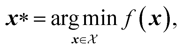
 is the optimization domain, or parameter space; i.e., the space of all experimental conditions that could have been explored during the optimization. In a Bayesian optimization setting, the objective function f is considered to be unknown, but can be empirically evaluated at specific values of x. Evaluating f(x) is assumed to be expensive and/or time consuming, and its measurement subject to noise. We also assume that we have no access to gradient information about f.
In a constrained optimization problem, one is interested in solutions within a subset of the optimization domain,  . This may be because f can be evaluated only for this subset, or because of user preference. In the QRAK taxonomy of Digabel and Wild,41 the former scenario would be that of known, nonquantifiable, unrelaxable, a priori constraints, or 4:NUAK constraints; the latter scenario would fall into the domain of relaxable constraints. In this work, we focus on unrelaxable constraints, even though the approach would be applicable also to the relaxable case.
A constraint function c(x) determines which parameters x are feasible and thus in  , and which are not. Contrary to unknown constraints, known constraints are those for which we have access to c(x) a priori, that is, we are aware of them before performing the optimization. Importantly, we can evaluate the functions c(x) and f(x) independently of one another. The solution of this constrained optimization problem may be written formally as
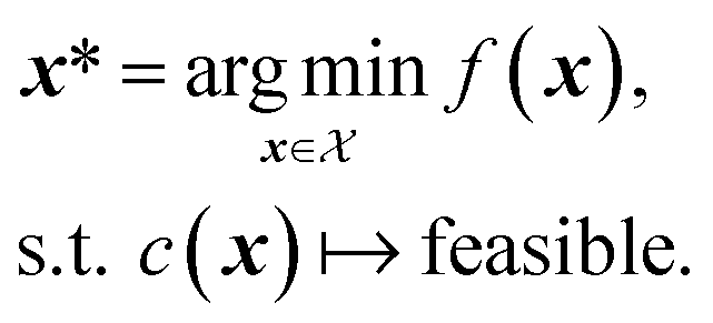
The physical meaning of c(x) is case dependent and domain specific. In chemistry, known constraints may reflect safety concerns, physical limits imposed by laboratory equipment, or simply researcher preference. The types of known constraints we focus on in this work are hard, unrelaxable constraints. They restrict  irrefutably and no measurement outside of
  is permitted. However, the use of soft constraints is also possible and has been explored. While soft constraints bias the optimization algorithm away from regions thought to yield undesirable outcomes, they ultimately still allow the full exploration of
  . In the relaxable scenario, imposing soft constraints can be a strategy to collect useful information outside of the desirable region
  . Soft constraints have also been used as means to introduce inductive biases into an optimization campaign based on prior knowledge.42,43
The goal of this work is to equip GRYFFIN with the ability to satisfy arbitrary constraints, as described by a user-defined constraint function c(x). This can be achieved by constraining the optimization of the acquisition function α.44α(x) defines the utility (or risk) of evaluating the parameters x, and the parameters proposed by the algorithm are those that optimize α(x). Thus, constrained optimization of the acquisition function also constrains the overall optimization problem accordingly. However, contrary to objective function f, the acquisition function α is easy to optimize, as its analytical form is known and can be evaluated cheaply. In the next sections we describe GRYFFIN's acquisition function and the approaches we implemented for its constrained optimization. Yet, note that any other constrained optimization algorithm handling nonlinear, nonconvex, and possibly discontinuous constraint functions could also be used.
A. Acquisition optimization in GRYFFIN
GRYFFIN's acquisition function, which is to be minimized, is defined as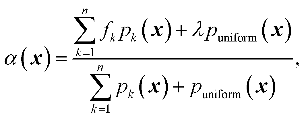 | (1) |
For continuous parameters, GRYFFIN uses Gaussian kernels with prior precision τ sampled from a Gamma distribution, τ ∼ Γ(a,b), with prior hyperparameters a = 12n2 and b = 1. For categorical and discrete parameters, it uses Gumbel-Softmax45,46 kernels with a prior temperature parameter of 0.5 + 10n−1. These prior parameters are, however, updated by a Bayesian neural network in light of the observed data.29 As the prior precision of the kernels increases with the number of observations, the surrogate model is encouraged to fit the observations more accurately as more data is acquired.
Acquisition function optimization in GRYFFIN generally follows a two-step strategy in which a global search is followed by local refinement. Effectively, it is a simple multi-start strategy that is memoryless and easily parallelizable. First, sets of input parameters xi are sampled uniformly from the optimization domain. By default, the number of samples is set to be directly proportional to the dimensionality of the optimization domain. Then, continuous parameters are optimized with a gradient method for a pre-defined number of iterations. While early versions of GRYFFIN employed second order methods such as L-BFGS, the default gradient-based approach is now Adam.47 Adam is a first-order, gradient-based optimization algorithm with momentum, which computes adaptive learning rates for each parameter by considering the first and second moments of the gradient. It thus naturally adjusts step size, and it is invariant to rescaling of gradients. Adam has found broad application for the optimization of neural network weights thanks to its robust performance. Categorical and discrete parameters are optimized instead following a hill-climbing approach (which we refer to as Hill), in which each initial sample xi is modified uniformly at random, one dimension at a time, and each move is accepted only if it improves α(xi).
In addition to gradient-based optimization of the acquisition function, in this work we have implemented gradient-free optimization via a genetic algorithm. The population of parameters is firstly selected uniformly at random, as described above. Then, each xi in the population is evolved via crossover, mutation and selection operations, with elitism applied. This approach handles continuous, discrete, and categorical parameters by applying different mutations and cross-over operations depending on the type. A more detailed explanation of the genetic algorithm used for acquisition optimization is provided in ESI Sec. S.1.B.† This approach is implemented in Python and makes use of the DEAP library.48,49
Fig. 1 provides a visual example of how these two approaches optimize the acquisition function of GRYFFIN. While Adam optimizes each random sample xi (black crosses) via small steps towards better α(xi) values (grey to white crosses), the genetic approach does so via larger stochastic jumps in parameter space.
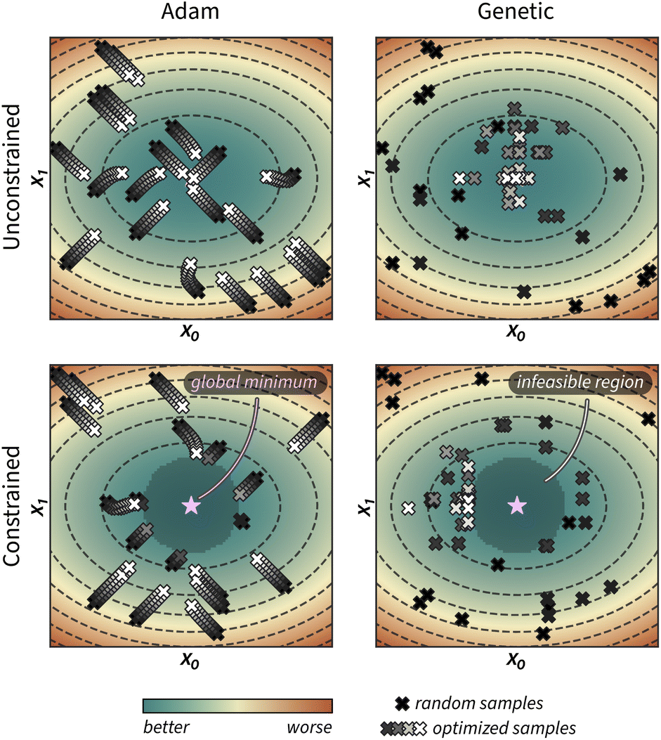 | ||
| Fig. 1 Illustration of unconstrained (top row) and constrained (bottom row) acquisition function optimization using strategies based on the Adam optimizer and a genetic algorithm. Initial, random samples are shown as black crosses. Grey crosses represent the updated parameter locations for these initial samples, while white crosses show the final locations after ten optimization iterations. The purple star indicates the global optima of the unconstrained acquisition function, which lies in the infeasible region in the constrained example. | ||
B. Constrained acquisition optimization with Adam or Hill
To constrain the optimization of the acquisition function according to a user-defined constraint function c(x), we first sample a set of feasible parameters xi with rejection sampling. That is, we sample uniformly from the optimization domain and we retain only samples that satisfy the constraint function c(x). Sampling is performed until the desired number of feasible samples is drawn. Local optimization of parameters is then performed with Adam, as described above, but it is terminated as soon as an update results in c(xi) ↦ infeasible (Fig. 1). For categorical and discrete parameters, Hill is used rather than Adam, but the constraint protocol is equivalent. In this case, after rejection sampling, any move in parameter space is accepted only if it improves α(xi) and subject to
  . Because of this early termination, each initial sample can be optimized locally for a different number of iterations. Strategies that do not terminate the optimization but adapt the update rule may preserve the number of allocated iterations across all initial samples.
C. Constrained acquisition optimization with a genetic algorithm
The population of the genetic optimization procedure is initialized with rejection sampling as described above for gradient approaches. However, to keep the optimized parameters within the feasible region, a subroutine is used to project infeasible offsprings onto the feasibility boundary using binary search (ESI Sec. S.1.B†). In addition to guaranteeing that the optimized parameters satisfy the constraint function, this approach also ensures sampling of parameters close to the feasibility boundary (Fig. 1 and ESI Fig. S1†).Despite having implemented constraints in GRYFFIN independently, when preparing this manuscript we realized that known constraints in DRAGONFLY50 have been implemented following a very similar strategy. However, rather than projecting infeasible offspring solution on the feasibility boundary, DRAGONFLY relies solely on rejection sampling.
A practical advantage of the genetic optimization strategy is its favourable computational scaling compared to its gradient-based counterpart. We conducted benchmarks in which the time needed by GRYFFIN to optimize the acquisition function was measured for different numbers of past observations and parameter space dimensions (ESI Sec. S.1.C†). In fact, acquisition optimization is the most costly task in most Bayesian optimization algorithms, including GRYFFIN. The genetic strategy provided a speedup of approximately 5× over Adam when the number of observations was varied, and of approximately 2.5× when the dimensionality of the optimization domain was varied. The better time complexity of the zeroth-order approach is primarily due to derivatives of α(x) not having to be computed. In fact, our Adam implementation currently computes derivatives numerically. Future work will focus on deriving the analytical gradients for GRYFFIN's acquisition function, or taking advantage of automatic differentiation schemes, such that this gap might reduce or disappear in future versions of the code.
D. User interface
With user-friendliness and flexibility in mind, we extended GRYFFIN's Python interface such that it can take a user-defined constraint function among its inputs. As an example, the following code snippet shows an instantiation of GRYFFIN where the sum of two volumes is constrained.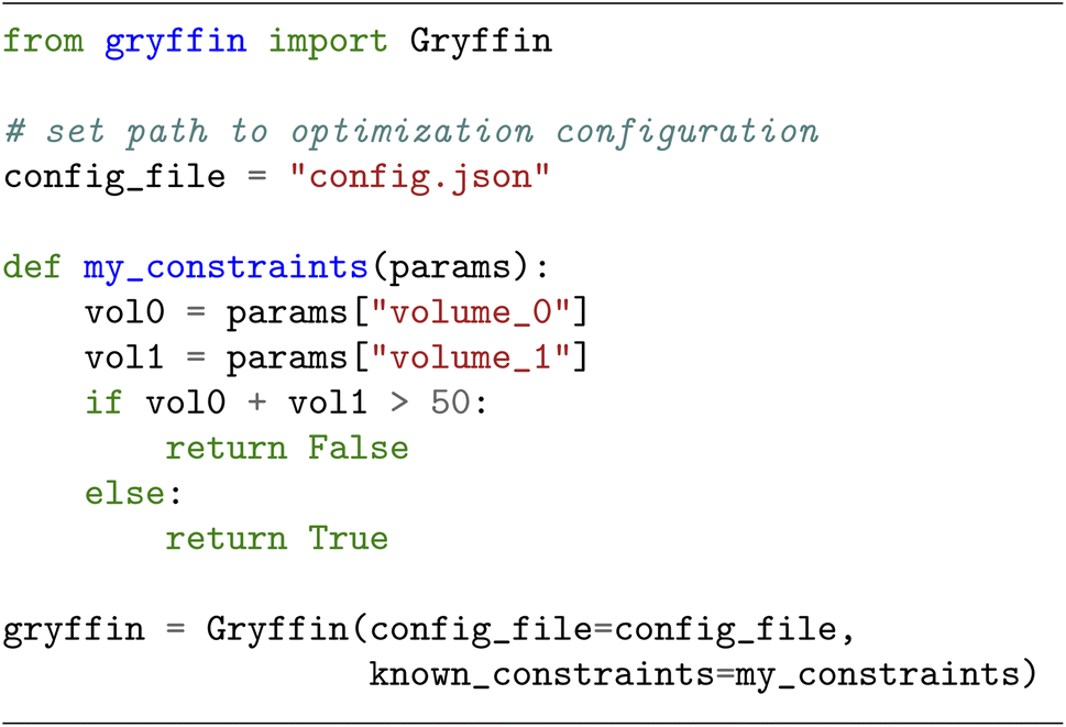
This example could be that of a minimization over two parameters, x = (x1,x2) ∈ [0,1]2, subject to the constraint that the sum of x1 and x2 does not exceed some upper bound b,
E. Current limitations
We note two limitations of our approach to known constraints. First, in continuous spaces, the current implementation handles only inequality constraints. Equality constraints, such as x1 + x2 = b, effectively change the dimensionality of the optimization problem and can be tackled via a re-definition of the optimization domain or analytical transforms. For instance, for the two-dimensional example above, the constraint can be satisfied simply by optimizing over x1, while setting x2 = b − x1.Second, because of the rejection sampling procedure used (Sec. II.B), the cost of acquisition optimization is inversely proportional to the fraction of the optimization domain that is feasible. The smaller the feasible volume fraction is, the more samples need to be drawn uniformly at random before reaching the predefined number of samples to be collected for acquisition optimization. It thus follows that the feasible region, as determined by the user-defined constraint function, should not be exceedingly small (e.g., less than 1% of the optimization domain), as in that case GRYFFIN's acquisition optimization would become inefficient. In practice we find that when only a tiny fraction of the overall optimization domain is considered feasible, it is because of a sub-optimal definition of the optimization domain, which can be solved by re-framing the problem. A related issue may arise if the constraints define disconnected feasible regions with vastly different volumes. In this scenario, given uniform sampling, little or no samples may be drawn from the smaller region. However, this too is an edge case that is unlikely to arise in practical applications, as the definition of completely separate optimization regions with vastly different scales tends to imply a scenario where multiple separate optimizations would be a more suitable solution.
Future work will focus on overcoming these two challenges. For instance, deep learning techniques like invertible neural networks51 may be used to learn a mapping from the unconstrained to the constrained domain, such that the optimization algorithm would be free to operate on the hypercube while the proposed experimental conditions would satisfy the constraints.
III. Results and discussion
In this section we test the ability of GRYFFIN to handle arbitrary known constraints. First, we show how GRYFFIN can efficiently optimize continuous and discrete (ordered) benchmark functions with a diverse set of constraints. Then, we demonstrate the practical utility of handling known constraints on two relevant chemistry examples: the optimization of the synthesis of o-xylenyl Buckminsterfullerene adducts under constrained flow conditions, and the design of redox active molecules for flow batteries under synthetic accessibility constraints.In addition to testing GRYFFIN—with both gradient and evolutionary based-acquisition optimization strategies, referred to as Gryffin (Adam/Hill) and Gryffin (Genetic), respectively—we also test three other constrained optimization strategies amenable to experiment planning. Specifically, we use random search (Random), a genetic algorithm (Genetic), and Bayesian optimization with a Gaussian process surrogate model (Dragonfly). Genetic is the same algorithm developed for constrained acquisition function optimization, but it is here employed directly to optimize the objective function (Sec. II.C). Dragonfly uses the DRAGONFLY package50 for optimization. Similar to GRYFFIN, DRAGONFLY allows for the specification of arbitrarily complex constraints via a Python function, which is not the case for most other Bayesian optimization packages. Dragonfly was not employed in the two chemistry examples, due to an implementation incompatibility with using both constraints and the multi-objective optimization strategy required by the applications.
A. Analytical benchmarks
Here, we use eight analytical functions (four continuous and four discrete) to test the ability of GRYFFIN to perform sample-efficient optimization while satisfying a diverse set of user-defined constraints. More specifically, we consider the following four two-dimensional continuous surfaces, as implemented in the OLYMPUS package:52Branin, Schwefel, Dejong, and Discrete Ackley (Fig. 2). While Branin has three degenerate global minima, we apply constraints such that only one minimum is present in the feasible region. In Schwefel, a highly unstructured constraint function is used, where the global minimum is close to the boundary of the infeasible region. In Dejong, we use a set of constraints that result in a non-compact optimization domain where the global minimum cannot be reached, and there is an infinite number of feasible minima along the feasibility boundary. Discrete Ackley is a discretized version of the Ackley function, and is an example of an extremely rugged surface. The four, two-dimensional discrete surfaces considered are: Slope, Sphere, Michalewicz, and Camel (Fig. 3). Each variable in these discrete surfaces is comprised of integer numbers from 0 to 20, for a design space of 441 options in total.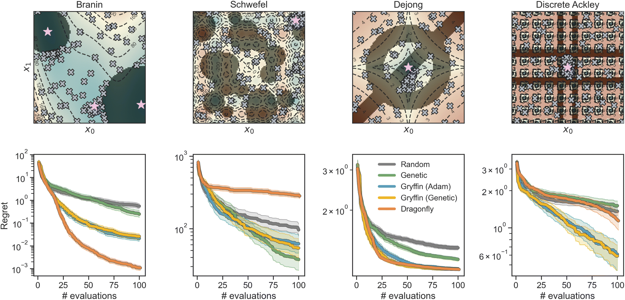 | ||
| Fig. 2 Constrained optimization benchmarks on analytical functions with continuous parameters. The upper row shows contour plots of the surfaces with constrained regions darkly shaded. Gray crosses show sample observation locations using the Gryffin (Genetic) strategy and purple stars denote the location(s) of unconstrained global optima. The bottom row show optimization traces for each strategy. Shaded regions around the solid trace represent 95% confidence intervals. | ||
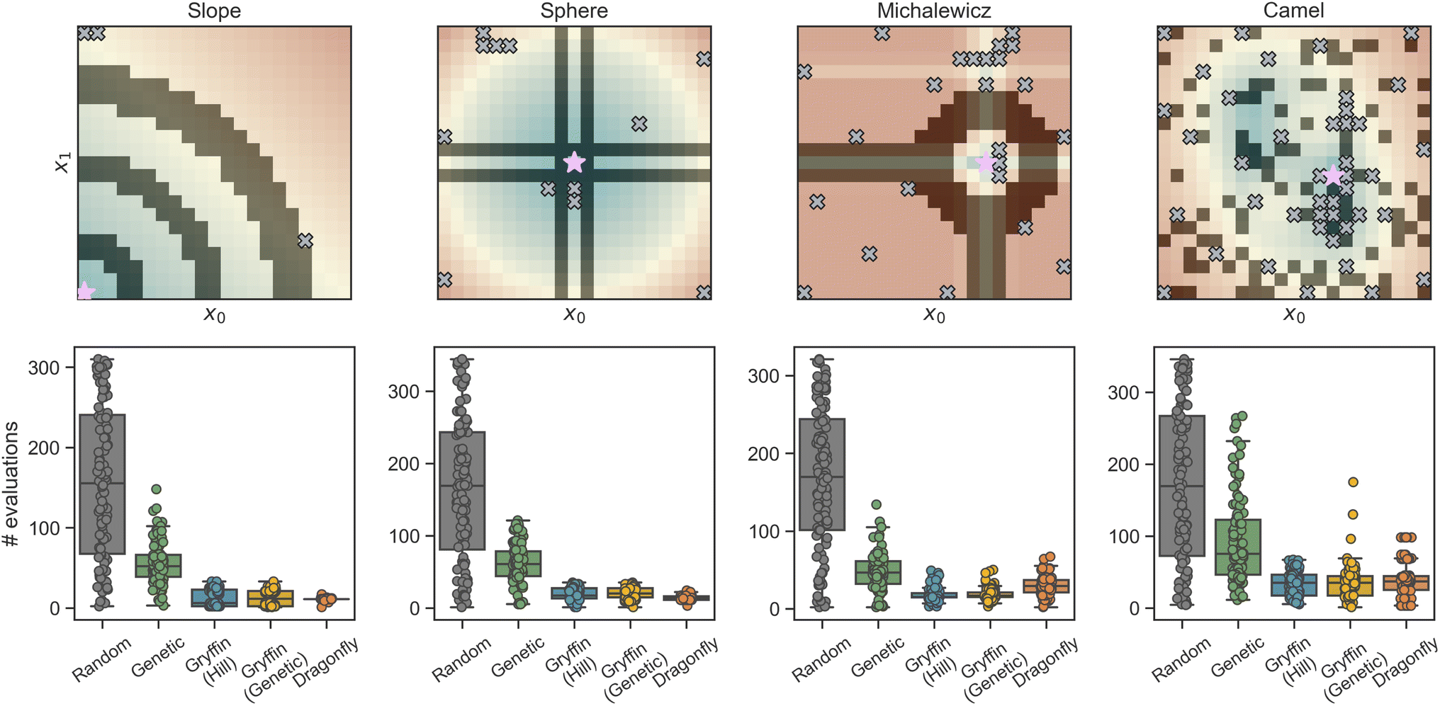 | ||
| Fig. 3 Constrained optimization benchmarks on analytical functions with discrete, ordered parameters. The upper row shows heatmaps of the discrete optimization domain. Shaded regions indicate infeasible regions, where constraints have been applied. The locations of the global optima are indicated by purple stars. Gray crosses show parameters locations that have been probed in a sample optimization run using Gryffin (Genetic) before the optimum being identified. The bottom row shows, as superimposed box-and-whisker and swarm plots, the distributions of the number of evaluations needed to identify the global optimum for each optimization strategy (numerical values can be found in Table S1†). | ||
Results of constrained optimization experiments on continuous surfaces are shown in Fig. 2. These results were obtained by performing 100 repeated optimizations for each of the five strategies considered, while allowing a maximum of 100 objective function evaluations. Optimization performance is assessed using the distance between the best function value found at each iteration of the optimization campaign and the global optimum, a metric known as regret, r. The regret after k optimization iterations is
| rk = |f(x*) − f(x+k)|. | (2) |
 , where
  is the current dataset of observations. x* are the parameters associated with the global optimum of the function within the whole optimization domain. If the optimum lies in the infeasible region, a regret of zero is not attainable. Sample-efficient algorithms should find parameters that return better (in this case lower) function values with fewer objective evaluations.
All optimization strategies tested obeyed the known constraints (Fig. 2, top row). We observe that the combination of analytical function and user-defined constraint have great influence on the relative optimization performance of the considered strategies. On all functions, the performance of GRYFFIN was insensitive to the acquisition optimization strategy, with Gryffin (Adam) and Gryffin (Genetic) performing equally well. This observation also held true on higher-dimensional surfaces (ESI Fig. S4†). On smooth functions, such as Branin and Dejong, Dragonfly displayed strong performance, given that its Gaussian process surrogate model approximates these functions extremely well. In addition, DRAGONFLY appears to propose parameter points that are closer to previous observations than GRYFFIN does, showcasing a more exploitative character, which in this case is beneficial to achieve marginal gains in performance when in very close proximity to the optimum (see ESI Sec. S.2.C for additional details†). Although their performance is slightly worse than Dragonfly, Gryffin strategies still displayed improved performance over Random and Genetic on Branin, and comparable performance to Dragonfly on Dejong. Gryffin strategies showed improved performance compared to Dragonfly on Schwefel and Discrete Ackley. These observations are consistent with previous work29 where it was observed that, due to the different surrogate models used, GRYFFIN returned better performance on functions with discontinuous character, while Gaussian process-based approaches better performed on smooth surfaces. On Schwefel, our Genetic strategy also showed improved performance over that of Random and Dragonfly, comparable with that of Gryffin. It is interesting to note how Dragonfly performed particularly poorly on this function. This is due to Schwefel being a periodic function, while the prior used by Dragonfly is the Matérn kernel. When using a periodic kernel with suitable inductive biases, the Gaussian process model better fits the surface, locating the global minimum (ESI Fig. S5†). Finally, note that in Fig. 2 differences between strategies are exaggerated by the use of a logarithmic scale, used to highlight statistically significant differences. We also report the same results using a linear scale, which de-emphasizes significant yet marginal differences in regret values (e.g. between Dragonfly and Gryffin on the Branin function) in ESI Fig. S3.†
Results of constrained optimization experiments on discrete synthetic surfaces are shown in Fig. 3. These results are also based on 100 repeated optimizations, each initialized with a different random seed. Optimizations were allowed to continue until the global optimum was found. As a measure of performance, the number of objective function evaluations required to identify the optimum was used. As such, a more efficient algorithm should identify the optimum with fewer evaluations on average.
Here too, all strategies tested correctly obeyed each constraint function (Fig. 3, top row), and Bayesian optimization algorithms (Gryffin and Dragonfly) outperformed Random and Genetic on all four benchmarks (Fig. 3, bottom row). Random needed to evaluate about half of the feasible space before identifying the optimum. Genetic required significantly fewer evaluations, generally between a half and a third of those required by Random. On discrete surfaces, the approaches based on GRYFFIN and DRAGONFLY returned equal performance overall, with no considerable differences (Table S1†). As it was observed for continuous surfaces, the performance of Gryffin (Adam) and Gryffin (Genetic) was equivalent.
In settings where the constraints are the result of limitations in experimental capabilities, one may want to evaluate whether the global optimum could be located in the infeasible region, with the goal of deciding whether to expand such capabilities. While this task is best suited to a supervised learning framework, in which multiple ML models could be evaluated for their predictive ability, the data collected by the optimization algorithm is what enables such models. It is therefore interesting to notice how GRYFFIN tends to collect data that is likely informative for this task. In fact, the combination of GRYFFIN's acquisition function and its constrained optimization results in a data-collection strategy that tends to probe the boundaries of the feasibility region, with a higher density of points in proximity of possible minima. Examples of this behavior may be seen in Fig. 2 for the Branin and Dejong functions, which have their global optima located in the infeasible (constrained) region. In these cases, GRYFFIN sampled a higher density of points on the feasibility boundary close to these optima. These data points would be useful when building a ML model that tries to extrapolate into the infeasible region.
B. Process-constrained optimization of o-xylenyl C60 adducts synthesis
Compared to their inorganic counterparts, organic solar cells have the advantage of being flexible, lightweight and easily fabricated.53,54 Bulk heterojunction polymer-fullerene cells are an example of such devices, in which the photoactive layer is composed of a blend of polymeric donor material and fullerene derivative acceptor molecules.55 The fullerene acceptor is oftentimes functionalized to tune its optoelectronic properties. In particular, mono and bis o-xylenyl adducts of Buckminsterfullerene are acceptor molecules which have received much attention in this regard. On the other hand, higher-order adducts are avoided as they have a detrimental impact on the power conversion efficiencies of the resulting device.56 Therefore, synthetic protocols that provide accurate control over the degree of C60 functionalization are of primary interests for the manufacturing of these organic photovoltaic devices.In this example application of constrained Bayesian optimization, we consider the reaction of C60 with an excess of sultine, the cyclic ester of a hydroxy sulfinic acid, to form first, second, and third order o-xylenyl adducts of Buckminsterfullerene (Fig. 4a). This application is based on previous work by Walker et al.,35 who reported the optimization of this reaction with an automated, single-phase capillary-based flow reactor. Because this reaction is cascadic, a mixture of products is always present, with the relative amounts of each species depending primarily on reaction kinetics. The overall goal of the optimization is thus to tune reaction conditions such that the yield of first- and second-order adducts is maximized and reaches at least 90%, while the cost of reagents is minimized. We estimated reagents cost by considering the retail price listed by a chemical supplier (ESI Sec. S.3.B†). In effect, we derive a simple estimate of per-minute operation cost of the flow reactor, which is to be minimized as the second optimization objective.
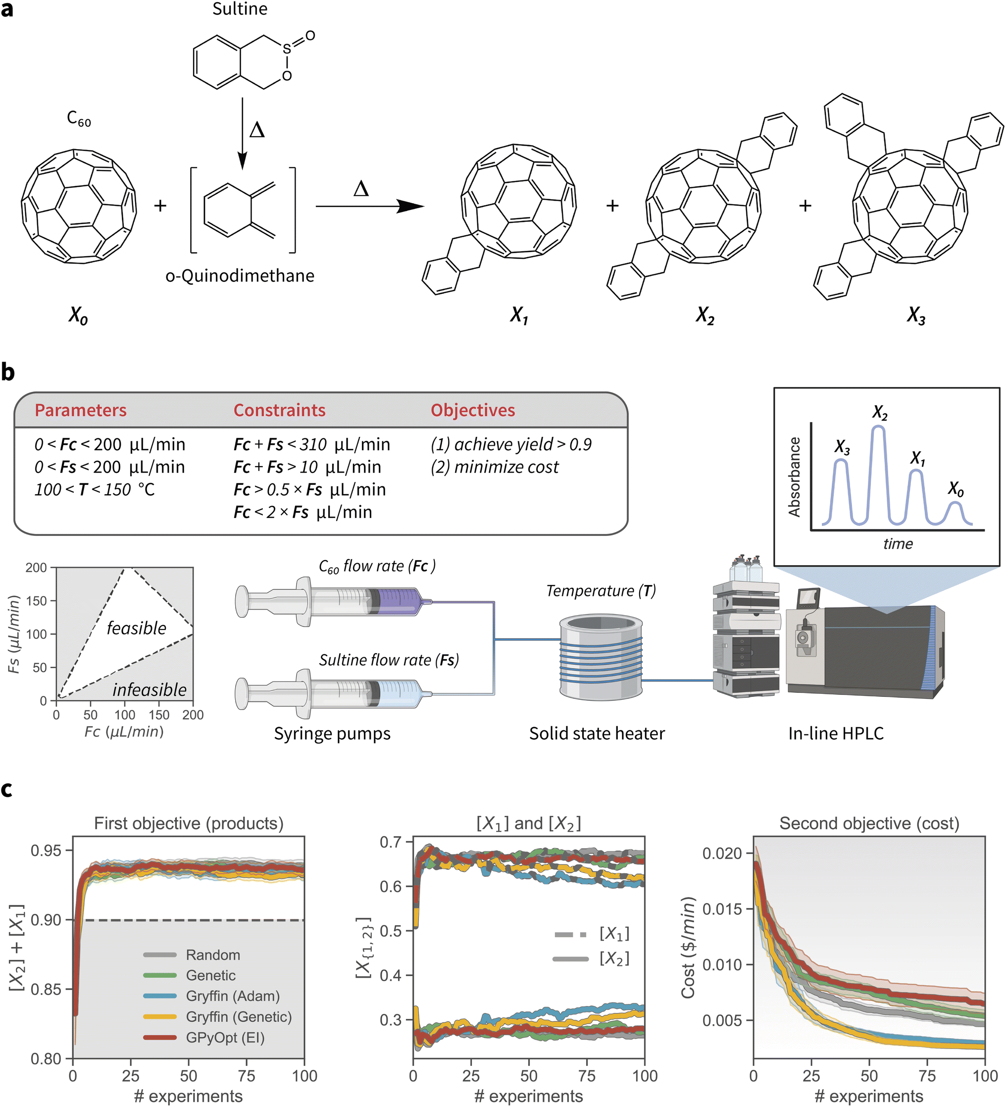 | ||
| Fig. 4 Experimental setup and results of the process-constrained synthesis of o-xylenyl C60 adducts. (a) Synthesis of o-xylenyl C60 adducts. 1,4-dihydro-2,3-benzoxathiin 3-oxide (sultine) is converted to o-quinidimethane (oQDM) in situ, which then reacts with C60 by Diels–Alder cycloaddition to form the o-xylenyl adducts. (b) Schematic of the single-phase capillary-based flow reactor (as reported by Walker et al.35), along with the optimization parameters, constraints, and objectives. The C60 and sultine flow rates are modulated by syringe pumps, and the reaction temperature is controlled by a solid state heater. Online HPLC and absorption spectroscopy is used for analysis. (c) Results of the constrained optimization experiments. Plots show the mean and 95% confidence interval of the best objective values found after varying numbers of experiments, for each optimization algorithm studied. The background color indicates the desirability of the objective values, with grey being less, and white more desirable. For the first objective (left-hand side), the grey region below the value of 0.9 indicates values for the objective that do not satisfy the optimization goal that was set. | ||
The controllable reaction conditions are the temperature (T), the flow rate of C60 (FC), and the flow rate of sultine (FS), which determine the chemical composition of the reaction mixture and are regulated by syringe pumps (Fig. 4b). T is allowed to be set anywhere between 100 and 150 °C, and flow rates can be varied between 0 and 200 μL min−1. However, the values of the flow rates are constrained. First, the total flow rate cannot exceed 310 μL min−1, or be below 10 μL min−1. Second, FS cannot be more than twice FC, and vice versa FC cannot be more than twice FS. More formally, the inequality constraints can be defined as 10 < FC + FS < 310 μL min−1, FC < 2FS and FS < 2FC.
The relative concentrations of each adduct—[X1], [X2], and [X3] for the mono, bis, and tris adduct, respectively—are measured via online high-performance liquid chromatography (HPLC) and absorption spectroscopy. Following from the above discussion, we would like to maximize the yield of [X1] and [X2], which are the adducts with desirable optoelectronic properties. However, we would also like to reduce the overall cost of the raw materials. These multiple goals are captured via the use of CHIMERA as a hierarchical scalarizing function for multi-objective optimization.31 Specifically, we set the first objective as the maximization of [X1] + [X2], with a minimum target goal of 0.9, and the minimization of reagents cost as the secondary goal. Effectively, this setup corresponds to the minimization of cost under the constraint that [X1] + [X2] ≥ 0.9.
To perform numerous repeated optimizations with different algorithms, as well as collect associated statistics, we constructed a deep learning model to simulate the above-described experiment. In particular, we trained a Bayesian neural network based on the data provided by Walker et al.,35 which learns to map reaction conditions to a distribution of experimental outcomes (ESI Sec. S.3.A†). The measurement is thus stochastic, as expected experimentally. This emulator takes T, FC, and FS as input, and returns mole fractions of the un- (X0), singly- (X1), doubly- (X2), and triply-functionalized (X3) C60. The model displayed excellent interpolation performance across the parameter space for each adduct type (Pearson coefficient of 0.93–0.96 on the test sets). This enabled us to perform many repeated optimizations thanks to rapid and accurate simulated experiments.
Results of the constrained optimization experiments are shown in Fig. 4c. Optimization traces show the objective values associated with the best scalarized merit value. The constrained GRYFFIN strategies obeyed all flow rate constraints defined. All strategies rapidly identified reaction conditions producing high yields. Upon satisfying the first objective, CHIMERA guided the optimization algorithms towards lowering the cost of the reaction. GRYFFIN achieved cheaper protocols faster than the other strategies tested. In ESI Sec. S.3.B† we examine the best reactions conditions identified by each optimization strategy after 100 experiments. We find that for the majority of cases, strategies decreased the C60 flow rate (the more expensive reagent) to minimize the cost of the experiment, while simultaneously decreasing the sultine flow rate to maintain a stoichiometric ratio close to one and preserve the high (≥0.9 combined mole fraction) yield of X0 and X1 adducts. In principle, the yield is allowed to degrade with an accompanying decrease (improvement) in cost. However, we did not see the trade-off between yield and cost being required within the experimental budget of 100 experiments. In this case study we used GPYOPT, as opposed to DRAGONFLY, as a representative of an established Bayesian optimization algorithm, because its implementation was compatible with the requirements of this specific scenario. That is, the presence of known constraints and the use of an external scalarizing function for multi-objective optimization. Use of CHIMERA as an external scalarizing function requires updating the entire optimization history at each iteration. Thus, the optimization library must be used via an ask-tell interface. Although DRAGONFLY does have such an interface, to the best of our knowledge it does not yet support constrained and multi-objective optimizations with external scalarizing functions. In this instance, GPYOPT with expected improvement as the acquisition function performed similarly to Genetic and Random on average.
As a final note, we point out that in this application the reaction conditions were assumed to be constant throughout each experiment. However, other setups may involve time-varying parameters. When this is done in a controlled fashion, additional parameters can be used to describe a time-dependent protocol. For instance, a linear temperature gradient can be described by three variables: initial temperature, a time interval, and the rate of temperature change over time. If changes in the controllable parameters are undesirable consequences of shortcomings of the protocol or equipment (e.g., limited temperature control ability), these may be accounted for by considering the input parameter as uncertain.32
C. Design of redox-active materials for flow batteries with synthetic accessibility constraints
Long-duration, stationary energy storage devices are needed to handle the rapid growth in intermittent energy sources.58 Toward this goal, redox flow batteries offer a potentially promising solution.59–63 Second-generation non-aqueous redox flow batteries are based on organic solvent as opposed to water, which enables a much larger electrochemical window and higher energy density, the potential to increase the working temperature window, as well as the use of cheap, earth abundant redox-active materials.64 Nevertheless, the multiobjective design of redox-active materials poses a significant challenge in materials science. Recently, the anolyte redox material 2,1,3-benzothiadiazole was shown to have low redox potential, high stability and promising electrochemical cycling performance.65–67 Furthermore, derivatization of benzothiadiazole enabled self-reporting of battery health by fluorescence emission.68In this application we demonstrate our constrained optimization approach for the multi-objective design of retro-synthetically accessible redoxmer molecules. We utilize a previously reported dataset that comprises 1408 benzothiadiazole derivatives (Fig. 5a) for which the reduction potential Ered, solvation free energy Gsolv, and maximum absorption wavelength λabs were computed with DFT.69 This example application thus simulates a DFT-based computational screen70–72 that aims to identify redoxmer candidates with self-reporting features and a high probability of synthetic accessibility.
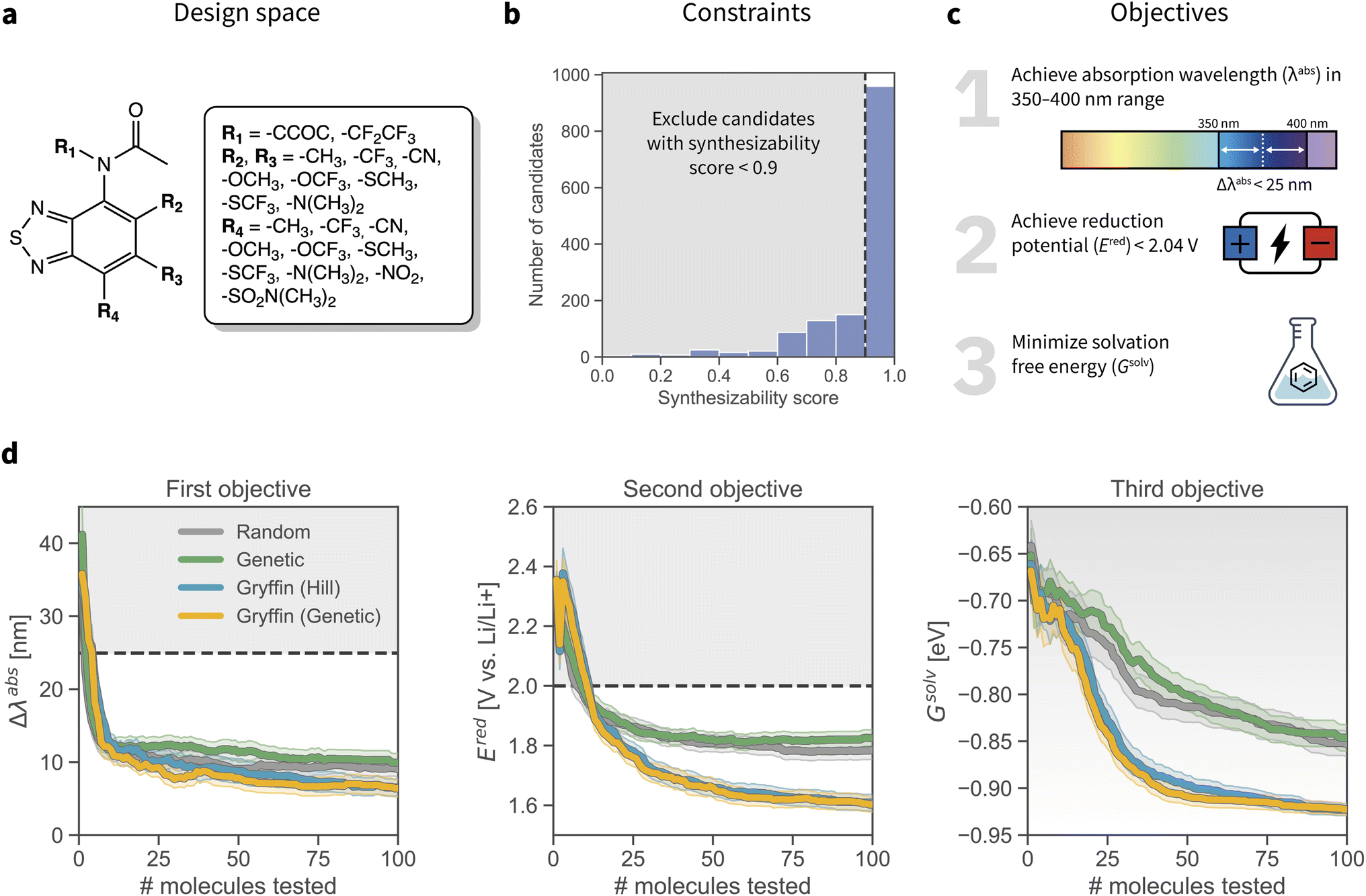 | ||
| Fig. 5 Optimization setup and results for the design of redox-active materials. (a) Markush structure of the benzothiadiazole scaffold and all substituents considered. The entire design space consists of 1408 candidates (2 R1 × 8 R2 × 8 R3 × 11 R4 options). (b) Synthetic constraints applied to the optimization. The RAscore57 was used to score synthesizability. The histogram shows the distribution of synthesizability scores for all 1408 candidates. We constrain the optimization to those candidates with an RAscore > 0.9. (c) Objectives of the molecular optimization. (d) Results of the constrained optimization experiments. Grey shaded regions indicate objective values failing to achieve the desired objectives. Traces depict the objective values corresponding to the best achieved merit at each iteration, where error bars represent 95% confidence intervals. | ||
To impose synthetic accessibility constraints we used RAscore,57 a recently-reported synthetic accessibility score based on the computer-aided synthesis planner AiZythFinder.73RAscore predicts the probability of AiZythFinder being able to identify a synthetic route for a target organic molecule. While other measures of synthetic accessibility are available,34,74–76RAscore was chosen for its performance and intuitive interpretation. In our experiments, we constrained the optimization to candidates with RAscore > 0.9 (Fig. 5b, additional details in ESI Sec. S.4.B†). This synthetic accessibility constraint reduces the design space of feasible candidates to a total of 959 molecules.
We aimed at optimizing three objectives concurrently: the absorption wavelength λabs, the reduction potential Ered, and the solvation free energy Gsolv of the candidates (Fig. 5c). Specifically, we aimed at identifying molecules that would (i) absorb in the 350–400 nm range, (ii) improve upon the reduction potential of the base scaffold (2.04 V against a Li/Li+ reference electrode; ESI Sec. S.4.A†), and (iii) provide the lowest possible solvation free energy, here used as a proxy for solubility. The hierarchical scalarizing function CHIMERA31 was used to guide the optimization algorithms toward achieving these desired properties.
Results of the constrained optimization experiments are displayed in Fig. 5d. Each optimization strategy was given a budget of 100 molecules to be tested; the experiments were repeated 100 times and initialized with different random seeds. Optimization traces show the values of Δλabs, Ered, and Gsolv associated with the best molecule identified among those tested. In these tests, the dynamic version of GRYFFIN was used.30 This approach can take advantage of physicochemical descriptors in the search for optimal molecules. In this case, GRYFFIN was provided with several descriptors for each R group in the molecule: number of heavy atoms, number of hetero atoms, molecular weight, geometric diameter, polar surface area, polarizability, fraction of sp3 carbons (ESI Sec. S.4.C†).77
Constrained GRYFFIN avoided redoxmer candidates predicted to be retro-synthetically inaccessible. All optimization strategies rapidly identified candidates with λabs between 350 and 400 nm, and whose Ered is lower than that of the starting scaffold. However, GRYFFIN strategies managed to identify candidates with lower Gsolv faster than Random and Genetic. Consistent with previous tests, we did not observe a statistically different performance between Gryffin (Hill) and Gryffin (Genetic). Overall, Gryffin (Hill) and Gryffin (Genetic) identified molecules with better λabs, Ered, and Gsolv properties than Random or Genetic after probing 100 molecules. Furthermore, within this budget, GRYFFIN identified molecules with better properties more efficiently than the competing strategies tested. Without the aid of physicochemical descriptors, GRYFFIN's performance deteriorated, as expected,30 yet it was still superior than that of Random and Genetic (ESI Fig. S11†).
IV. Conclusion
In this work, we extended the capabilities of GRYFFIN to handle a priori known, hard constraints on the parameter domain, a pragmatic requirement for the development of autonomous research platforms in chemistry. Known constraints constitute an important class of restrictions placed on optimization domains, and may reflect physical constraints or limitations in laboratory equipment capabilities. In addition, known constraints may provide a straightforward avenue to inject prior knowledge or intuition into a chemistry optimization task.In GRYFFIN, we allow the user to define arbitrary known constraints via a flexible and intuitive Python interface. The constraints are then satisfied by constraining the optimization of its acquisition function.
In all our benchmarks, GRYFFIN obeyed the (sometimes complex) constraints defined, showed superior performance to more traditional search strategies based on random search and evolutionary algorithms, and was competitive to state-of-the-art Bayesian optimization approaches.
Finally, we demonstrated the practical utility of handling known constraints with GRYFFIN in two research scenarios relevant to chemistry. In the first, we demonstrated how to perform an efficient optimization for the synthesis of o-xylenyl adducts of Buckminsterfullerene while subjecting the experimental protocol to process constraints. In the second, we showed how known constraints may be used to incorporate synthetic accessibility considerations in the design of redox active materials for non-aqueous flow batteries.
It is our hope that simple, flexible, and scalable software tools for model-based optimization over constrained parameter spaces will enhance the applicability of data-driven optimization in chemistry and material science, and will contribute to the operationalization of self-driving laboratories.
Data availability
An open-source implementation of GRYFFIN with known constraints is available on GitHub at https://github.com/aspuru-guzik-group/gryffin, under an Apache 2.0 license. The data and scripts used to run the experiments and produce the plots in this paper are also available on GitHub at https://github.com/aspuru-guzik-group/gryffin-known-constraints.Conflicts of interest
A. A.-G. is the Chief Visionary Officer and founding member of Kebotix, Inc.Acknowledgements
The authors thank Dr Martin Seifrid, Marta Skreta, Ben Macleod, Fraser Parlane, and Michael Elliott for valuable discussions. R. J. H. gratefully acknowledges the Natural Sciences and Engineering Research Council of Canada (NSERC) for provision of the Postgraduate Scholarships-Doctoral Program (PGSD3-534584-2019). M. A. was supported by a Postdoctoral Fellowship of the Vector Institute. A. A.-G. acknowledges support from the Canada 150 Research Chairs program and CIFAR, as well as the generous support of Anders G. Fröseth. This work relates to the Department of Navy award (N00014-18-S-B-001) issued by the office of Naval Research. The United States Government has a royalty-free license throughout the world in all copyrightable material contained herein. Any opinions, findings, and conclusions or recommendations expressed in this material are those of the authors and do not necessarily reflect the views of the Office of Naval Research. Computations reported in this work were performed on the computing clusters of the Vector Institute and on the Niagara supercomputer at the SciNet HPC Consortium.78,79 Resources used in preparing this research were provided, in part, by the Province of Ontario, the Government of Canada through CIFAR, and companies sponsoring the Vector Institute. SciNet is funded by the Canada Foundation for Innovation, the Government of Ontario, Ontario Research Fund – Research Excellence, and by the University of Toronto.References
- A. McNally, C. K. Prier and D. W. C. MacMillan, Science, 2011, 334(6059), 1114–1117 CrossRef CAS PubMed.
- K. D. Collins, T. Gensch and F. Glorius, Nat. Chem., 2014, 6, 859–871 CrossRef CAS PubMed.
- V. Blay, B. Tolani, S. P. Ho and M. R. Arkin, Drug Discovery Today, 2020, 25, 1807–1821 CrossRef CAS.
- W. Zeng, L. Guo, S. Xu, J. Chen and J. Zhou, Trends Biotechnol., 2020, 38, 888–906 CrossRef CAS.
- L. Cheng, R. S. Assary, X. Qu, A. Jain, S. P. Ong, N. N. Rajput, K. Persson and L. A. Curtiss, J. Phys. Chem. Lett., 2015, 6, 283–291 CrossRef CAS PubMed.
- J. Močkus, Optimization techniques IFIP technical conference, 1975, pp. 400–404 Search PubMed.
- J. Mockus, V. Tiesis and A. Zilinskas, Towards Global Optimization, 1978, vol. 2, p. 2 Search PubMed.
- J. Mockus, Bayesian approach to global optimization: theory and applications, Springer Science & Business Media, 2012, vol. 37 Search PubMed.
- B. J. Shields, J. Stevens, J. Li, M. Parasram, F. Damani, J. I. M. Alvarado, J. M. Janey, R. P. Adams and A. G. Doyle, Nature, 2021, 590, 89–96 CrossRef CAS.
- M. Christensen, L. P. E. Yunker, F. Adedeji, F. Häse, L. M. Roch, T. Gensch, G. dos Passos Gomes, T. Zepel, M. S. Sigman, A. Aspuru-Guzik and J. E. Hein, Commun. Chem., 2021, 4(1), 112 CrossRef.
- M. Reis, F. Gusev, N. G. Taylor, S. H. Chung, M. D. Verber, Y. Z. Lee, O. Isayev and F. A. Leibfarth, J. Am. Chem. Soc., 2021, 143, 17677–17689 CrossRef CAS PubMed.
- S. Langner, F. Häse, J. D. Perea, T. Stubhan, J. Hauch, L. M. Roch, T. Heumueller, A. Aspuru-Guzik and C. J. Brabec, Adv. Mater., 2020, 32, 1907801 CrossRef CAS.
- B. P. MacLeod, F. G. L. Parlane, T. D. Morrissey, F. Häse, L. M. Roch, K. E. Dettelbach, R. Moreira, L. P. E. Yunker, M. B. Rooney, J. R. Deeth, V. Lai, G. J. Ng, H. Situ, R. H. Zhang, M. S. Elliott, T. H. Haley, D. J. Dvorak, A. Aspuru-Guzik, J. E. Hein and C. P. Berlinguette, Sci. Adv., 2020, 6, eaaz8867 CrossRef CAS.
- D. E. Graff, E. I. Shakhnovich and C. W. Coley, Chem. Sci., 2021, 12, 7866–7881 RSC.
- A. E. Gongora, B. Xu, W. Perry, C. Okoye, P. Riley, K. G. Reyes, E. F. Morgan and K. A. Brown, Sci. Adv., 2020, 6, eaaz1708 CrossRef PubMed.
- F. Häse, L. M. Roch and A. Aspuru-Guzik, Trends Chem., 2019, 1, 282–291 CrossRef.
- L. M. Roch, F. Häse, C. Kreisbeck, T. Tamayo-Mendoza, L. P. E. Yunker, J. E. Hein and A. Aspuru-Guzik, PLoS One, 2020, 15, e0229862 CrossRef CAS PubMed.
- J.-P. Correa-Baena, K. Hippalgaonkar, J. van Duren, S. Jaffer, V. R. Chandrasekhar, V. Stevanovic, C. Wadia, S. Guha and T. Buonassisi, Joule, 2018, 2, 1410–1420 CrossRef CAS.
- H. S. Stein and J. M. Gregoire, Chem. Sci., 2019, 10, 9640–9649 RSC.
- E. Stach, B. DeCost, A. G. Kusne, J. Hattrick-Simpers, K. A. Brown, K. G. Reyes, J. Schrier, S. Billinge, T. Buonassisi, I. Foster, C. P. Gomes, J. M. Gregoire, A. Mehta, J. Montoya, E. Olivetti, C. Park, E. Rotenberg, S. K. Saikin, S. Smullin, V. Stanev and B. Maruyama, Matter, 2021, 4, 2702–2726 CrossRef.
- C. W. Coley, N. S. Eyke and K. F. Jensen, Angew. Chem., Int. Ed., 2020, 59, 22858–22893 CrossRef CAS PubMed.
- C. W. Coley, N. S. Eyke and K. F. Jensen, Angew. Chem., Int. Ed., 2020, 59, 23414–23436 CrossRef CAS PubMed.
- B. Burger, P. M. Maffettone, V. V. Gusev, C. M. Aitchison, Y. Bai, X. Wang, X. Li, B. M. Alston, B. Li, R. Clowes, N. Rankin, B. Harris, R. S. Sprick and A. I. Cooper, Nature, 2020, 583, 237–241 CrossRef CAS PubMed.
- A. Dave, J. Mitchell, K. Kandasamy, H. Wang, S. Burke, B. Paria, B. Póczos, J. Whitacre and V. Viswanathan, Cell Rep. Phys. Sci., 2020, 1, 100264 CrossRef CAS.
- A. Deshwal, C. M. Simon and J. Rao Doppa, Mol. Syst. Des. Eng., 2021, 6, 1066–1086 RSC.
- A. G. Kusne, H. Yu, C. Wu, H. Zhang, J. Hattrick-Simpers, B. DeCost, S. Sarker, C. Oses, C. Toher, S. Curtarolo, A. V. Davydov, R. Agarwal, L. A. Bendersky, M. Li, A. Mehta and I. Takeuchi, Nat. Commun., 2020, 11, 5966 CrossRef CAS.
- H. Tao, T. Wu, S. Kheiri, M. Aldeghi, A. Aspuru-Guzik and E. Kumacheva, Adv. Funct. Mater., 2021, 31, 2106725 CrossRef CAS.
- P. B. Wigley, P. J. Everitt, A. van den Hengel, J. W. Bastian, M. A. Sooriyabandara, G. D. McDonald, K. S. Hardman, C. D. Quinlivan, P. Manju, C. C. N. Kuhn, I. R. Petersen, A. N. Luiten, J. J. Hope, N. P. Robins and M. R. Hush, Sci. Rep., 2016, 6, 25890 CrossRef CAS PubMed.
- F. Häse, L. M. Roch, C. Kreisbeck and A. Aspuru-Guzik, ACS Cent. Sci., 2018, 4, 1134–1145 CrossRef.
- F. Häse, M. Aldeghi, R. J. Hickman, L. M. Roch and A. Aspuru-Guzik, Appl. Phys. Rev., 2021, 8, 031406 Search PubMed.
- F. Häse, L. M. Roch and A. Aspuru-Guzik, Chem. Sci., 2018, 9, 7642–7655 RSC.
- M. Aldeghi, F. Häse, R. J. Hickman, I. Tamblyn and A. Aspuru-Guzik, Chem. Sci., 2021, 12, 14792–14807 RSC.
- R. J. Hickman, F. Häse, L. M. Roch and A. Aspuru-Guzik, 2021, arXiv, 2103.03391.
- M. Seifrid, R. J. Hickman, A. Aguilar-Granda, C. Lavigne, J. Vestfrid, T. C. Wu, T. Gaudin, E. J. Hopkins and A. Aspuru-Guzik, ACS Cent. Sci., 2022, 8, 122–131 CrossRef CAS PubMed.
- B. E. Walker, J. H. Bannock, A. M. Nightingale and J. C. deMello, React. Chem. Eng., 2017, 2, 785–798 RSC.
- M. A. Gelbart, J. Snoek and R. P. Adams, Proceedings of the Thirtieth Conference on Uncertainty in Artificial Intelligence, Arlington, Virginia, USA, 2014, pp. 250–259 Search PubMed.
- R. B. Gramacy and H. K. H. Lee, 2010, arXiv:1004.4027 [stat].
- M. A. Gelbart, J. Snoek and R. P. Adams, 2014, arXiv:1403.5607 [cs, stat].
- S. Ariafar, J. Coll-Font, D. Brooks and J. Dy, J. Mach. Learn. Res., 2019, 20, 1–26 Search PubMed.
- C. Antonio, J. Glob. Optim., 2021, 79, 281–303 CrossRef.
- S. L. Digabel and S. M. Wild, 2015, arXiv, 1505.07881.
- S. Sun, A. Tiihonen, F. Oviedo, Z. Liu, J. Thapa, Y. Zhao, N. T. P. Hartono, A. Goyal, T. Heumueller, C. Batali, A. Encinas, J. J. Yoo, R. Li, Z. Ren, I. M. Peters, C. J. Brabec, M. G. Bawendi, V. Stevanovic, J. Fisher III and T. Buonassisi, Matter, 2021, 4, 1305–1322 CrossRef CAS.
- Z. Liu, N. Rolston, A. C. Flick, T. Colburn, Z. Ren, R. H. Dauskardt and T. Buonassisi, 2021, arXiv:2110.01387 [physics].
- B. Shahriari, K. Swersky, Z. Wang, R. P. Adams and N. de Freitas, Proc. IEEE, 2016, 104, 148–175 Search PubMed.
- E. Jang, S. Gu and B. Poole, 5th International Conference on Learning Representations, ICLR 2017, Toulon, France, April 24–26, 2017, Conference Track Proceedings, 2017 Search PubMed.
- Y. W. T. Chris J. Maddison and A. Mnih, 5th International Conference on Learning Representations, ICLR 2017, Toulon, France, April 24–26, 2017, Conference Track Proceedings, 2017 Search PubMed.
- D. P. Kingma and J. Ba, arXiv:1412.6980 [cs], 2017.
- F.-A. Fortin, F.-M. De Rainville, M.-A. Gardner, M. Parizeau and C. Gagné, J. Mach. Learn. Res., 2012, 13, 2171–2175 Search PubMed.
- F.-M. De Rainville, F.-A. Fortin, M.-A. Gardner, M. Parizeau and C. Gagné, Proceedings of the 14th annual conference companion on Genetic and evolutionary computation, 2012, pp. 85–92 Search PubMed.
- K. Kandasamy, K. R. Vysyaraju, W. Neiswanger, B. Paria, C. R. Collins, J. Schneider, B. Poczos and E. P. Xing, J. Mach. Learn. Res., 2020, 21, 1–27 Search PubMed.
- J. Behrmann, W. Grathwohl, R. T. Q. Chen, D. Duvenaud and J.-H. Jacobsen, Proceedings of the 36th International Conference on Machine Learning, Long Beach, California, USA, 2019, pp. 573–582 Search PubMed.
- F. Häse, M. Aldeghi, R. J. Hickman, L. M. Roch, M. Christensen, E. Liles, J. E. Hein and A. Aspuru-Guzik, Mach. Learn.: Sci. Technol., 2021, 2, 035021 Search PubMed.
- L. X. Chen, ACS Energy Lett., 2019, 4, 2537–2539 CrossRef CAS.
- L. Hong, H. Yao, Y. Cui, Z. Ge and J. Hou, APL Mater., 2020, 8, 120901 CrossRef CAS.
- C. J. Brabec, S. Gowrisanker, J. J. M. Halls, D. Laird, S. Jia and S. P. Williams, Adv. Mater., 2010, 22, 3839–3856 CrossRef CAS PubMed.
- H. Kang, K.-H. Kim, T. E. Kang, C.-H. Cho, S. Park, S. C. Yoon and B. J. Kim, ACS Appl. Mater. Interfaces, 2013, 5, 4401–4408 CrossRef CAS PubMed.
- A. Thakkar, V. Chadimová, E. J. Bjerrum, O. Engkvist and J.-L. Reymond, Chem. Sci., 2021, 12, 3339–3349 RSC.
- T. M. Gür, Energy Environ. Sci., 2018, 11, 2696–2767 RSC.
- K. Lin, R. Gómez-Bombarelli, E. S. Beh, L. Tong, Q. Chen, A. Valle, A. Aspuru-Guzik, M. J. Aziz and R. G. Gordon, Nat. Energy, 2016, 1, 1–8 Search PubMed.
- P. Leung, A. A. Shah, L. Sanz, C. Flox, J. R. Morante, Q. Xu, M. R. Mohamed, C. Ponce de León and F. C. Walsh, J. Power Sources, 2017, 360, 243–283 CrossRef CAS.
- R. Ye, D. Henkensmeier, S. J. Yoon, Z. Huang, D. K. Kim, Z. Chang, S. Kim and R. Chen, J. Electrochem. Energy Convers. Storage, 2017, 360, 243–283 CrossRef.
- K. Lourenssen, J. Williams, F. Ahmadpour, R. Clemmer and S. Tasnim, J. Energy Storage, 2019, 25, 100844 CrossRef.
- D. G. Kwabi, Y. Ji and M. J. Aziz, Chem. Rev., 2020, 120, 6467–6489 CrossRef CAS PubMed.
- K. Gong, Q. Fang, S. Gu, S. F. Y. Li and Y. Yan, Energy Environ. Sci., 2015, 8, 3515–3530 RSC.
- W. Duan, J. Huang, J. A. Kowalski, I. A. Shkrob, M. Vijayakumar, E. Walter, B. Pan, Z. Yang, J. D. Milshtein, B. Li, C. Liao, Z. Zhang, W. Wang, J. Liu, J. S. Moore, F. R. Brushett, L. Zhang and X. Wei, ACS Energy Lett., 2017, 2, 1156–1161 CrossRef CAS.
- J. Huang, W. Duan, J. Zhang, I. A. Shkrob, R. S. Assary, B. Pan, C. Liao, Z. Zhang, X. Wei and L. Zhang, J. Mater. Chem. A, 2018, 6, 6251–6254 RSC.
- J. Zhang, J. Huang, L. A. Robertson, I. A. Shkrob and L. Zhang, J. Power Sources, 2018, 397, 214–222 CrossRef CAS.
- L. A. Robertson, I. A. Shkrob, G. Agarwal, Y. Zhao, Z. Yu, R. S. Assary, L. Cheng, J. S. Moore and L. Zhang, ACS Energy Lett., 2020, 5, 3062–3068 CrossRef CAS.
- G. Agarwal, H. A. Doan, L. A. Robertson, L. Zhang and R. S. Assary, Chem. Mater., 2021, 33, 8133–8144 CrossRef CAS.
- C. d. l. Cruz, A. Molina, N. Patil, E. Ventosa, R. Marcilla and A. Mavrandonakis, Sustainable Energy Fuels, 2020, 4, 5513–5521 RSC.
- J. E. Bachman, L. A. Curtiss and R. S. Assary, J. Phys. Chem. A, 2014, 118, 8852–8860 CrossRef CAS.
- R. S. Assary, F. R. Brushett and L. A. Curtiss, RSC Adv., 2014, 4, 57442–57451 RSC.
- S. Genheden, A. Thakkar, V. Chadimová, J.-L. Reymond, O. Engkvist and E. Bjerrum, J. Cheminf., 2020, 12, 70 Search PubMed.
- P. Ertl and A. Schuffenhauer, J. Cheminf., 2009, 1, 8 Search PubMed.
- C. W. Coley, L. Rogers, W. H. Green and K. F. Jensen, J. Chem. Inf. Model., 2018, 58, 252–261 CrossRef CAS PubMed.
- M. Voršilák, M. Kolář, I. Čmelo and D. Svozil, J. Cheminf., 2020, 12, 35 Search PubMed.
- H. Moriwaki, Y.-S. Tian, N. Kawashita and T. Takagi, J. Cheminf., 2018, 10, 4 Search PubMed.
- M. Ponce, R. van Zon, S. Northrup, D. Gruner, J. Chen, F. Ertinaz, A. Fedoseev, L. Groer, F. Mao, B. C. Mundimet al., Proceedings of the Practice and Experience in Advanced Research Computing on Rise of the Machines (learning), 2019, pp. 1–8 Search PubMed.
- C. Loken, D. Gruner, L. Groer, R. Peltier, N. Bunn, M. Craig, T. Henriques, J. Dempsey, C.-H. Yu and J. Chen, et al. , J. Phys.: Conf. Ser., 2010, 012026 CrossRef.
Footnotes |
| † Electronic supplementary information (ESI) available. See https://doi.org/10.1039/d2dd00028h |
| ‡ These authors contributed equally. |
| This journal is © The Royal Society of Chemistry 2022 |