NewtonNet: a Newtonian message passing network for deep learning of interatomic potentials and forces†
Received
26th February 2022
, Accepted 26th April 2022
First published on 27th April 2022
Abstract
We report a new deep learning message passing network that takes inspiration from Newton's equations of motion to learn interatomic potentials and forces. With the advantage of directional information from trainable force vectors, and physics-infused operators that are inspired by Newtonian physics, the entire model remains rotationally equivariant, and many-body interactions are inferred by more interpretable physical features. We test NewtonNet on the prediction of several reactive and non-reactive high quality ab initio data sets including single small molecules, a large set of chemically diverse molecules, and methane and hydrogen combustion reactions, achieving state-of-the-art test performance on energies and forces with far greater data and computational efficiency than other deep learning models.
Introduction
The combinatorial size of chemical reaction space, which compounds under variable synthetic, catalytic, and/or non-equilibrium conditions, is vast. This makes application of first principles quantum mechanical and advanced statistical mechanics sampling methods to identify all reaction pathways challenging, even when considering better physics-based models, algorithms, or future exascale computing paradigms. If we could develop new machine learning approaches to chemical reactivity, we would be able to better tackle many fascinating but quite difficult chemical systems ranging from metal–organic frameworks for binding CO2 from air or H2 for hydrogen storage, mechanistic studies of enzymes that accelerate biological reactions, the reactive chemistry at the solid–liquid interface in electrocatalysis, and developing new catalysts that are highly selective and which exhibit stereo-, regio-, and chemo-selectivity.1–4
The modernization of machine learning as applied to the chemical sciences can be traced to the artificial neural network (ANN) representation by Behler and Parrinello5 to describe the high dimensional potential energy surfaces (PES) important to chemical reactivity. Their first realization is that the intrinsic description of energies or forces that depend on Cartesian variables needs to be replaced by the use of localized Gaussian symmetry functions that invoke permutation, rotational, and translational invariance to data representations for learning potential energy surfaces. To be more specific, the energy of an atomic configuration should be invariant to a global rotation when presented to the ANN. In addition, these symmetry functions are made many-bodied through their stacking, with data presentation utilizing 50 symmetry functions with different learnable parameters of each atom's chemical environment.
Alternatively message passing neural networks6 (MPNN) have emerged that replaces the hand-crafted features of the distances and angles of symmetry functions with trainable operators that only rely on the atomic Z-numbers and positions to learn the representations of the heterogeneous chemical environment directly from the training data.7 A major contributing MPNN method for 3D structures is SchNet,7 which takes advantage of the convolution of decomposed interatomic distances with atomic attributes, and related methods have subsequently built on this success in incorporating additional features to describe atomic environments. For example, PhysNet8 adds prior knowledge about the long-range electrostatics in energy predictions, and DimeNet9 takes advantage of angular information and more stable basis functions based on Bessel functions.
But in the standard MPNN, the representation is usually reduced to transformationally identical features, for example quantities that are invariant to translation and permutation such as the energy. However, we aim to predict not only energies but force vectors, and given the fact that vectorial features can be affected by transformation of the input structure, we need to ensure the output of each operator also will reflect such transformation equivalently when needed. More specifically, rotational transformations (such as through angular displacements) are one of the biggest challenges in the modeling of 3D objects, illustrated in learning a global orientation of structures for MD trajectories with many molecules, that is very difficult or infeasible.
Only very recently have machine learning methods been developed that are equivariant to the transformations in Euclidean space, and are emerging as state-of-the-art ML methods in predictive performance when evaluated on a variety of tasks that are fast superseding invariant-only models. Furthermore, equivariant models are found to greatly reduce the need for excessively large quantities of reference data, ushering in a new era for machine learning on the highest quality but also the most expensive of ab initio data. For instance, a group of machine learning models have introduced multipole expansions such as used in NequIP,10–13 or are designed to take advantage of precomputed features and/or higher-order tensors using molecular orbitals,14,15 while PaiNN16 is a MPNN model that satisfies equivariance. In spite of the added advantage of infusing extra physical knowledge into machine learning models, the computational cost of spherical harmonics and availability/versatility of pre-computed features, or lack of physical interpretability, can be limiting.
In this work we introduce a geometric MPNN17 based on Newton's equations of motion that achieves equivariance with respect to physically relevant rotational permutations. NewtonNet improves the capacity of structural information in the ML model by creating latent force vectors based on the Newton's third law. The force direction helps to describe the influence of neighboring atoms on the central atom based on their directional positions of atoms in the 3D space with respect to each other. Since we now introduce vector features as one of the attributes of atoms, we thereby enforce the model to remain equivariant to the rotations in the 3D coordinate space and preserve this feature throughout the network. By infusing more physical priors into the network architecture, NewtonNet realizes a computational cost that is more favorable, and enabling modeling of reactive and non-reactive chemistry with superior performance to currently popular machine learning methods used in chemical applications, and doing so with reductions down to only 1–10% of the original training data set sizes needed for invariant-only ML models. The importance of a large reduction in data requirements means that ML predictions of gold standard chemical theory such as hybrid DFT functionals or CCSD(T) in the complete basis set limit18 are now more accessible for accurate PES generation needed for chemical reactivity using deep learning approaches.
NewtonNet method
Given a molecular graph  with atomic features
  (where nf is the number of features) and interatomic attributes
  a message passing layer can be defined as:6
| |  | (2) |
where Ml is the message function and Ul is called the update function, and the sub-/super-script l accounts for the number of times the layer operates iteratively. A combination of explicit differentiable functions and operators with trainable parameters are the common choice for Ml and Ul. The core idea behind the iterative message passing of the atomic environments is to update the feature array ait that represent each atom in its immediate environment.
NewtonNet considers a molecular graph defined by atomic numbers  and relative position vectors
  as input and applying operations that are inspired by Newton's equations of motion to create features arrays
  that represent each atom in its immediate environment with edges defined by force and displacement vectors, f and dr, respectively (Fig. 1a). NewtonNet takes advantage of multiple layers of message passing which are rotationally equivariant, described in detail below, in which each layer consists of multiple modules that include operators to construct force and displacement feature vectors, which are contracted to the feature arrays via the energy calculator module (Fig. 1b). We emphasize the critical role of projecting equivariant feature vectors to invariant arrays since one goal of the model is to predict potential energies, which are invariant to the rotations of atomic configurations. We provide the proof of equivariance of the NewtonNet model in the ESI† as well.
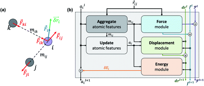 |
| | Fig. 1 (a) Newton's laws for the force and displacement calculations for atom i with respect to its neighbors. (b) Schematic view of the NewtonNet message passing layer. At each layer four separate components are updated: atomic feature arrays ai, latent force vectors  and force and displacement feature vectors (f and dr). and force and displacement feature vectors (f and dr). | |
Atomic feature aggregator
We initialize the atomic features based on trainable embedding of atomic numbers Zi, i.e., a0i = g(Zi) and  We next use the edge function
  to represent the interatomic distances using radial Bessel functions as introduced by Klicpera et al.9
| | 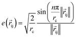 | (4) |
where rc is the cutoff radius and  returns the interatomic distance between any atom i and j. We follow Schutt et al.16 in using a self-interaction linear layer
  to combine the output of radial basis functions with each other. This operation is followed by using an envelop function to implement a continuous radial cutoff around each atom. For this purpose, we use the polynomial function ecut introduced by Klicpera et al.9 with the choice of degree of polynomial p = 7. Thus, the edge operation
  is defined as a trainable transformation of relative atom position vectors in the cutoff radius rc
| | 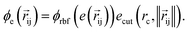 | (5) |
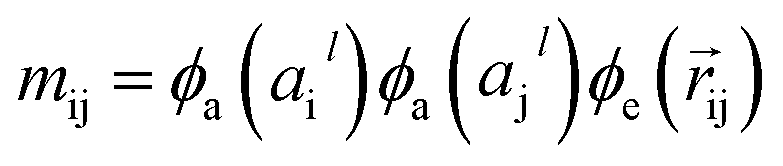
The output of ϕe is rotationally invariant as it only depends on the interatomic distances. Following the notation of neural message passing, we define a message function to collect the neighboring information and update atomic features. Here, we tend to pass a symmetric message between any pair of atoms, i.e., the message that is passed between atom i and atom j are the same in both directions. Thus, we introduce our symmetric message passing mij by element-wise product between all feature arrays involved in any two-body interaction,| | 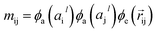 | (6) |
where  indicates a trainable and differentiable network with a nonlinear activation function SiLU19 after the first layer. Note that the ϕa is the same function applied to all atoms. Thus, due to the weight sharing and multiplication of output features of both heads of the two-body interaction, the mij remain symmetric at each layer of message passing. To complete the feature array aggregator, we use the eqn (2) to simply sum all messages received by central atom i from its neighbors
  Finally, we update the atomic features at each layer using the sum of received messages,
| |  | (7) |
Force calculator
So far, we have followed a standard message passing that is invariant to the rotation. We begin to take advantage of directional information starting from the force calculator module. The core idea behind this module is to construct latent force vectors using the Newton's third law. The third law states that the force that atom i exerts on atom j is equal and in opposite direction of the force that atom j exerts on atom i. This is the reason that we intended to introduce a symmetric message passing operator. Thus, we can estimate the symmetric force magnitude as a function of mij, i.e.,  The product of the force magnitude by unit distance vectors
  gives us antisymmetric interatomic forces that obey the Newton's third law (note that
  ),
),| |  | (8) |
where  is a differentiable learned function, and
  The total force at each layer
  on atom i is the sum of all the forces from the neighboring atoms j in the atomic environment,
| |  | (9) |
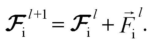
and updating the latent force vectors at each layer,| | 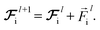 | (10) |
We ultimately use the latent force vector from the last layer L,  in the loss function to ensure this latent space truly mimics the underlying physical rules.
To complete the force calculator module, we borrow the idea of continuous filter from Schut et al. to decompose and scale latent force vectors along each dimension using another learned function  This way we can featurize the vector field to avoid too much of abstraction in the structural information that they carry with themselves,
| | 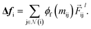 | (11) |
As a result, the constructed latent interatomic forces are decomposed by rotationally invariant features along each dimension,
i.e.,

We call this type of representation feature vectors. Following the message passing strategy, we update the force feature vectors with
Δfi after each layer, while they are initialized with zero values,
f0i = 0,
Momentum calculator
This is the step that we try to estimate a measure of atomic displacement due to the forces that are exerted on them. We accumulate their displacements at each layer without updating the position of each atom. The main idea in this module is that the displacement must be along the updated force features in the previous step. Inspired by Newton's second law, we approximate the displacement factor using a learned function  that acts on the current state of each atom presented by its atomic features ail,
| | | δri = ϕr(ail+1)fil+1. | (13) |
We finally update the displacement feature vectors by δri and a weighted sum of all the atomic displacements from the previous layer. The weights are estimated based on a trainable function of messages 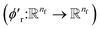 between atoms,
| | 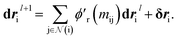 | (14) |
The weight component in this step works like attention mechanism to concentrate on the two-body interactions that cause maximum movement in the atoms. Since forces at l = 0 are zero, the displacements are also initialized with zero values, i.e., dr0i = 0.
Energy calculator
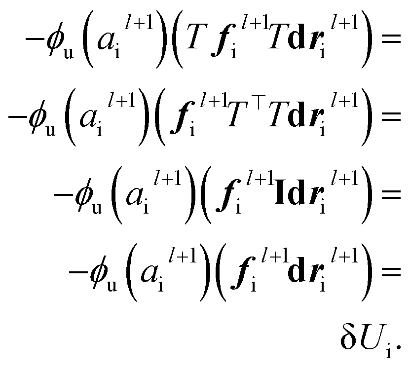
The last module contracts the directional information to the rotationally invariant atomic features. Since we developed the previous steps based on the Newton's equations of motion, one immediate idea is to approximate the potential energy change for each atom using fil and δril, resembling fil ≈ −δU/δril in the higher dimensional space  Thus, we find energy change for each atom by
| | | δUi = −ϕu(ail+1)〈fil+1dril+1〉, | (15) |
where  and
and  is a differentiable learned function that operates on the atomic features and predicts the energy coefficient for each atom. The dot product of two feature vectors contracts the features along each dimension to a single feature array. We finally update the atomic features once again using the contracted directional information presented as atomic potential energy change,This approach is both physically and mathematically consistent with the rotational equivariance operations and the goals of our model development. Physically, the energy change is the meaningful addition to the atomic feature arrays as they are used to predict the atomic energies eventually. Mathematically, the dot product of two feature vectors contracts the rotationally equivariant features to invariant features similar to euclidean distance that we used in the atomic feature aggregator module. Note that none of the force, displacement or energy modules are directly mapped to the final energy and force predictions. These are intermediate steps that update atomic features iteratively beyond the immediate neighborhood of each atom.
Results
Here we show that the NewtonNet model is capable of predicting the energies and forces across a wide range of available chemical data sets, thereby covering much of the application space for which machine learning models are being developed and used by other research groups.
Single small molecules
We first evaluate the performance of NewtonNet on the data generated from molecular dynamics trajectories using Density Functional Theory (DFT)20 for 9 small organic molecules from the MD17 (ref. 21 and 22) and the revised MD17 (ref. 23) benchmarks. Despite reported outliers in the calculated energies associated with the original version of the MD17 data, we still show it for completeness. For training NewtonNet, we select a data size of 950 for training, 50 for validation, and remaining data for test (more than 100k per molecule); this data split is more ambitious than that used by kernel methods such as sGDML24 and FCHL19,23 and is supported by other emerging machine learning models that utilize equivariant operators, e.g., NequIP13 and PaiNN.16Table 1 and ESI Table 1† shows the performance of NewtonNet for both energy and forces on the hold-out test set for both MD17 data sets, illustrating that it can outperform invariant deep learning models (e.g., SchNet,7 PhysNet,8 and DimeNet9) and even in some cases state-of-the-art equivariant models such as NequIP (using the original rank 1 version) and PaiNN.
Table 1 The performance of models in terms of mean absolute error (MAE) for the prediction of energies (kcal mol−1) and forces (kcal mol−1 Å−1) of molecules in the MD17 data sets. We report results by averaging over four random splits of the data to define standard deviations. Best results in the standard deviation range are marked in bold
|
|
|
SchNet |
PhysNet |
DimeNet |
FCHL19 |
sGDML |
NequIP (l = 1) |
PaiNN |
NewtonNet |
|
Aspirin
|
Energy |
0.370 |
0.230 |
0.204 |
0.182 |
0.19 |
— |
0.159
|
0.168 ± 0.019 |
| Forces |
1.35 |
0.605 |
0.499 |
0.478 |
0.68 |
0.348
|
0.371 |
0.348 ± 0.014 |
| Ethanol |
Energy |
0.08 |
0.059 |
0.064 |
0.054
|
0.07 |
— |
0.063 |
0.078 ± 0.010 |
| Forces |
0.39 |
0.160 |
0.230 |
0.136
|
0.33 |
0.208 |
0.230 |
0.264 ± 0.032 |
| Malonaldehyde |
Energy |
0.13 |
0.094 |
0.104 |
0.081
|
0.10 |
— |
0.091 |
0.096 ± 0.013 |
| Forces |
0.66 |
0.319 |
0.383 |
0.245
|
0.41 |
0.337 |
0.319 |
0.323 ± 0.019 |
|
Naphthalene
|
Energy |
0.16 |
0.142 |
0.122 |
0.117
|
0.12 |
— |
0.117
|
0.118 ± 0.002 |
| Forces |
0.58 |
0.310 |
0.215 |
0.151 |
0.11 |
0.096 |
0.083
|
0.084 ± 0.006 |
|
Salicylic acid
|
Energy |
0.20 |
0.126 |
0.134 |
0.114 |
0.12 |
— |
0.114
|
0.115 ± 0.008 |
| Forces |
0.85 |
0.337 |
0.374 |
0.221 |
0.28 |
0.238 |
0.209 |
0.197 ± 0.004 |
|
Toluene
|
Energy |
0.12 |
0.100 |
0.102 |
0.098
|
0.10 |
— |
0.097
|
0.094 ± 0.005 |
| Forces |
0.57 |
0.191 |
0.216 |
0.203 |
0.14 |
0.101 |
0.102 |
0.088 ± 0.002 |
| Uracil |
Energy |
0.14 |
0.108 |
0.115 |
0.104
|
0.11 |
— |
0.104
|
0.107 ± 0.004 |
| Forces |
0.56 |
0.218 |
0.301 |
0.105
|
0.24 |
0.172 |
0.140 |
0.149 ± 0.003 |
|
Azobenzene
|
Energy |
— |
0.197 |
— |
— |
0.092
|
— |
— |
0.142 ± 0.003 |
| Forces |
— |
0.462 |
— |
— |
0.409 |
— |
— |
0.138 ± 0.010 |
|
Paracetamol
|
Energy |
— |
0.181 |
— |
— |
0.153 |
— |
— |
0.135 ± 0.004 |
| Forces |
— |
0.519 |
— |
— |
0.491 |
— |
— |
0.263 ± 0.010 |
On a similar task we train NewtonNet on the CCSD/CCSD(T) data reported for 5 small molecules.21,22 The significance of this experiment is the gold standard of theory that is used to obtain the data, and addressing the ultimate goal to evaluate a machine learning model at high reference accuracy with an affordable number of training samples. In this benchmark data, the training and test splits are fixed at that provided by the authors of the MD17 data (i.e., 1000 training and 500 test data).22 In Table 2 we compare our results with NequIP and sGDML in which NewtonNet not only outperforms the best reported prediction performance for three of the five molecules, but it remains competitive within the range of uncertainties for the other two molecules, and is robustly improved compared to the opponent kernel methods. More recently NequIP has updated their results by considering higher tensor ranks (l > 1) and addition of translation equivariant features in the same preprint reference. We consider these additions very promising if the computational cost of more complex operators are justified. A benefit of NewtonNet is that it is computationally efficient and scalable relative to the newer equivariant methods that incorporate higher order tensors in the equivariant operators,13,14 while still retaining chemical accuracy (<0.5 kcal mol−1).
Table 2 The performance of models in terms of mean absolute error (MAE) for the prediction of energies (kcal mol−1) and forces (kcal mol−1 Å−1) of molecules at CCSD or CCSD(T) accuracy. We randomly select 50 snapshots of the training data as the validation set and average the performance of NewtonNet over four random splits to find standard deviations. Best results in the standard deviation range are marked in bold
|
|
|
sGDML |
NequIP (l = 1) |
NewtonNet |
| Aspirin |
Energy |
0.158 |
— |
0.100 ± 0.007 |
| Forces |
0.761 |
0.339
|
0.356 ± 0.019 |
| Benzene |
Energy |
0.003
|
— |
0.004 ± 0.001 |
| Forces |
0.039 |
0.018 |
0.011 ± 0.001 |
| Ethanol |
Energy |
0.050
|
— |
0.049 ± 0.007 |
| Forces |
0.350 |
0.217
|
0.282 ± 0.032 |
| Malonaldehyde |
Energy |
0.248 |
— |
0.045 ± 0.004 |
| Forces |
0.369 |
0.369 |
0.285 ± 0.038 |
| Toluene |
Energy |
0.030 |
— |
0.014 ± 0.001 |
| Forces |
0.210 |
0.101 |
0.080 ± 0.005 |
Small molecules with large chemical variations
In a separate experiment to validate NewtonNet we trained it using the ANI-1 dataset to predict energies for a large and diverse set of 20 million conformations sampled from ∼ 58k small molecules with up to 8 heavy atoms.25 The challenges in regards to this dataset are three-fold: first, the molecular compositions and conformations are quite diverse, with the total number of atoms ranging from 2 to 26, and with total energies spanning a range of near 3 × 10⁵ kcal mol−1; second, only energy information is provided, so a well-trained network needs to extract information more efficiently from the dataset to outcompete data-intensive invariant models; finally, a machine learning model that performs well on such a diverse dataset is more transferable to unseen data, and will have a wider application domain.
We tested the performance of NewtonNet on the ANI-1 dataset following the protocol described in ref. 20, using 80% of the conformations from each molecule for training, 10% for validation and 10% for testing. In Table 3 we show that by utilizing only 10% (2 M) samples of the original ANI-1 data, NewtonNet yields a MAE in energies of 0.65 kcal mol−1, very near the standard definitions of chemical accuracy, and halving the error compared to ANNs using the full 20 M ANI-1 dataset. Even with only 5% of the data (1 M), we achieve an MAE of 0.85 kcal mol−1 on energies that exceeds the original performance of the ANN network trained with all data. Note that unlike the data experiments above, atomic forces are not reported with the ANI-1 data set. Although the NewtonNet model is trained without taking advantage of additional force information for the atomic environments, it clearly confirms that the directional information are generally a significant completion to the atomic feature representation regardless of the tensor order of the output properties.
Table 3 The test performance of the NewtonNet model on small fractions of the original 20 million molecules ANI-1.25 We also consider data sets derived from active learning including the ANI-1X26 and alkane pyrolysis27 data sets. The 3 data sets are reported in terms of mean absolute error (MAE) for energies (kcal mol−1) and forces (kcal mol−1 Å−1). The ANI-1X energy and force errors are reported as the performance of the NewtonNet model on the COMP6 benchmark only considering conformations of a given molecule within 100 kcal mol−1 energy range to compare with those reported by Smith et al.26 For the 10% training of the ANI-1X data, we randomly sampled 5000 frames from the remaining and complete ANI-1X data for test set. For the alkane pyrolysis dataset, we randomly sampled 7100 frames from the 35![[thin space (1/6-em)]](https://www.rsc.org/images/entities/char_2009.gif) 496 training frames to define the test set
496 training frames to define the test set
| training set size |
ANI |
NewtonNet |
NewtonNet |
| 20,000000 |
2000000 |
1000000 |
|
The test set performance for the alkane pyrolysis reaction was not reported in ref. 22, so we compared our test set performance with the training set performance in ref. 22.
|
| Energies |
1.30 |
0.65 |
0.85 |
| training set size |
ANI-1X |
NewtonNet |
| 4956005 |
495600 |
| Energies |
1.61 |
1.45 |
| Forces |
2.70 |
1.79 |
| training set size |
Alkane pyrolysisa |
NewtonNet |
NewtonNet |
| 35496 |
28396 |
10000 |
| Forces (train) |
9.68 |
5.69 |
7.58 |
| Forces (test) |
— |
6.50 |
8.71 |
Reducing required data on active learning datasets
An active learning (AL) approach has been suggested as a means to further improve ANN performance through better data sampling, reducing data requirements to 10–25% of the original ANI data set as reported by Smith and coworkers.26 We have tested NewtonNet on two datasets generated through an AL approach, and in Table 3 we show that we can make improved predictions on the active learning extended ANI-1X data set reported by Smith and co-worker26 as well as active learning data generated for linear alkane pyrolysis.27 For the ANI-1X dataset, we achieve better energy and force predictions on the test set with as low as 10% of all training data that was created through an active learning procedure. For the alkane pyrolysis dataset, we are able to achieve better force predictions on the test set when compared to the mean absolute error of forces on the training set of the original work, by utilizing as low as 30% of all training data.
The better performance of NewtonNet on these two datasets suggests that our model is capable of utilizing information more efficiently, even from dataset with limited sizes and concentrated information such as those created by AL. However in both cases the original AI models lack equivariant features, and as this will propagate into the AL sampling approach, it is therefore not a complete proof of optimality for NewtonNet. Instead training NewtonNet using an AL sampling approach would be required to fully take advantage of the improved ML model capabilities in addition to biasing the distribution of training date towards more difficult examples. In future work we hope to test whether further performance enhancements beyond that reported in Table 3 is realized once NewtonNet is combined with AL training.
Methane combustion reaction
The methane combustion reaction data28 exerts a more challenging task due to the complex nature of reactive species that are often high in energy, transient, and far from equilibrium such as free radical intermediates. Such stress tests are important for driving ab initio molecular dynamics simulations in which even relatively low-run DFT functionals are notoriously time-consuming and limited to small system sizes. We utilized the dataset provided by Zeng et al.,28 which contains 578731 snapshots for training. We trained NewtonNet on 100%, 10% and 1% of the data and evaluated the performance of NewtonNet on two hold-out test sets. One test set is provided by the original authors, comprised of 13315 snapshots generated using the same procedure as the training data and we refer to it as out-of-distribution (OOD) hold-out test set. The other set is 13315 random samples of training data that we hold out as the final test set and we refer to it as in-distribution (ID) hold-out test set. The main reason for considering two test sets is the large energy and force distribution shifts that is found between the original training and test sets.
The prediction correlation plots for both energies and forces on the ID test set and OOD test set of NewtonNet trained with 100% data were provided in ESI Fig. 1.†Table 4 shows that when NewtonNet is trained on all available data, it drives down the ID test error in energies and forces significantly, even outperforming the reported training error of the original DeepMD model.28 Even when utilizing as low as 1% of the training data, NewtonNet still has an MAE on the ID hold-out test set that is close to chemical accuracy on energy prediction. Even though a distribution shift was observed between the original train and test sets, NewtonNet still has competitive energy and force prediction accuracy on the out-of-distribution test dataset. Given the similar performance of NewtonNet on OOD test set with 100% and 10% of training data, we argue the comparison on the OOD test set is mainly influenced by the aforementioned distribution shift.
Table 4 The performance of NewtonNet model compared with DeepMD on 13315 randomly sampled in-distribution (ID) hold-out test configurations and 13315 out-of-distribution (OOD) test configurations provided by the authors on the methane combustion dataset. Errors are reported in terms of mean absolute error (MAE) for energies (kcal per mol per atom) and forces (kcal mol−1 Å−1). We systematically reduce the amount of training data by two orders of magnitude using NewtonNet and compare it to the 578731 data points used in the original paper by Zeng and co-workers28
| Training set size |
DeepMD |
NewtonNet |
NewtonNet |
NewtonNet |
| 578731 |
578731 |
57873 |
5787 |
|
The MAE on the training set reported in ref. 14 was taken as the in-distribution prediction error here.
|
| Energies (ID) |
0.945a |
0.353 |
0.391 |
0.484 |
| Forces (ID) |
— |
1.12 |
1.88 |
2.78 |
| Energies (OOD) |
3.227 |
3.170 |
3.135 |
3.273 |
| Forces (OOD) |
2.77 |
2.75 |
2.93 |
3.76 |
Hydrogen combustion reaction
This benchmark data is newly generated for this study and probes reactive pathways of hydrogen and oxygen atoms through the combustion reaction mechanism reported by Li et al.,29 and analyzed with calculated intrinsic reaction coordinate (IRC) scans of 19 biomolecular sub-reactions from Bertels et al.30 Excluding 3 reactions that are chemically trivial (diatomic dissociation or recombination reactions), we obtain configurations and energies and forces for reactant, transition, and product states for 16 out of 19 reactions. The IRC data set was further augmented with normal mode displacements and AIMD simulations to sample configurations around the reaction path. All the calculations are conducted at the ωB97M-V/cc-pVTZ level of theory, and the data set comprises a total of ∼280000 potential energies and ∼1240000 nuclear force vectors, and will be described in an upcoming publication.
We train NewtonNet on the complete reaction network by sampling training, validation, and test sets randomly formulated from the total data. The validation and test sizes are fixed to 1000 data per reaction, and the size of training data varies in a range of 100 to 5000 data points per reaction. The resulting model accuracy on the hold-out test set for both energy and forces is reported in Fig. 2. It is seen that NewtonNet can outperform the best invariant SchNet model with slightly more than one order of magnitude smaller training data (500 vs. 5000 samples per reaction), and is capable of achieving the chemical accuracy goal with as little as 500 data points per reaction. We integrate this model with the ASE interface31 to run MD. A sample run is provided in ESI Fig. 2† to demonstrate energy conservation. A more thorough study on this system using NewtonNet will come in later publications. In conventional deep learning approaches for reactive chemistry, abrupt changes in the force magnitudes can give rise to multimodal distributions of data, which can introduce covariate shift in the training of the models. Here we posit that a better representation of atomic environments using the latent force directions can increase the amount of attention that one atom gives to its immediate neighbors. As a result the performance of NewtonNet in prediction of forces for methane and hydrogen combustion reactive systems benefit most from the directional information provided by atoms that break or form new bonds.
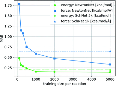 |
| | Fig. 2 The learning curve of NewtonNet for the hydrogen combustion data, with MAEs of energy and forces averaged over the 16 independent reactions and with respect to the number of training samples used for each reaction. The dashed lines show the performance of SchNet when trained on all 5k data per sub-reaction. | |
Discussion
Ablation study
We justify our design choices for the NewtonNet architecture with ablation of network components on the example of the aspirin MD trajectory from the MD17 data set. Compared to the original design, we break the symmetric message passing in eqn (6) by removing self atomic feature multiplication, and we investigate zeroing out the weight of latent force reconstruction loss in which the latent force vectors are not guided to the atomic forces direction. Note that in all these changes the number of model parameters remains constant.
Table 5 shows the results for various combination of these ablated components. The performance of the model deteriorates after each ablation, with the maximum change for breaking the symmetry and minimum change for removing the latent force reconstruction loss. The ablation of both together is also tested to confirm that even without the latent force loss, the entire design still needs to follow Newtonian rules (e.g., via the ablated symmetric message passing) to achieve its best performance. Based on our hyperparameter search, we have noticed that the weight of different loss components can significantly change the focus of the model on the energy or force optimization. We generally recommend a higher weight for force loss (λF) compared to other components. The weight of latent force loss (λD) can be even removed or faded out for some chemical systems with no or minimum change in the overall performance. However, breaking the second Newton law in our symmetric message passing function worsens the prediction performance significantly.
Table 5 Ablation study with a focus on the Newtonian components of our model. Numbers show the MAE of energy (kcal mol−1) and force (kcal mol−1 Å−1) predictions for aspirin molecule from MD17
|
|
Energy |
Forces |
| No ablation |
0.168 ± 0.019 |
0.348 ± 0.014 |
| Remove sym. message passing |
4.430 ± 2.020 |
4.290 ± 0.360 |
| Remove latent force loss |
0.167 ± 0.014 |
0.359 ± 0.013 |
| Remove both |
0.187 ± 0.022 |
0.427 ± 0.009 |
Computational efficiency of NewtonNet
In addition to data efficiency as illustrated in Results, NewtonNet allows for a linear scaling in computational complexity with respect to the number of atoms in the system. This can be mathematically proven since the value of all operators are proportional to the size of the system with the assumption that all neighbors are in a small cutoff radius. To give a better sense of the computational efficiency we compare the time that is needed to train on the aspirin molecule from the MD17 data set with the same calculation using the NequIP model. As reported by Batzner et al., a complete training on the MD17 data to converge to the best performance of NequIP model takes up to 8 days.13 However, NewtonNet only required 12 hours to give the state-of-the-art performance on a GeForce RTX 2080Ti, GPU which is only 73% as fast as the Tesla V100 that is used for evaluating NequIP, when a straightforward comparison of similar rank of contributed tensors used by both methods. Obviously, higher order tensors may boost performance but will increase the computation time, and should be analyzed from a cost-benefit perspective to find the best level of ML models for the required accuracy versus computational resources.
Aside from training time that is important to facilitate the model development and to reduce the testing time, the computation time per atomic environment is critical for the future application of trained models in an MD simulation. The computation time for processing a snapshot of the MD trajectory of a small molecule by NewtonNet is 4 milliseconds (∼3 ms on a Tesla V100) for a small molecule of 20 atoms. Considering the reported average time of 16 milliseconds for NequIP to process a molecule of 15 atoms,13 NewtonNet demonstrates a significant speedup. In addition, the PaiNN model16 is the closest to our model in terms of computational complexity, but does not encode additional physical knowledge in the message passing operators. As a result, it includes about 20% more number of optimized parameters (600k vs. 500k parameters in NewtonNet). This difference likely leads to higher computational cost with an equally efficient implementation of the code. Nevertheless, all these reported prediction times are by far smaller than ab initio calculations even for a snapshot of a small molecule in the MD trajectory, which is on the order of minutes to hours.
Conclusions
The ability to predict the energy and forces of a molecular dynamics trajectory with high accuracy but at an efficient time scale is of considerable importance in the study of chemical and biochemical systems. We have developed a new ML model based on Newton's equation of motion that can conduct this task more accurately (or achieve competitive performance) than other state-of-the-art invariant and equivariant models.
Overall, the presented results are promising in at least three major respects. First, since the NewtonNet model takes advantage of geometric message passing and a rotationally equivariant latent space which scales linearly with the size of the system, its promising performance in accuracy can be achieved without much computation or memory overhead. NewtonNet, like other equivariant deep learning models, utilizes less data and can still outperform the kernel methods that are renowned for their good performance on small size data. Given the better scalability of deep learning models such as NewtonNet compared to kernel methods, we can expand the training data, for example by smart sampling methods like active learning32,33 and explore the potential energy surface of the chemical compound space more efficiently. The study of methane combustion reaction is a proof of evidence for this approach as the training data is a result of active learning sampling. If this sampling was initiated with NewtonNet predictions, one could achieve the best performance with even less number of queries.
Second, the data efficiency is the key to achieve ML force field models at the high accuracy levels of first principles methods such as CCSD(T)/CBS with competitive performances as state-of-the-art kernel-based methods using significantly less training data. For the CCSD(T) data on small single organic molecules we found that the NewtonNet performance is competitive or better than state-of-the-art equivariant models by at least 10%. This is a very encouraging result for being able to obtain gold standard levels of theory with affordable data set generation.
Finally, taking advantage of Newton's laws of motion in the design of the architecture helped to avoid unnecessary operations, and provide a more understandable and interpretable latent space to carry out the final predictions. Inspired by other physical operations that incorporate higher order tensors,13,14 NewtonNet can also be further extended to construct more distinguishable latent space many-body features in future work. Even so, the performance of the NewtonNet model on the MD trajectories from combustion reactions are both excellent with good chemical accuracy even when considering the challenge of chemical reactivity.
The idea to utilize directional information in neural networks in the form of equivariant operators is so recent that their broader application in chemical sciences are still in their early stage. One key feature in our experiments is the existence of atomic labels (i.e., forces) that help to propagate directional information smoothly and robustly. When outputs are only provided in a more abstract way (e.g., predicting molecular properties), the addition of domain knowledge in the form of regularizers or normalization layers34 remain a challenge that domain researchers need to overcome to achieve the state of the art performance.
Appendix A. Proof of equivariance and invariance
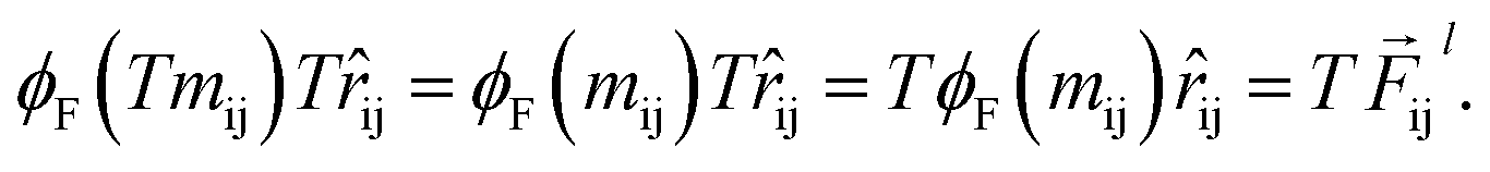
We prove that our model is rotationally equivariant on the atomic positions  and atomic numbers Zi for a rotation matrix
  In eqn (1), the euclidean distance is invariant to the rotation, as it can be shown that
| | 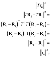 | (17) |
Which means that the euclidean distance is indifferent to the rotation of the positions as it is quite well-known for this feature. Consequently, feature arrays mij, ai, and all the linear or non-linear functions acting on them will result in invariant outputs. The only assumptions for this proof is that a linear combination of vectors or their product with invariant features will remain rotationally equivariant. Base on this assumption we claim that eqn (5)–(11) will remain equivariant to the rotations. For instance, the same rotation matrix T propagates to eqn (5) such that,
| |  | (18) |
The last operator, eqn (12), will remain invariant to the rotations due to the use of dot product. The proof for the invariant atomic energy changes is that,
| |  | (19) |
This is how we contract equivariant features to invariant arrays. The addition of these arrays to atomic features preserves the invariance for the final prediction of atomic contributions to the total potential energy.
Methods
Training details
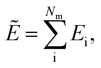
We follow the summation rule as described by Behler and Parrinello5 to predict the atomic energies. Following this rule, we use a differentiable function to map the updated atomic features after last layer aiL to atomic potential energies Ei. Ultimately, the total potential energy is predicted as the sum of all atomic energies.| |  | (21) |
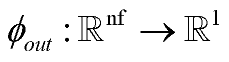
where Nm is the total number of atoms, and  is a fully connected network with Sigmoid Linear Unit (SiLU) activation19 after each layer except the last layer.
To accelerate training and achieve better generalizability, we applied two different data normalization approaches. For the dedicated small molecule models, we normalized the total potential energies Ẽ with fixed mean and standard deviation calculated from the training dataset. For methane combustion reaction models, we normalized the atomic potential energies Ei using trainable mean and standard deviation, and inverse normalize atomic energies before summing them up to allow variability in species compositions.
We obtain forces as gradient of potential energy with respect to atomic positions. This way we guarantee the energy conservation23 and provide atomic forces for a robust training of the atomic environments,
| | ![[F with combining tilde]](https://www.rsc.org/images/entities/i_char_0046_0303.gif) i = −∇iẼ. i = −∇iẼ. | (22) |
We train the model using small batches of data with batch size M. The loss function penalizes the model for predicted energy values, force components, and the direction of latent force vectors from last message passing layer  . These three terms of the loss function
  are formulated as:
| | 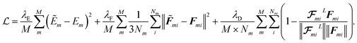 | (23) |
The first two terms are common choices for the energy and forces that are on the basis of the mean squared deviations of predicted values with references data. The last term penalizes the deviation of latent force vectors direction with the ground-truth force vectors. Here, we use cosine similarity loss function to minimize the (1 − cos(α)) ∈ [0, 2], where α is the angle between the  and Fi for each atom i of a snapshot m of a MD trajectory. The λE, λF, and λD are hyperparameters that determine the contribution of energy, force, and latent force direction losses in the total loss
We use mini-batch gradient descent algorithm (with Adam optimizer35) to minimize the loss function with respect to the trainable parameters. The trainable parameters are built in the learned functions noted with ϕ symbol. We use fully connected neural network with SiLU nonlinearity for all ϕ functions through out the message passing layer. The only exception is the ϕrbf, which is a single linear layer. We avoid using bias parameters in the ϕf and  in order to propagate the radial cutoff throughout the network. We found it important for the ANI model to use a normalization layer36 on the atomic features at every message passing layer as it helps with the stability of training. All NewtonNet models in this paper use L = 3 message passing layers, nf = 128 features and nb = 20 basis sets. The number of features are set similar to previous works to emphasize on the impact of architecture design in our comparisons. Other hyper-parameters are selected based on the best practices for each type of system and are reported in the Table 6.
Table 6 Hyperparameters for all the reported experiments in the results section
|
|
λ
E
|
λ
F
|
λ
D
|
Learning rate (lr) |
lr decay |
Cutoff radius [Å] |
|
10% data & 1% data.
100% data.
|
| MD17 |
1 |
50 |
1 |
1 × 10⁻³ |
0.7 |
5 |
| MD17/CCSD(T) |
1 |
50 |
1 |
1 × 10⁻³ |
0.7 |
5 |
| ANI |
1 |
0 |
0 |
1 × 10⁻⁴ |
0.7 |
5 |
| Methane combustiona |
1 |
5 |
1 |
1 × 10⁻³ |
0.7 |
5 |
| Methane combustionb |
1 |
5 |
1 |
1 × 10⁻⁴ |
0.7 |
5 |
| Hydrogen combustion |
1 |
20 |
1 |
5 × 10⁻⁴ |
0.7 |
5 |
For the training of SchNet in the hydrogen combustion study we use 128 features everywhere and 5 interaction layers as recommended by developers.7 The other hyperparameters are the same as NewtonNet except for the force coefficient in the loss function that we found a lower λF = 10 performs better than larger coefficients.
Data and code availability
The GitHub repository is publicly available and open source at https://github.com/THGLab/NewtonNet. We also designed a command line interface to facilitate faster implementation by non-programmers. Although the new hydrogen combustion data is currently under review it has been made available at https://github.com/THGLab/H2COMBUSTION_DATA, https://doi.org/10.6084/m9.figshare.19601689.
Author contributions
T. H-G. and M. H. conceived the scientific direction and wrote the complete manuscript. M. H., J. L., X. G., O. Z., M. L., and H. H. ran experiments with NewtonNet and other ML models on the various datasets and wrote the corresponding Results in the manuscript. A. D., C. J. S., L. B. and F. H-Z. generated the hydrogen combustion data. T. H-G., M. H., J. L., O. Z., F. H-Z., and X. G analyzed the results. All authors provided comments on the results and manuscript.
Conflicts of interest
The authors declare no competing interests.
Acknowledgements
The authors thank the National Institutes of Health for support under Grant No 5U01GM121667 for support of the machine learning method. We also thank the National Science Foundation under grant CHE-1955643 for support of the chemical application of hydrogen combustion. FHZ thanks the Research Foundation-Flanders (FWO) Postdoctoral Fellowship for support as a visiting Berkeley scholar. M. Liu thanks the China Scholarship Council for a visiting scholar fellowship. C. J. S. acknowledges funding by the Ministry of Innovation, Science and Research of North Rhine-Westphalia (“NRW Rückkehrerprogramm”) and an Early Postdoc. Mobility fellowship from the Swiss National Science Foundation. This research used computational resources of the National Energy Research Scientific Computing Center, a DOE Office of Science User Facility supported by the Office of Science of the U.S. Department of Energy under Contract No. DE-AC02-05CH11231.
References
- A. L. Ferguson and K. A. Brown, Data-driven design and autonomous experimentation in soft and biological materials engineering, Annu. Rev. Chem. Biomol. Eng., 2022, 13(1) DOI:10.1146/annurev-chembioeng-092120-020803.
- M. Garcia de Lomana, F. Svensson, A. Volkamer, M. Mathea and J. Kirchmair, Consideration of predicted small-molecule metabolites in computational toxicology, Digital Discovery, 2022, 1(2), 158–172, 10.1039/D1DD00018G.
- K. Chen, C. Kunkel, K. Reuter and J. T. Margraf, Reorganization energies of flexible organic molecules as a challenging target for machine learning enhanced virtual screening, Digital Discovery, 2022, 1(2), 147–157, 10.1039/D1DD00038A.
- D. Bash, F. Hubert Chenardy, Z. Ren, J. J. Cheng, T. Buonassisi, R. Oliveira, J. N. Kumar and K. Hippalgaonkar, Accelerated automated screening of viscous graphene suspensions with various surfactants for optimal electrical conductivity, Digital Discovery, 2022, 1(2), 139–146, 10.1039/D1DD00008J.
- J. Behler and M. Parrinello, Generalized neural-network representation of high-dimensional potential-energy surfaces, Phys. Rev. Lett., 2007, 98, 146401, DOI:10.1103/PhysRevLett.98.146401.
-
J. Gilmer, S. S. Schoenholz, P. F. Riley, O. Vinyals, and G. E. Dahl, Neural Message Passing for Quantum Chemistry, in Proc. 34th Int. Conf. Mach. Learn. – Vol. 70, ICML'17, 2017, pp. 1263–1272, https://JMLR.org Search PubMed.
- K. T. Schütt, P. Kessel, M. Gastegger, K. A. Nicoli, A. Tkatchenko and K.-R. M. Schnetpack, A deep learning toolbox for atomistic systems, J. Chem. Theory Comput., 2019, 15(1), 448–455, DOI:10.1021/acs.jctc.8b00908.
- T. Oliver, Unke and Markus Meuwly. PhysNet: A Neural Network for Predicting Energies, Forces, Dipole Moments, and Partial Charges, J. Chem. Theory Comput., 2019, 15(6), 3678–3693, DOI:10.1021/acs.jctc.9b00181.
-
J. Klicpera, J. Groß, and S. Günnemann, Directional Message Passing for Molecular Graphs, 2020, arXiv preprint arXiv:2003.03123v1, pp. 1–13.
-
R. Kondor, Z. Lin, and S. Trivedi, Clebsch–Gordan nets: a fully Fourier space spherical convolutional neural network, in Advances in Neural Information Processing Systems, ed. S. Bengio, H. Wallach, H. Larochelle, K. Grauman, N. Cesa-Bianchi, and R. Garnett, Vol. 31, Curran Associates, Inc., 2018 Search PubMed.
-
N. Thomas, T. Smidt, S. Kearnes, L. Yang, L. Li, K. Kohlhoff, and P. Riley, Tensor field networks: Rotation- and translation-equivariant neural networks for 3d point clouds, 2018, arXiv preprint arXiv:1802.08219.
- B. Anderson, H. Truong Son and R. Kondor, Cormorant: Covariant molecular neural networks, Adv. Neural Inf. Process. Syst., 2019, 32, 14537–14546 Search PubMed.
-
S. Batzner, T. E. Smidt, L. Sun, J. P. Mailoa, M. Kornbluth, N. Molinari, and B. Kozinsky, Se(3)-equivariant graph neural networks for data-efficient and accurate interatomic potentials, 2021, arXiv preprint arXiv:2101.03164.
-
Z. Qiao, A. S. Christensen, M. Welborn, F. R. Manby, A. Anandkumar, and T. F. Miller, Unite: Unitary n-body tensor equivariant network with applications to quantum chemistry, 2021, arXiv preprint arXiv:2105.14655.
- Z. L. Glick, A. Koutsoukas, D. L. Cheney and C. David Sherrill, Cartesian message passing neural networks for directional properties: Fast and transferable atomic multipoles, J. Chem. Phys., 2021, 154(22), 224103, DOI:10.1063/5.0050444.
-
K. T. Schütt, O. T. Unke, and M. Gastegger, Equivariant message passing for the prediction of tensorial properties and molecular spectra, 2021, arXiv preprint arXiv:2102.03150.
- F. Monti, D. Boscaini, J. Masci, E. Rodolà, J. Svoboda and M. M. Bronstein, Geometric deep learning on graphs and manifolds using mixture model CNNs, Proc. – 30th IEEE Conf. Comput. Vis. Pattern Recognition, CVPR 2017, 2017, 5425–5434, DOI:10.1109/CVPR.2017.576.
- O. Raghunath, Ramabhadran and Krishnan Raghavachari. Extrapolation to the gold-standard in quantum chemistry: Computationally efficient and accurate ccsd(t) energies for large molecules using an automated thermochemical hierarchy, J. Chem. Theory Comput., 2013, 9(9), 3986–3994, DOI:10.1021/ct400465q , PMID: 26592394, .
- S. Elfwing, E. Uchibe and K. Doya, Sigmoid-weighted linear units for neural network function approximation in reinforcement learning, Neural Networks, 2018, 107, 3–11, DOI:10.1016/j.neunet.2017.12.012.
-
R. G. Parr and Y. Weitao, Density-Functional Theory of Atoms and Molecules. International Series of Monographs on Chemistry. Oxford University Press, 1994. ISBN 9780195357738 Search PubMed.
- S. Chmiela, A. Tkatchenko, H. E. Sauceda, I. Poltavsky, K. T. Schütt, K.-r. Müller, I. Poltavsky and K. T. Sch, Machine learning of accurate energy-conserving molecular force fields, Sci. Adv., 2017, 3(5) DOI:10.1126/sciadv.1603015.
- S. Chmiela, H. E. Sauceda, K. Robert Müller and A. Tkatchenko, Towards exact molecular dynamics simulations with machine-learned force fields, Nat. Commun., 2018, 9(1), 3887, DOI:10.1038/s41467-018-06169-2.
- A. S. Christensen, L. A. Bratholm, F. A. Faber and O. Anatole von Lilienfeld, Fchl revisited: Faster and more accurate quantum machine learning, J. Chem. Phys., 2020, 152(4), 044107, DOI:10.1063/1.5126701.
- S. Chmiela, H. E. Sauceda, I. Poltavsky, K.-R. Müller and A. Tkatchenko, sGDML: Constructing accurate and data efficient molecular force fields using machine learning, Comput. Phys. Commun., 2019, 240, 38–45, DOI:10.1016/j.cpc.2019.02.007.
- J. S. Smith, O. Isayev and A. E. Roitberg, Ani-1: an extensible neural network potential with dft accuracy at force field computational cost, Chem. Sci., 2017, 8(4), 3192–3203 RSC.
- J. S. Smith, B. Nebgen, N. Lubbers, O. Isayev and A. E. Roitberg, Less is more: Sampling chemical space with active learning, J. Chem. Phys., 2018, 148(24), 241733, DOI:10.1063/1.5023802.
- J. Zeng, L. Zhang, H. Wang and T. Zhu, Exploring the chemical space of linear alkane pyrolysis via deep potential generator, Energy Fuels, 2021, 35(1), 762–769, DOI:10.1021/acs.energyfuels.0c03211.
- J. Zeng, L. Cao, M. Xu, T. Zhu and J. Z. H. Zhang, Complex reaction processes in combustion unraveled by neural network-based molecular dynamics simulation, Nat. Commun., 2020, 11(1), 1–9 CrossRef PubMed.
- J. Li, Z. Zhao, A. Kazakov and F. L. Dryer, An updated comprehensive kinetic model of hydrogen combustion, Int. J. Chem. Kinet., 2004, 36(10), 566–575, DOI:10.1002/kin.20026.
- L. W. Bertels, L. B. Newcomb, M. Alaghemandi, J. R. Green and M. Head-Gordon, Benchmarking the Performance of the ReaxFF Reactive Force Field on Hydrogen Combustion Systems, J. Phys. Chem. A, 2020, 124(27), 5631–5645, DOI:10.1021/acs.jpca.0c02734 , ISSN 15205215, .
- A. H. Larsen, J. J. Mortensen, J. Blomqvist, I. E. Castelli, R. Christensen, M. Dułak, J. Friis, M. N. Groves, B. Hammer, C. Hargus, E. D. Hermes, P. C. Jennings, P. B. Jensen, J. Kermode, J. R. Kitchin, E. L. Kolsbjerg, J. Kubal, K. Kaasbjerg, S. Lysgaard, J. B. Maronsson, T. Maxson, T. Olsen, L. Pastewka, A. Peterson, C. Rostgaard, J. Schiøtz, O. Schütt, M. Strange, K. S. Thygesen, T. Vegge, L. Vilhelmsen, M. Walter, Z. Zeng and K. W. Jacobsen, The atomic simulation environment—a python library for working with atoms, J. Phys.: Condens. Matter, 2017, 29(27), 273002 CrossRef PubMed , http://stacks.iop.org/0953-8984/29/i=27/a=273002.
- M. Haghighatlari, G. Vishwakarma, D. Altarawy, R. Subramanian and B. U. Kota, Aditya Sonpal, Srirangaraj Setlur, and Johannes Hachmann. Chemml: A machine learning and informatics program package for the analysis, mining, and modeling of chemical and materials data, Wiley Interdiscip. Rev. Comput. Mol. Sci., 2020, 10(4), e1458, DOI:10.1002/wcms.1458.
- A. Mae Miksch, T. Morawietz, J. Kästner, A. Urban and N. Artrith, Strategies for the Construction of Machine-Learning Potentials for Accurate and Efficient Atomic-Scale Simulations, Mach. Learn. Sci. Technol., 2021, 2(3), 031001, DOI:10.1088/2632-2153/abfd96.
- M. Haghighatlari, G. Vishwakarma, M. Atif Faiz Afzal and J. Hachmann, A Physics-Infused Deep Learning Model for the Prediction of Refractive Indices and Its Use for the Large-Scale Screening of Organic Compound Space, ChemRxiv, 2019, 1–9 Search PubMed.
-
P. Diederik, Kingma and Jimmy Lei Ba. Adam: A method for stochastic optimization, 3rd Int. Conf. Learn. Represent. ICLR 2015 – Conf. Track Proc., arXiv:1412.6980, 2015, pp. 1–15 Search PubMed.
-
J. Lei Ba, J. Ryan Kiros, and G. E. Hinton, 2015, Layer norm, arXiv preprint arXiv:1607.06450v1.
|
| This journal is © The Royal Society of Chemistry 2022 |
Click here to see how this site uses Cookies. View our privacy policy here. 
 Open Access Article
 This Open Access Article is licensed under a Creative Commons Attribution-Non Commercial 3.0 Unported Licence
 a,
Xingyi
Guan
ae,
Oufan
Zhang
a,
Akshaya
Das
a,
Christopher J.
Stein
a,
Xingyi
Guan
ae,
Oufan
Zhang
a,
Akshaya
Das
a,
Christopher J.
Stein
 with atomic features
  (where nf is the number of features) and interatomic attributes
  a message passing layer can be defined as:6
 and relative position vectors
  as input and applying operations that are inspired by Newton's equations of motion to create features arrays
  that represent each atom in its immediate environment with edges defined by force and displacement vectors, f and dr, respectively (Fig. 1a). NewtonNet takes advantage of multiple layers of message passing which are rotationally equivariant, described in detail below, in which each layer consists of multiple modules that include operators to construct force and displacement feature vectors, which are contracted to the feature arrays via the energy calculator module (Fig. 1b). We emphasize the critical role of projecting equivariant feature vectors to invariant arrays since one goal of the model is to predict potential energies, which are invariant to the rotations of atomic configurations. We provide the proof of equivariance of the NewtonNet model in the ESI† as well.
 and force and displacement feature vectors (f and dr).
 We next use the edge function
  to represent the interatomic distances using radial Bessel functions as introduced by Klicpera et al.9
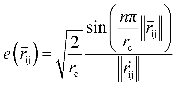
 returns the interatomic distance between any atom i and j. We follow Schutt et al.16 in using a self-interaction linear layer
  to combine the output of radial basis functions with each other. This operation is followed by using an envelop function to implement a continuous radial cutoff around each atom. For this purpose, we use the polynomial function ecut introduced by Klicpera et al.9 with the choice of degree of polynomial p = 7. Thus, the edge operation
  is defined as a trainable transformation of relative atom position vectors in the cutoff radius rc
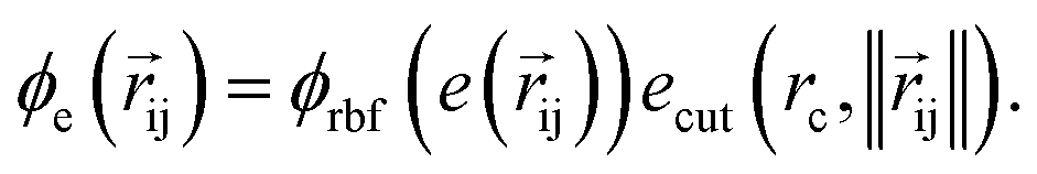
 indicates a trainable and differentiable network with a nonlinear activation function SiLU19 after the first layer. Note that the ϕa is the same function applied to all atoms. Thus, due to the weight sharing and multiplication of output features of both heads of the two-body interaction, the mij remain symmetric at each layer of message passing. To complete the feature array aggregator, we use the eqn (2) to simply sum all messages received by central atom i from its neighbors
  Finally, we update the atomic features at each layer using the sum of received messages,
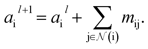
 The product of the force magnitude by unit distance vectors
  gives us antisymmetric interatomic forces that obey the Newton's third law (note that
  ),
),
 is a differentiable learned function, and
  The total force at each layer
  on atom i is the sum of all the forces from the neighboring atoms j in the atomic environment,
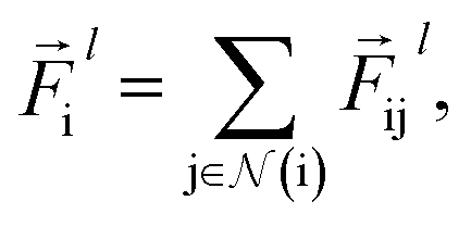
 in the loss function to ensure this latent space truly mimics the underlying physical rules.
 This way we can featurize the vector field to avoid too much of abstraction in the structural information that they carry with themselves,
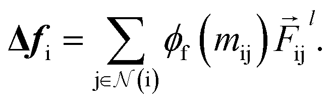
 We call this type of representation feature vectors. Following the message passing strategy, we update the force feature vectors with Δfi after each layer, while they are initialized with zero values, f0i = 0,
 that acts on the current state of each atom presented by its atomic features ail,
 between atoms,
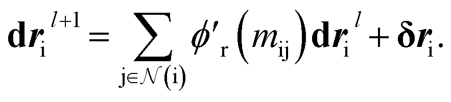
 Thus, we find energy change for each atom by
 and
and  is a differentiable learned function that operates on the atomic features and predicts the energy coefficient for each atom. The dot product of two feature vectors contracts the features along each dimension to a single feature array. We finally update the atomic features once again using the contracted directional information presented as atomic potential energy change,
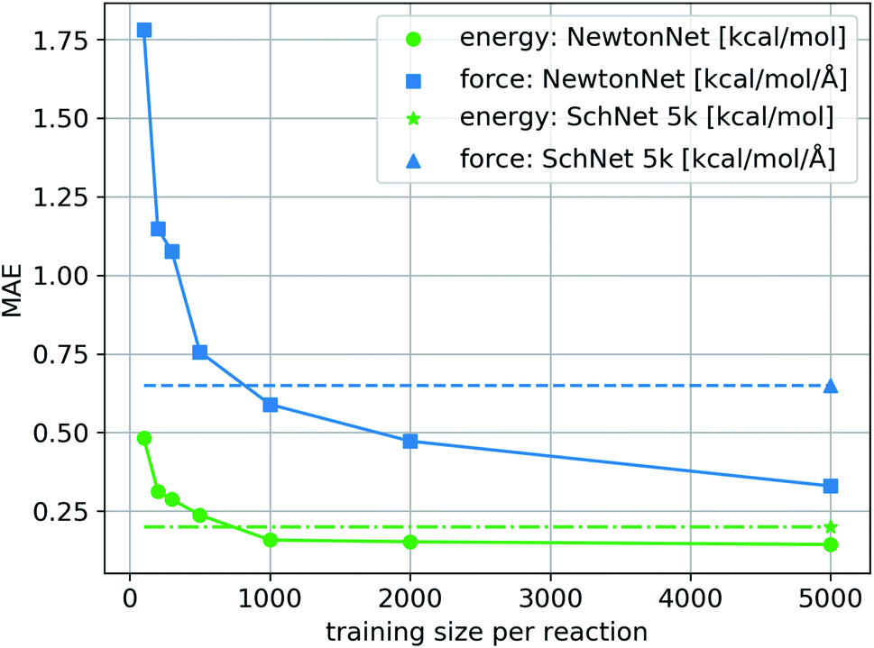
 and atomic numbers Zi for a rotation matrix
  In eqn (1), the euclidean distance is invariant to the rotation, as it can be shown that
 is a fully connected network with Sigmoid Linear Unit (SiLU) activation19 after each layer except the last layer.
 . These three terms of the loss function
  are formulated as:
 and Fi for each atom i of a snapshot m of a MD trajectory. The λE, λF, and λD are hyperparameters that determine the contribution of energy, force, and latent force direction losses in the total loss
 in order to propagate the radial cutoff throughout the network. We found it important for the ANI model to use a normalization layer36 on the atomic features at every message passing layer as it helps with the stability of training. All NewtonNet models in this paper use L = 3 message passing layers, nf = 128 features and nb = 20 basis sets. The number of features are set similar to previous works to emphasize on the impact of architecture design in our comparisons. Other hyper-parameters are selected based on the best practices for each type of system and are reported in the Table 6.